Enhancement of performance of wave turbine during stall using passive flow control : first and second law analysis

1

Enhancement of performance of Wave Turbine during Stall Using

Passive Flow Control: First and Second Law Analysis

Ahmed S. Shehata1, 2*_{, Qing Xiao} 1_{, Mohamed M. Selim}2_{, A. H. Elbatran}2_{, Day Alexander} 1

3 4

1) Department of Naval Architecture, Ocean and Marine Engineering, University of Strathclyde,

5

Glasgow G4 0LZ, U.K

6

2) College of Engineering and Technology, Arab Academy for Science Technology and Maritime

7

Transport, P.O. 1029 AbuQir, Alexandria, EGYPT

8

* Corresponding Author: Ahmed S. Shehata,

9

E-mail address: [email protected] 10

ABSTRACT

11

Wells turbine is the most common type of self-rectifying air turbine employed by Oscillating 12

Water Column (OWC) wave energy devices due to its technical simplicity, reliability, and design 13

robustness. Because it subjected to early stall, there were many endeavors to improve the energy 14

extraction performance of Wells turbine within the stall regime. Using the multi suction slots as a 15

passive flow control can help obtaining a delayed stall. Two, three and four suction slots were 16

investigated to improve the performance of Wells turbine in the stall regime. In addition the 17

commonly used first law analysis, the present study utilized an entropy generation minimization 18

method to examine the impact of the multi suction slots method on the entropy generation 19

characteristics around the turbine blade. The turbine blade with optimum suction slots number and 20

location was investigated using the oscillating water system based on the real data from the site. 21

To achieve this purpose, two-dimension numerical models for Wells turbine airfoils under 22

sinusoidal wave flow conditions were built and analyze using (ANSYS FLUENT) solver. It is 23

found that the airfoil with three suction slots located at 40%, 55% and 90% from leading edge in 24

chord percentage give the highest torque coefficient by 26.7% before the stall and 51% after the 25

stall. 26

Keywords: Oscillating flow; Wells turbine; Flow control method; Entropy generation; Egyptian 27

Coasts. 28

2

Nomenclature

1

A Total blade area (m2₎

c Blade chord (m)

𝐶𝐷 Drag force coefficient

𝐶𝐿 Lift force coefficient

𝐶_𝑇 Torque coefficient

D The fluid domain

𝐷𝑠𝑠 Suction slot diameter (m)

f cycle frequency (Hz)

D

F In-line force acting on cylinder per unit length (gf)

G The filter function

KE Kinetic Energy (W/K)

𝐿_𝑠𝑠 Suction slot location from leading edge in chord percentage %

𝐿𝑅𝑠𝑠 Reference suction slot location from leading edge in chord percentage %

K Turbulent kinetic energy

Δp Pressure difference across the turbine (N/m2₎

𝑃𝑠𝑠 Suction slot pitch distance on x axis

Δ𝑃_𝑠𝑠 Minimum distance between any two suction slot on x axis

𝑅_𝑚 Mean rotor radius (m) gen

S local entropy generation rate (W/m2_K)

G

S Global entropy generation rate (W/K)

𝑆_𝑖𝑗 Mean strain rate

t

S Thermal entropy generation rate (W/m2_K)

V

S Viscous entropy generation rate (W/m2_K)

o

3 i

u Reynolds Averaged velocity component in i direction (m/s)

V Volume of a computation cell

a

V Instantaneous Velocity (m/s)

𝑉_𝑎𝑚 highest speed of axial direction (m/s) o

V Initial velocity for computation (m/s)

W The net-work transfer rate

rev

W Reversible work

𝜂

𝜂

 _{Viscosity (Kg/ms)}

𝜇_𝑡 Turbulent viscosity

 _{Density (Kg/m}3₎

∅̅ Flow coefficient

𝜔 Rotor angular speed (rad/sec)





1

List of Abbreviations

CFD Computational Fluid Dynamics

NACA National Advisory Committee for Aeronautics OWC Oscillating Water Column

2D Two Dimensional 3D Three Dimensional

1.

Introduction

2

Most of fixed-structure OWC systems are located on the shoreline or near the shore. Shoreline 3

devices are characterized by relatively easier maintenance and installation, and they do not require 4

4

moored to the sea bed and so are largely free to oscillate, enhancing the wave energy absorption if 1

the device is properly designed for that purpose [1-6]. The energy conversion from the oscillating 2

air column can be achieved by using a self-rectifying air turbine such as Wells turbine which was 3

invented by A. A. Wells in 1976 [7-12]. The Wells turbine is one of the simplest and probably the 4

most economical turbines for wave energy conversion. It does not require rectifying air valves and 5

can extract power at a low airflow rate, when other turbines would be inefficient. Therefore, it has 6

been extensively researched and developed in many countries. Most self-rectifying air turbines for 7

wave energy conversion proposed and tested so far are axial-flow machines of two basic types: the 8

Wells turbine and the impulse turbine. The impulse turbine was patented by I. A. Babintsev in 9

1975 [13]. Its rotor is basically identical to the rotor of a conventional single-stage steam turbine 10

of axial-flow impulse type. Since the turbine is required to be self-rectifying, there are two rows of 11

guide vanes, placed symmetrically on both sides of the rotor, instead of a single row. These two 12

rows of guide vanes are the reflection of each other, with respect to a plane through the rotor disc 13

[14-16]. Therefore, it is more complex and more costly than Wells turbine. The efficiency of 14

Wells turbine is higher than that of the impulse turbine when the flow coefficient is less than the 15

stall point. But after the stall point of Wells turbine, the efficiency of impulse turbine is 16

considerably higher than that of Wells turbine. However, the peak efficiencies are almost the same 17

[17]. 18

There are several factors that influence the design, hence performance, of Wells turbine [3, 18, 19

19]. The optimization and improvement of such parameters aim mainly at overcoming the existing 20

disadvantages of the system. The main disadvantage of Wells turbine is the stall condition [12, 17, 21

20]. At large flow rates with a large angle of attack, the boundary layers on the blades tend to 22

separate, leading to a drop in torque coefficient and thus the efficiency. A further increase in the 23

angle of attack, beyond the stall angle, will result in a decrease in lift and also a significant 24

increase in drag. From references [1, 12, 17] it can be noted that Wells turbine can extract power 25

at low air flow rate, when other turbines would be inefficient [15]. Also, the aerodynamic 26

efficiency increases with the increase of the flow coefficient (angle of attack) up to a certain value, 27

after which it decreases. Thus, most of the past studies aimed to improve the torque coefficient 28

(the turbine output) and improve the turbine behavior under the stall condition. 29

5

The delay of stall onset contributes to improving Wells turbine performance can be achieved by 1

setting guide vanes on the rotor’s hub [18, 19]. The results of mathematical simulations 2

considering several aerodynamic designs of the Wells turbine are shown in Table 1 [21]. Different 3

guide vanes designs were compared and investigated analytically [22], taking into account the 4

turbine starting characteristics and efficiency in irregular wave conditions. Table 2 shows the best 5

two designs, but for the total performance, G15N11S40 is recommended. R7N08N65 has 6

rectangular blades, a solidity of 0.7, normal blades, 8 blades, and tip gab of 0.65 mm. The 7

G15N11S40 has 1.5 solidity, 11 blades, and the axial spacing between rotor and guide vane equal 8

to 40 mm. 9

The effects of unsteady flow conditions on the performance of a monoplane Wells turbine without 10

guide vanes during a field experiment on a OWC device are described in [23, 24]. The torque 11

coefficient shows a hysteretic mechanism characterized by a counter-clock-wise loop that appears 12

with high frequency oscillations. A dynamic stall phenomenon appears with oscillations of very 13

large amplitude, independently from the frequency. A computational model has been used in [20] 14

to study the performance and aerodynamics of the turbine, quantitatively and qualitatively. In 15

addition, it is used to study the flow coefficient, turbine stalls and the appropriate inlet velocity 16

profile. It is found from the computed results that the wakes behind the turbine blades 17

(NACA0021) merge rigorously in the portion of Radius ratio = 0.45:1.0, which leads the turbine 18

to stall. The tip gab leakage flow is considerably higher in the trailing edge portion. However, as 19

the flow coefficient increases, leakage flow region advances towards the leading edge, causing a 20

large mass flow of air to leak through the gap. A comparison between numerical and experimental 21

investigations is conducted in [25] for studying uniform tip gab ratio. Regarding turbine 22

efficiency, it is found that the peak efficiency of the turbine decreases, and shifts towards a higher 23

flow coefficient as the tip gab to chord length ratio increases, while the stall margin becomes 24

wider. 25

The entropy generation, due to viscous dissipation, was investigated by [26, 27] for Wells turbine 26

airfoil sections. The efficiency for four different airfoils in compression cycle is higher than 27

suction cycle at 2 º angle of attack. But when the angle of attack increases, the efficiency for 28

suction cycle increases also more than the compression one. This study suggested that a possible 29

existence of critical Reynolds number at which viscous irreversibilities takes minimum values. 30

6

turbines [29] where the upstream turbine has a design point second law efficiency higher than the 1

downstream turbine second law efficiency by 21.6%. The total entropy generation, due to viscous 2

dissipation, for suggested design for Wells turbine with variable chord was compare with Wells 3

turbine with constant chord in [30]. The detailed results demonstrate 26.02 % average decrease in 4

total entropy generation throughout the full operating range. Recent studies proved that entropy 5

generation within various wave energy extracting systems plays a significant role in determining 6

the overall efficiency of the system [31, 32]. Thus, researchers must take into account the entropy 7

analysis for the Wells turbine while investigating the wave energy extracting performance. Since, 8

it has shown very promising result in many applications, such as wind turbine in [33-38] and gas 9

turbine in [39-41]. 10

One of the most popular methods that have been used to decrease flow separation around the 11

aerofoil section and delay the stall is the flow control method [42-47]. Different studies have been 12

conducted on flow control techniques. The first scientist who employed boundary layer suction on 13

a cylindrical surface to delay boundary layer separation was Prandtl in 1904 [48]. The earliest 14

known experimental works on boundary layer suction for airfoil and wings were conducted in the 15

late 1930 and the 1940 [49-51]. The idea of passive suction is to use a passive porous surface [52] 16

[53] to mitigate the local pressure gradients and obviate separation to reduce drag. Huang et al. 17

[54] studied the suction and blowing flow control techniques on a NACA0012 airfoil. It can be 18

concluded that perpendicular suction at the leading edge increased lift coefficient more than other 19

suction situations. The tangential blowing at downstream locations was found to lead to the 20

maximum increase in the lift coefficient value. The study in [55] provide an excellent review of 21

the various periodic excitation methods, mainly steady suction and blowing. This review gives a 22

detailed discussion of the mechanism and also the recent developments in the field. Previous 23

reviews that provide a detailed discussion of the subject include [56-60]. The CFD method has 24

been used to investigate boundary layer control [61-63] such as the effects of blowing and suction 25

jets on the aerodynamic performance of airfoils. 26

One of the best locations to apply the OWC system with Wells turbine is the northern coast of 27

Egypt [64]. Where, the most energetic coast of the Southern Mediterranean Basin is the Egyptian 28

coast, lying between the Nile Delta and the Libyan borders with a potential of above 3.35 kW/m 29

wave power in summer and 6.8 kW/m in winter [65, 66] and the wave energy of about 36003 30

7

characterized. Wave fields obtained from 3rd _{generation spectral wave model for years 1994-2009}

1

by using wind data from European Center for Medium-Range Weather Forecasts (ECMWF) were 2

used in order to calculate the wave powers. Wave model was calibrated using the wave 3

measurements conducted at three different stations. Wave model simulated the wave 4

characteristics such as significant wave heights and mean wave periods with high accuracy. Wave 5

power atlas was generated based on 15-year time-averaged wave data. Also wave power roses and 6

distribution tables in means of periods and heights for different regions were presented [67]. The 7

most energetic sea states have significant wave heights between 1 and 4 m and wave energy 8

periods between 4 and 8 second. The regions with increased wave energy potential are mainly the 9

western and southern coastlines of Cyprus Island, the sea area of Lebanon and Israel, as well as 10

the coastline of Egypt, especially around Alexandria. The significant differences between the sea 11

in Egypt and other seas are that the sea wave in Egypt is relatively low but also stable. Hence, the 12

potential wave energy can be revealed and exploited. Otherwise, sea states with the wave heights 13

greater than 5 m are not very important for the annual energy [68] as they contribute little to the 14

annual energy. But they need to be considered in design and selection of wave energy converters. 15

Although Eastern Mediterranean and Aegean Sea Basins can be regarded as low potential areas in 16

terms of wave energy, future developments in the wave energy converter technologies can make 17

gathering energy economically viable. 18

Current researchers are only investigating the aerofoil with the passive flow control methods, such 19

as the suction and blowing slot under steady (non-sinusoidal) flow. Therefore, the objective of the 20

present work is to investigate the passive flow control methods (e.g. the suction and blowing slot) 21

which affect the entropy generation behavior under sinusoidal flow. While improving the 22

generated torque coefficient on the aerofoil section with the attached slot, it is equally important to 23

accurately model the effect on the entropy generation and the second law efficiency. Therefore, it 24

is essential that to investigate and define the optimum parameters (e.g. slots number, locations, 25

and angle) for single and multi-slots based on the first and second law analysis. Then, the turbine 26

blade with optimum suction slots number and location was investigated using the oscillating water 27

system based on the real data from the northern coast of Egypt. Where, the present work 28

recommends Wells turbine as a suitable choice for the Egyptian coasts due to its simple and 29

efficient operation under low input air flow. Furthermore, in view of the previous research in the 30

8

turbine is higher than that of the other turbines when the flow coefficient is less than the stall 1

point. But after the stall point of Wells turbine, the efficiency of the others turbine (such as 2

impulse turbine) is considerably higher than that of Wells turbine. In other words, Wells turbine 3

can extract power at a low air flow rate, when other turbines would be inefficient. To the best of 4

this author’s knowledge, to date no study exists which define the optimum location and number 5

for multi-slots attached to the aerofoil under sinusoidal flow inlet velocity based on the first and 6

second law analysis. Furthermore, to date no specific unsteady CFD study of the multi-slots effect 7

with sinusoidal flow on the entropy generation rate has been performed for Wells turbine. 8

2.

Mathematical Formulations and Numerical Methodology

9

In order to solve the governing equations of Large Eddy Simulation (LES), the time-dependent 10

Navier-Stokes terms are filtered. This filtering process aims to eliminate eddies that have scale 11

smaller than the filter width or computational mesh spacing. Therefore, the resulting filtered 12

equations govern the dynamics of large eddies. A filtered variable (denoted by an over-bar) could 13

be expressed as [69]: 14

𝜙 (𝑥) = ∫ 𝜙(𝑥′_{)𝐺(𝑥, 𝑥}′_)𝑑𝑥′

𝐷 (1)

15

where D represents the fluid domain, and G represents the filter function that determines the scale 16

of the resolved eddies. The unresolved part of a quantity 𝜙 is defined by: 17

𝜙′_{= 𝜙 − 𝜙̅ (2)}

18

And the filtered fluctuations are not zero: 19

𝜙′

̅̅̅ ≠ 0 (3)

20

In FLUENT, the filtering operation is implicitly provided in the finite-volume discretization [1]: 21

𝜙 (𝑥) = _𝑉1∫ 𝜙(𝑥′)𝑑𝑥′_{, 𝑥}′_{∈ 𝑉}

𝑉 (4)

22

where 𝑉 is the volume of the control volume. The filter function, G (x, x'), is expressed as 23

𝐺 (𝑥, 𝑥′_{) = {1 𝑉}⁄ 𝑓𝑜𝑟 𝑥′ ∈ 𝑉

0 𝑜𝑡ℎ𝑒𝑟𝑤𝑖𝑠𝑒 (5)

24 25

While this LES model is treating incompressible flows, not necessarily constant-density flows are 26

assumed. Filtering the incompressible Navier-Stokes terms, one obtains [70] 27

𝜕𝜌 𝜕𝑡+

𝜕𝜌𝑢𝑖

𝜕𝑥_𝑖 = 0 (6)

9 𝜕

𝜕𝑡(𝜌𝑢𝑖) + 𝜕

𝜕𝑥𝑗(𝜌𝑢𝑖𝑢𝑗) =

𝜕 𝜕𝑥𝑗 (𝜇

𝜕𝑢𝑖

𝜕𝑥𝑗 ) −

𝜕𝜌 𝜕𝑥𝑖−

𝜕𝜏𝑖𝑗

𝜕𝑥𝑗 (7)

1

Where 𝜏𝑖𝑗 is the sub-grid-scale stress obtained as 2

𝜏𝑖𝑗 = 𝜌𝑢𝑖𝑢𝑗 − 𝜌𝑢𝑖 𝑢𝑗 (8)

3

Since these sub-grid-scale stresses are unknown, to obtain them an extra modeling step is required. 4

The majority of the eddy viscosity models are of the following form [71]: 5

𝜏𝑖𝑗 −1₃ 𝜏𝑘𝑘𝜎𝑖𝑗 = −2𝜇𝑡𝑆𝑖𝑗 (9)

6

Where 𝑆_𝑖𝑗 is the rate-of-strain tensor which obtained by: 7

𝑆𝑖𝑗 = 1₂(𝜕𝑢_𝜕𝑥𝑖

𝑗+

𝜕𝑢𝑗

𝜕𝑥𝑖) (10)

8

and 𝜇_𝑡 is the sub-grid-scale turbulent viscosity. The most basic of sub-grid-scale models for 9

“Smagorinsky-Lilly model” was proposed by Smagorinsky [72, 73] and further developed by 10

Lilly [74]. In, the eddy viscosity is modeled by Smagorinsky-Lilly model as: 11

𝜇_𝑡 = 𝜌𝐿2_{𝑠 |𝑆| (11)}

12

where 𝐿_𝑠 is the mixing length for sub-grid-scale models and |𝑆| = √2𝑆_𝑖𝑗𝑆_𝑖𝑗. The 𝐿_𝑠 is calculated 13

as follows: 14

𝐿𝑠 = min (𝑘𝑑, 𝐶𝑠𝑉1 3⁄ ) (12)

15

Where 𝐶_𝑠 is the Smagorinsky constant, 𝑘 = 0.42, 𝑑 is the distance to the closest wall, and 𝑉is the 16

volume of the computational cell. Lilly derived a value of 0.23 for 𝐶_𝑠 from homogeneous isotropic 17

turbulence. However, this value was found to cause excessive damping of large-scale fluctuations 18

in the presence of mean shear or in transitional flows. A dynamic SGS model was not particularly 19

necessary in the LES models due to the turbulence flow at all domain, therefore, 𝐶𝑠= 0.1 has been 20

found to yield the best results for a wide range of flows [1, 75, 76]. 21

For the first law of thermodynamics, the lift and drag coefficient 𝐶_𝐿 and 𝐶_𝐷 could be calculated 22

from the post processing software. A single value for the torque coefficient for each angle of 23

attack was calculated using average values for lift and drag coefficients. Thus, the torque 24

coefficient can be calculated as [77]: 25

𝐶_𝑇 = (𝐶_𝐿 𝑠𝑖𝑛 − 𝐶_𝐷 cos ) (13)

10

The flow coefficient, 𝜙̅, relating tangential and axial velocties of the rotor is difined as 1

𝜙̅ = 𝑉𝑎

𝜔∗𝑅𝑚 (14)

2

where the angle of attack, , equals to 3

𝛼 = 𝑡𝑎𝑛−1 𝑉𝑎

𝜔 𝑅𝑚 (15)

4

and the torque as: 5

𝑇𝑜𝑟𝑞𝑢𝑒 = 1₂𝜌(𝑉_𝑎2+ ( 𝜔 𝑅_𝑚)2_{) 𝐴𝑅}

𝑚𝐶𝑇 (16)

6

The first law of thermodynamics efficiency (𝜂_𝐹) is defined as: 7

𝜂_𝐹 = 𝑇𝑜𝑟𝑞𝑢𝑒∗ 𝜔_{𝛥𝑃∗𝑄} (17)

8

According to the second law of thermodynamics, the net-work transfer rate W as [78]: 9

gen o rev T S

W

W   ₍₁₈₎

10

Which, it has been known in engineering as the Gouy–Stodola theorem [79]. 11

It is possible to express the irreversible entropy generation in terms of the derivatives of local flow 12

quantities in the absence of phase changes and chemical reactions. The two dissipative 13

mechanisms in viscous flow are the strain-originated dissipation and the thermal dissipation which 14

correspond to a viscous and a thermal entropy generation respectively [80]. Thus, it can be 15

expressed as, 16

th V gen S S

S   (19)

17

The case in hand represents an incompressible isothermal flow, where the thermal dissipation term 18

vanishes. Therefore, the local viscous irreversibilities can be expressed as [26, 27]: 19   o V T

S  (20)

20

where is the viscous dissipation term, that is expressed in two dimensional Cartesian coordinates 21 as [80]: 22 2 2 2 2 _                                      x v y u y v x u

 (21)

11

Equation 20 and 21 were used to create the custom field function file, which is used to calculate 1

the local entropy form the FLUENT software. Then, the global entropy generation rate is hence 2

expressed as: 3



 y x

V G S dydx

S (22)

4

Which is also calculated from the FLUENT software by integrating the global value, 5

Equation (23) defines the exergy value as: 6

G

S KE

Exergy   (23)

7

Finely the second law efficiency is defined as [33]: 8

Exergy KE

S 

 (24)

9

Where 2

2 1

V KE 10

From the above equations, it can be concluded that the torque coefficient is related to the first law 11

efficiency , where the increase in torque coefficient leads to an increase in the first law efficiency. 12

Moreover, the global entropy generation rate is related to the second law efficiency, where the 13

decrease in the global entropy generation rate leads to an increase in the second law efficiency. 14

3.

CFD Approach

15

The CFD verification and validation result for such models used in this work is presented. Also, 16

this section is contains a description of the turbulence models used in stall condition, an 17

expression of the discretization methods employed and the boundary conditions for this work 18

3.1 Computational model and boundary conditions 19

2D numerical simulations model for NACA0015 airfoil were conducted and their results were 20

validated against experimental measurements. Both unsteady flow with non-oscillating velocity, 21

as well as, unsteady flow with sinusoidal inlet velocity were investigated. A Cartesian structured 22

mesh was generated using (GAMBIT V-2.4.6) software for discretizing the computational 23

domain. The application matches the Green-Gauss cell based evaluation method for the gradient 24

12

order upwind [81] interpolation scheme yields approximately similar results to those yielded by 1

third order MUSCL scheme in the present situation. Moreover, sometimes the third order MUSCL 2

scheme produces high oscillatory residual during the solution. Therefore, the second order upwind 3

[81] interpolation scheme was used in this study. The Quad-Pave meshing scheme (Structured 4

Grid) was used in this study. It was also found that the solution reaches convergence when the 5

scaled residuals approaches 1×10-5_{. At this residuals limit, the flow field variables preserve}

6

constant values with the application of consecutive iterations. 7

The axial flow entering Wells turbine was modelled as: 1) a non-oscillating velocity and 2) a 8

sinusoidal wave in this simulation. Therefore, inlet boundary conditions were time dependent. In 9

order to apply the inlet sinusoidal wave boundary condition, inlet velocity with periodic function 10

was generated based on Equation (25). This periodic function was introduced as a user defined 11

function in FLUENT. According to the literature, this equation is used for modeling a sinusoidal 12

wave inlet flow with a non-zero mean velocity over various objects [82, 83]. 13

15

𝑉_𝑎 = 𝑉_𝑜 + 𝑉_𝑎𝑚 𝑠𝑖𝑛 (sin 2𝜋𝑓𝑡_𝑠𝑖𝑛) (25)

14

Where, the 𝑉_𝑜 and 𝑉_𝑎𝑚 are equal to 0.04 and 2.88 m/s respectively, 𝑡_𝑠𝑖𝑛 is the sinusoidal wave time 16

period, and 𝑓 is the wave frequency. Based on the conducted literature survey, 𝑡𝑠𝑖𝑛 for a single 17

period was taken as 6 seconds (𝑓 equal to 0.167 Hz) in this simulation [75, 76, 84, 85]. In order to 18

satisfy CFL (Courant Friedrichs Lewy) condition equal to 1, the time step was set as 0.000296721 19

second [86]. For the Egyptian coasts boundary condition, the most energetic sea states have wave 20

energy periods between 4 and 8 seconds. Therefore, the time period 𝑡_𝑠𝑖𝑛 was taken as 4, 6, and 8 21

seconds (𝑓 equal to 0.25, 0.167 and 1.25 Hz) and is set as one period in this simulation, 22

considering the real data from the Egyptian coasts. The sinusoidal wave condition create various 23

Reynolds number up to 2 ×104 _{according to the reference [87]. Figure 1 shows the dimensions of}

24

the computational domain and the position of the airfoil. 25

3.2Grid-independent solution

26

Several computational grids were tested to ensure a grid-independent solution. The structured 27

13

pressure coefficient distribution on the upper and lower surfaces of the NACA0012 aerofoil was 1

computed by the four grids ranging from 112603 up to 446889 cells. Grid 4 (with 446889 cells 2

and 1 x 10-6 _{for the first cell with growth rate equal to 1.01) required more time than grid 3,}

3

yielding similar results for pressure coefficient values. Therefore, grid 3 (with 312951cells and 1 x 4

10-5 _{for the first cell with growth rate equal to 1.012) was chosen to conduct the analysis presented}

5

hereafter, more details about grid sensitivity results can be found in [26, 64]. 6

3.3Validation of the CFD model

7

According to literature [70, 88-95], Large Eddy Simulation model excels in predicting flows over 8

airfoil in stall condition. Although LES is a 3D model by definition, there have been numerous 9

successful attempts to use it in 2D applications [6, 64]. In this study, two sets of experimental data 10

were used to validate the numerical model from references. First experimental data [87, 96, 97] 11

was used to simulate and validate the results at stall condition. The first validation case involved 12

the investigation of Wells turbine prototype with the following parameters: 13

 NACA0015 blade profile 14

 Hub radius = 101 mm; 15

 Tip radius = 155 mm; 16

 Chord length = 74 mm; 17

 Number of blades = 7; 18

 Hub-to-tip ratio = 0.65; 19

 Solidity = 0.64;

20

 The uncertainty in the measurements = 5% 21

Second experimental data [83] is adopted to validate the unsteady sinusoidal wave inlet velocity. 22

The second experimental data involved the investigation of unsteady forces (F_D) acting on a 23

square cylinder in oscillating flow with nonzero mean velocity. The oscillating air flows are 24

generated by a unique AC servomotor wind tunnel. The generated velocity histories are almost 25

exact sinusoidal waves. 26

For unsteady flow with non-oscillating and oscillating velocity, it was validated in [6], where, a 27

14

torque coefficient from CFD results at Reynolds number of 2 ×104_{. This comparison yields a very}

1

good agreement. It can be noted that approximately the same stall condition value of the 2

experimental reference was recorded by the computational model. Furthermore, for an unsteady 3

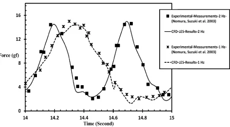
flow with sinusoidal inlet velocity, Figure 2 shows a good agreement between measured drag 4

force from reference [83] and predicted drag force from CFD at two different frequencies (2 Hz 5

and 1 Hz). It can be shown from Figure 2 that the computational model has almost the same 6

behavior of oscillating flow condition as the reference. Table 3 lists the error percentages for each 7

frequency. 8

4.

Analysis and Discussion of Results

9

A multi-suction slot with a certain diameter (𝐷𝑠𝑠) equal to 0.1% [6] from the blade chord at 10

various locations from the leading edge was created, with a shape of NACA0015 with stall angle 11

equal to 13.6 º and Reynolds number equal to 2×105 _{from reference [87, 96, 97], see Figure 3. The}

12

locations for the suction slots were changed in order to obtain an optimum value of 𝐶_𝑇. The test 13

cases investigated were under unsteady flow with non-oscillating velocity at the first to indicate to 14

the best locations and then take the best cases to investigate under sinusoidal wave condition to 15

decide which one has the highest 𝐶_𝑇 and which one has the lowest 𝑆_𝐺. The sinusoidal wave inlet 16

flow boundary condition is having the same specifications as that in the section 3.1 and equation 17

(25). Finally, a comparative analysis was made based on conditions relevant to northern coast of 18

Egypt with different sinusoidal wave frequencies (𝑓 equal to 0.25, 0.167 and 1.25 Hz). 19

4.1 Multi suction slots (Two, Three and Four) 20

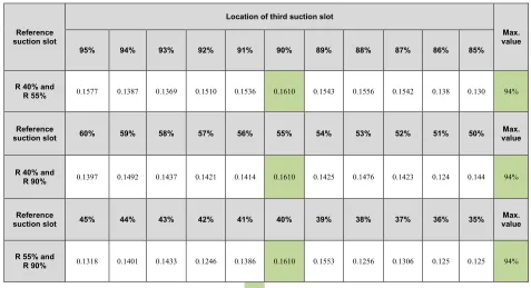
The two suction slots were investigated by making the first suction slots as a reference (𝐿_𝑅𝑠𝑠) and 21

changing the location (x axis direction) of the second suction slots (𝐿_𝑠𝑠) by pitch distance (𝑃_𝑠𝑠) 22

equal to 0.05 at each trial. Considering that, the minimum distance between the two suction slots 23

(∆𝑃𝑠𝑠) was equal to 0.05. 24

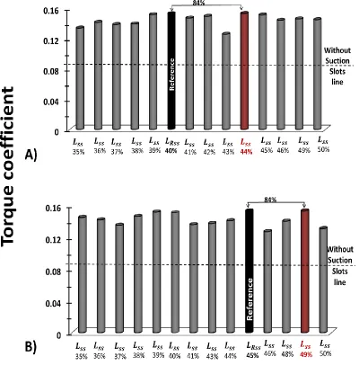
Table 4 provides the details about all two suction slots trial with 𝑃_𝑠𝑠and ∆𝑃_𝑠𝑠 equals to 0.05 to 25

improve the torque coefficient at the stall angle 13.6 º. It can be noted that the 𝐿_𝑅𝑠𝑠 equal to 40% 26

and 𝐿𝑠𝑠 equal to 45% gives a higher torque coefficient than others, where the torque coefficient 27

15

get more improvement in the torque coefficient, the value of 𝑃_𝑠𝑠 and ∆𝑃_𝑠𝑠 was changes to 0.01 1

around the 𝐿_𝑠𝑠 40% and 𝐿_𝑠𝑠 45%. It can be concluded that two suction slots at 𝐿_𝑅𝑠𝑠 40% and 𝐿_𝑠𝑠

2

44% with 𝑃𝑠𝑠 equal to 0.01 give a higher torque coefficient than others by 84% at the stall angle in 3

Figure 4 A). On the other hand, two suction slots at 𝐿𝑅𝑠𝑠 45% and 𝐿𝑠𝑠 49% give also a higher 4

torque coefficient than others by 84% at the stall angle from Figure 4 B). 5

From Table 4 and Figure 4, it can be noted that the three optimum locations for two suction slots 6

were 𝐿_𝑠𝑠40% and 45% with 𝑃_𝑠𝑠 equal to 0.05, in addition to 𝐿_𝑠𝑠 40% and 44% and 𝐿_𝑠𝑠 45% and 7

49% with 𝑃_𝑠𝑠 equal to 0.01. Table 5 demonstrates the effect of the three optimum locations for two 8

suction slots on the torque coefficient at different angles. It can be noted that the two suction slots 9

at 𝐿𝑠𝑠 40% and 45% improve the torque coefficient before the stall by 37.2% and after the stall by 10

95.5%. Also, the two suction slots at 𝐿_𝑠𝑠 40% and 44% improve the torque coefficient before the 11

stall by 33.5% and after the stall by 97.5%. Finally, the two suction slots at 𝐿_𝑠𝑠 45% and 49% 12

improve the torque coefficient before the stall by 36.7% and after the stall by 99%. 13

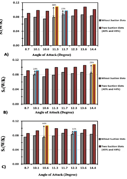
The suction slots have a negative effect on the entropy generation, where the global entropy 14

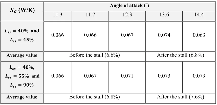
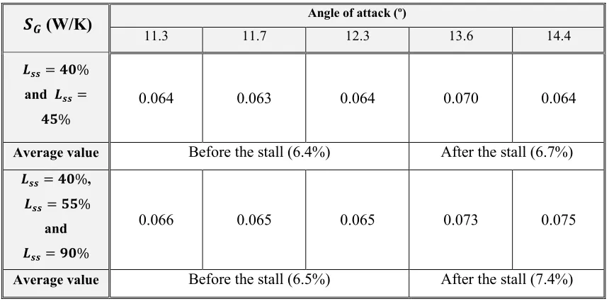
generation rate increases at all angles by 24% before the stall and 23% after the stall due to suction 15

slots at ( 𝐿𝑠𝑠40% and 45%). Where, the 11.3 º angle of attack (before the stall) has the highest 16

difference in global entropy generation rate by 38%. On the other hand, 11.7 º angle of attack 17

(before the stall) has the lowest difference in global entropy generation rate by 13 % due to suction 18

slots at Figure 5 A). Furthermore, the suction slots at ( 𝐿𝑠𝑠40% and 44%) cause increase in the 19

global entropy generation rate value as average for all angles by 21% before the stall and 26% 20

after the stall at Figure 5 B). The 10.1 º angle of attack (before the stall) has the lowest difference 21

in global entropy generation rate by 14% due to suction slots and, the 14.4 º angle of attack (after 22

the stall) has the highest difference by 29 %. Finally, for suction slots at ( 𝐿_𝑠𝑠45% and 49%) at 23

Figure 5 C), the global entropy generation rate increases as average in all angles by 21% before 24

the stall and 22% after the stall. Where, the 10.6 º (before the stall) has the highest difference in 25

global entropy generation rate by 44% and, the 12.3 º (before the stall) has the lowest by 11 % due 26

to suction slots. This phenomenon suggests that the change in velocity gradient due to the suction 27

16

A third suction slot by 𝑃_𝑠𝑠 equal to 0.05 was added to all aerofoils with two suction slots that have 1

higher than 70% improvement in the torque coefficient at the stall angle 13.6 º. Table 6 provides 2

all three suction slots trial with 𝑃_𝑠𝑠and ∆𝑃_𝑠𝑠 equal to 0.05 to improvement the torque coefficient at 3

the stall angle (13.6 º). It can be noted that the 𝐿𝑅𝑠𝑠 equal to 40% - 55% and 𝐿𝑠𝑠 equal to 90% 4

gives a higher torque coefficient than others, where the torque coefficient increases about 94% 5

higher than the aerofoil without suction slot. Therefore, to get more improvement in the torque 6

coefficient, the value of 𝑃𝑠𝑠and ∆𝑃𝑠𝑠 was changes to 0.01 around the 𝐿𝑠𝑠40%, 55% and 90%. From 7

Table 7, it can be noted that no improvement on the torque coefficient by change 𝑃_𝑠𝑠 from 0.05 to 8

0.01 around the 𝐿_𝑠𝑠40%, 55% and 90%. 9

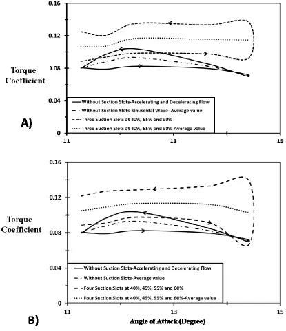
It is clearly noted that the three suction slots at ( 𝐿𝑠𝑠40%, 55% and 90%) improve the torque 10

coefficient before the stall by 35.2% and after the stall by 97%, see Figure 6 A). On the other 11

hand, the global entropy generation rate increases for all angles by 29% before the stall and 25% 12

after the stall as average value at Figure 6 B). Where, the 10.1 º angle of attack (before the stall) 13

has the highest difference in global entropy generation rate by 36% due to suction slots at ( 𝐿_𝑠𝑠

14

40%, 55% and 90%), and the 11.7 (before the stall) and 13.6 (after the stall) º have the lowest 15

difference by 23 %. 16

A fourth suction slot with 𝑃_𝑠𝑠 equal to 0.05 was added to all aerofoils with three suction slots that 17

have higher than 80% improvement in the torque coefficient at the stall angle (13.6) º. Table 8 18

shows the effect of four suction slots on the torque coefficient at the stall angle (13.6 º) with 19

𝑃_𝑠𝑠and ∆𝑃_𝑠𝑠 equal to 0.05 to improvement the torque coefficient. The 𝐿_𝑅𝑠𝑠 equal to 40% - 45% - 20

55% and 𝐿𝑠𝑠 equal to 60% gives a higher improvement in the torque coefficient by 92%. As in two 21

and three suction slots, the value of 𝑃_𝑠𝑠and ∆𝑃_𝑠𝑠 changes to 0.01 around the 𝐿_𝑠𝑠40%, 45%, 55% 22

and 60% to get more improvement in the torque coefficient. From Table 9, it can be noted that the 23

𝐿_𝑠𝑠40%, 45%, 55% and 60% give highest improvement on the torque coefficient with 𝑃_𝑠𝑠 equal to 24

0.01. The four suction slots ( 𝐿𝑠𝑠40%, 45%, 55% and 60%) improve the torque coefficient before 25

the stall by 35.8% and after the stall by 99%, see Figure 7 A). Otherwise, the global entropy 26

generation rate increases by 29% before the stall and 26% after the stall at Figure 7 B).Where, the 27

10.1 º has the lowest difference in global entropy generation rate by 16% and, the 10.6 º has the 28

highest difference by 52 %. The path line coloured by the mean velocity magnitude around the 29

17

effect was very cleared on the separation layers at the trailing edge area and it extends to the area 1

beyond the trailing edge which, leads to delay the stall. Therefore, the NACA0015 with suction 2

slots and Reynolds number equal to 2×105 _{not have the stall condition at 13.6 º. This improvement}

3

can be achieved by two, three or four slots at different location. Where, each case of them has 4

different behaviour. 5

The low pressure areas, at the trailing edge of the NACA0015 without slots, were caused the 6

separation layer. On the other hand, the suction slots affect directly on these areas and decrease 7

from its value and this leads to decrease the separation layers (Figure 9). The difference between 8

the upper and lower surface was decreased by the suction slots and this leads to decrease from the 9

disturbance and the separation layers (Figure 10). The pressure distribution at the upper and lower 10

surface was depending on the number and location of the slots. Therefore, the two, three and four 11

slots were investigated under sinusoidal wave condition in next section. 12

4.2 Optimum location for multi-suction slots based on first law analysis 13

From the previous section, it was noted that there are five scenarios for the suction slots location, 14

which gives higher torque coefficient at the stall regime: 15

1- Two Suction Slots ( 𝐿_𝑠𝑠40% and 45%) with 𝑃_𝑠𝑠 = 0.05 16

2- Two Suction Slots ( 𝐿𝑠𝑠40% and 44%) with 𝑃𝑠𝑠 = 0.01 17

3- Two Suction Slots ( 𝐿_𝑠𝑠45% and 49%) with 𝑃_𝑠𝑠 = 0.01 18

4- Three Suction Slots ( 𝐿𝑠𝑠40%, 55% and 90%) with 𝑃𝑠𝑠 = 0.05 19

5- Four Suction Slots ( 𝐿𝑠𝑠40%,45%, 55%, and 60%) with 𝑃𝑠𝑠 = 0.05 20

In this section, the optimum locations for multi-suction slots based on the torque coefficient were 21

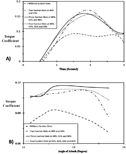
determined under sinusoidal wave condition. Figure 11 compares the torque coefficients for the 22

two suction slots aerofoil at different locations ( 𝐿_𝑠𝑠40% and 45%), ( 𝐿_𝑠𝑠40% and 44%) and 23

( 𝐿_𝑠𝑠45% and 49%). Figure 11 A) illustrates the hysteretic behaviour due to the reciprocating flow 24

which shows a delay in the stall regime and an improvement in the torque coefficient. The two 25

suction slots aerofoil with 𝐿𝑠𝑠 of 40% and 44% has a higher improvement of torque coefficient 26

than that with 𝐿_𝑠𝑠 of 40% and 45% by 6.3% before the stall and 1.5 % after the stall. Moreover, 27

the former aerofoil also has a higher torque coefficient than that with 𝐿_𝑠𝑠 of 45% and 49% by 1% 28

18

Figure 12 shows the effect of adding three suction slots at (𝐿_𝑠𝑠40%, 55% and 90%) and four 1

suction slots at (𝐿_𝑠𝑠40%, 45%, 55%, and 60%) under sinusoidal flow condition on the hysteretic 2

behaviour. From this Figure, it can be noted that in both cases a delay in the stall regime occurred. 3

In addition, the torque coefficient was improved by 26.7% before the stall and 51 % after the stall 4

due to the addition of three suction slots (Figure 12 A). However, the addition of four suction slots 5

resulted in torque coefficient improvement by 25.7% before the stall and 40.5% after the stall 6

(Figure 12 B). 7

From Figure 13, it is clearly noted that adding three suction slots at ( 𝐿_𝑠𝑠40%, 55% and 90%) 8

provided the highest improvement of torque coefficient, from both the instantaneous and average 9

value, compared to all the scenarios that were mentioned in this section. By comparing this 10

aerofoil against the two suction slots aerofoil with optimum locations (𝐿𝑠𝑠40% and 44%), an 11

improvement of torque coefficient of 2.7% before the stall and 22.5% after the stall was observed. 12

Moreover, by comparing the same aerofoil against the four suction slots aerofoil (𝐿𝑠𝑠40%, 45%, 13

55%, and 60%), an improvement of torque coefficient of 1% before the stall and 10.5% after the 14

stall was observed. 15

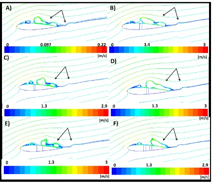
The path-line coloured by mean velocity magnitude highlights the improvement effect of adding a 16

suction slot on the separation layers in Figures 14, 15 and 16. The effect of adding a suction slot 17

on the separation layers at the trailing edge region in Figure 14 (acceleration flow) was small 18

compared with Figures 15 and 16. Where, the separation layers at the area around the trailing edge 19

increased especially at the deceleration flow in the second half of the compression cycle (Figure 20

16). Furthermore, it can be noted that the low pressure areas around the trailing edge decrease due 21

to the slots addition from Figures 17 and 18. The pressure difference between the lower and upper 22

surfaces was decreased as a result of adding the slots. Therefore, the disturbances in the path line 23

at the trailing edge area and the area extended beyond it was decreased. This leads to delay the 24

stall and improve the torque coefficient. 25

Figure 19 shows the effect of adding three suction slots on the boundary layer separation before 26

and after the stall condition via the mean velocity magnitude path-lines. It can be noted that the 27

improvement effect of adding suction slot on separation layers increased in stall regime for both 28

19

for different angles of attack were shown in Figures 20 and 21. Where, the lift column is for the 1

NACA0015 without slots and the right column is for the NACA0015 with three slots at 𝐿_𝑠𝑠40%, 2

55% and 90% with maximum velocity equal to 2.92 m/s. The addition of three slots affects 3

directly the low pressure zones that appear around the trailing edge area and the upper surface of 4

the aerofoil. Where, this low pressure zones were the main reason for the separation layers to be 5

formed. For all angles, the aerofoil with three slots showed an improvement in the pressure 6

distribution and decreased the separation layers especially for the stall angle of 14.4 º in Figure 19 7

I) and J). 8

4.3 EGM method 9

The numerical simulations were used to obtain local entropy viscosity predictions from the 10

different five scenarios for the locations of suction slots. Figures 22 and 23 highlight the 11

comparison between the ( 𝐿_𝑠𝑠40% and 45%), ( 𝐿_𝑠𝑠40% and 44%), ( 𝐿_𝑠𝑠45% and 49%), ( 𝐿_𝑠𝑠40%, 12

55% and 90%) and ( 𝐿_𝑠𝑠40%, 45%, 55%, and 60%). The comparison was provided as an average 13

value for the compression cycle with different angles of attack. From Figure 22 A) it can be noted 14

that the minimum value for the global entropy generation rate occurs with ( 𝐿𝑠𝑠45% and 49%) by 15

20.24% increase in 𝑆_𝐺 before the stall. On the other hand, the minimum value for the global 16

entropy generation rate occurs with ( 𝐿_𝑠𝑠40% and 45%) by 14.54% increase in 𝑆_𝐺 after the stall; 17

see Figure 22 B). Furthermore, the two suction slots ( 𝐿𝑠𝑠40% and 45%) give minimum 𝑆𝐺 as an 18

average value for the compression cycle before and after the stall by 20.5% increase in 𝑆𝐺 value. 19

From Figure 23 it can be concluded that the ( 𝐿_𝑠𝑠45% and 49%) gives the maximum value of 20

second law efficiency by 0.38% before the stall, and, the ( 𝐿𝑠𝑠40% and 45%) gives the maximum 21

value after the stall by 1.19%. Furthermore, the two suction slots ( 𝐿_𝑠𝑠40% and 45%) give 22

maximum value for the second law efficiency as an average value for the compression cycle 23

before and after the stall by 0.72%. The increases in 𝑆_𝐺 (Figure 22) leads to decrease in second 24

law efficiency in some cases than that without suction slots, such as the two suction slots at 𝐿𝑠𝑠 = 25

40% and 𝐿_𝑠𝑠 = 44% before the stall which the second law efficiency decreased by (0.01%), and 26

three suction slots at 𝐿_𝑠𝑠 = 40% , 𝐿_𝑠𝑠 = 55% and 𝐿_𝑠𝑠 = 90% after the stall which the second law 27

20

generation rate values and the second law efficiency due to the different slots number and 1

location. 2

The contours of global entropy generation rate around the NACA0015 at the instantaneous 3

velocity 1.8 m/s for the accelerating (Figure 24) and decelerating flow (Figure 26) in addition 2.92 4

m/s (Figure 25) were represented. Where, the 2.92 m/s was the maximum velocity which create 5

the peak Reynolds number (2×105_{), and 1.8 m/s is approximately at the middle to compare}

6

between the accelerating and decelerating flow. It can be shown that the suction slots have a 7

negative effect on the entropy generation, where the global entropy generation rate increases at the 8

three stages, accelerating flow, maximum velocity and decelerating flow at 13.6 º. The two-9

suction slots at ( 𝐿𝑠𝑠40% and 45%) and ( 𝐿𝑠𝑠45% and 49%) have the lowest difference in global 10

entropy generation rate by 32% at the accelerating flow in Figure 24. Otherwise, the three-suction 11

slots at ( 𝐿𝑠𝑠40%, 55% and 90%) have the highest difference in global entropy generation rate by 12

44 % at the same Figure. However, the global entropy generation rate has lowest difference due to 13

suction slots at the maximum velocity by 28% with the two-suction slots at ( 𝐿_𝑠𝑠40% and 45%). 14

Also, the highest value occurs due to the two suction slots at ( 𝐿_𝑠𝑠40% and 44%) by 35% in Figure 15

25. 16

From Figure 26 it can be noted that the two suction slots at ( 𝐿𝑠𝑠40% and 45%) has the lowest 17

difference in global entropy generation rate by 37% and the highest value occurs due to the three 18

suction slots at ( 𝐿𝑠𝑠40%, 55% and 90%) by 53% at the decelerating flow. Finally, the global 19

entropy generation rate around the NACA0015 without and with suction slots have the highest 20

value at the maximum velocity and the lowest value at the accelerating flow as a general. From 21

Figures 14, 15, 16, and 19 it can be noted that the attached multi-slots to the aerofoil lead to 22

increase in velocity magnitude around the aerofoil, furthermore, it lead also to increase in the 23

entropy generation in Figures 24, 25, and 26. Where, the entropy value depends on the velocity 24

gradient see equation (21). 25

26

4.4 Comparative analysis based on conditions relevant to northern coast of Egypt 27

From the previous section, it can be concluded that the three-suction slots ( 𝐿_𝑠𝑠40%, 55% and 28

21

five scenarios, which give higher torque coefficient. Therefore, these two scenarios were 1

investigated using the oscillating water system based on the real data from the site with different 2

time periods and frequencies (𝑓 equal to 0.25, 0.167 and 1.25 Hz). The hysteretic behaviour due to 3

the reciprocating flow and the total average torque coefficient during the cycle for aerofoil with 4

suction slots at different time periods were shown in Figure 27. It can be concluded that the 5

aerofoil with three-suction slots ( 𝐿_𝑠𝑠40%, 55% and 90%) give higher 𝐶_𝑇 than that with two-6

suction slots ( 𝐿_𝑠𝑠40% and 45%) at 4, 6 and 8 second time period. Also, the increase in time period 7

led to a decrease in the total average torque coefficient in general. At the time period equal to 4 8

second, the aerofoil with two-suction slots ( 𝐿𝑠𝑠40% and 45%) has an average torque coefficient 9

after the stall less than the aerofoil without suction slots by 8.5%. Furthermore, the aerofoil with 10

two suction slots ( 𝐿_𝑠𝑠40% and 45%) with 8 second time period has improvement in the total 11

average torque coefficient before the stall by 17% and after the stall by 8%. 12

Figures 28 and 29 show the instantaneous torque coefficient in addition to average torque 13

coefficient at the accelerating and decelerating cycle for aerofoil with two-suction slots and with 14

three-suction slots. These values were at angle of attack of 13.6 º at different time periods (4 sec, 6 15

sec and 8 sec). It can be seen that the improvement in the torque coefficient has the lowest value at 16

the cycle with time period equal to 4 second. Furthermore, the torque coefficient value and 17

improvement in the torque coefficient at decelerating flow are always higher than that at 18

accelerating flow. 19

The total average torque coefficients during the compression cycle for different angles of attack 20

were shown in Figure 30. It can be observed that for all angles, the suction slot increases the 21

torque coefficient except at the 14.4 º Figure 30 E), where the torque coefficient for the aerofoil 22

with two-suction slots ( 𝐿𝑠𝑠40% and 45%) was lower than that without suction slots by 24% at 23

time period 4 second. Also, the torque coefficient at time period 8 second for the aerofoil with 24

two-suction slots ( 𝐿_𝑠𝑠40% and 45%) was same for that without suction slots. The aerofoil with 25

three-suction slots ( 𝐿_𝑠𝑠40%, 55% and 90%) mostly has a higher torque coefficient than that of the 26

two-suction slots ( 𝐿_𝑠𝑠40% and 45%) at different time period. 27

Tables 10, 11 and 12 show the comparison between the global entropy generation rate before and 28

22

slots ( 𝐿_𝑠𝑠40%, 55% and 90%) at different time periods (4 sec, 6 sec and 8 sec). There were no 1

significant changes in the global entropy generation rate values due to the different time periods. 2

As an average for all time period, the aerofoil with two-suction slots ( 𝐿_𝑠𝑠40% and 45%) has a 3

lower difference in 𝑆𝐺 before and after the stall than the aerofoil with three- suction slots 4

( 𝐿𝑠𝑠40%, 55% and 90%). 5

Suction slots have a negative effect on both the entropy behaviour and the second law efficiency. 6

Therefore, most of cases at Figure 31 have lower second law efficiency for aerofoils with slots 7

than the aerofoils without slots. As it noted in the entropy behaviour, there were also no significant 8

changes in the second law efficiency value due to the different slots number and location. 9

However, the second low efficiency at 14.4 º for the aerofoil with two suction slots ( 𝐿_𝑠𝑠40% and 10

45%) was the highest value at 4, 6 and 8 second by 1%, 2% and 3% respectively, Figure 31 E). 11

The wave cycle with 8 second has the highest value of the second law efficiency as a general. On 12

the other hand, the wave cycle with 6 second has the lowest value. The aerofoil with two-suction 13

slots ( 𝐿_𝑠𝑠40% and 45%) always has higher second law efficiency than that with three-suction slots 14

( 𝐿_𝑠𝑠40%, 55% and 90%) at the different time periods. 15

The flow structures over the NACA0015 aerofoil in oscillating flow was shown in Figure 32 at 16

angle of attack equal to 12.3 º (before the stall) and 14.4 º (after the stall) in Figure 33. The 17

improvement effect of suction slot on flow structures was clear when comparing the NACA0015 18

without and with suction slots, especially in the separated layer regime at the end of aerofoil, 19

which leads to an improvement in the separation regime. 20

5.

Conclusions

21

More than 450 cases were solved to determine optimum location for multi suction slots based on 22

the first and second law of thermodynamics. They aimed to investigate the effect of aerofoil with 23

those optimum parameters on the entropy generation due to viscous dissipation as well as the 24

torque coefficient and stall condition. After that, the comparative analysis based on real data 25

relevant to northern coast of Egypt was applied using the aerofoil with optimum suction slot 26

23

The modeling results show that the optimum locations for two-suction slots aerofoil ( 𝐿_𝑠𝑠 of 40% 1

and 44%), for three-suction slots aerofoil ( 𝐿_𝑠𝑠 of 40%, 55% and 90%), and for four-suction slots 2

aerofoil ( 𝐿𝑠𝑠 of 40%, 45%, 55%, and 60%). The three-suction slots aerofoil with 𝐿𝑠𝑠 of 40%, 3

55% and 90% gives the highest torque coefficient with 26.7% before the stall and 51% after the 4

stall when compared to the aerofoil without suction slots. On the other hand, the two-suction slots 5

aerofoil with 𝐿𝑠𝑠 of 40% and 45% gives the highest second law efficiency by 0.72% compared to 6

the aerofoil without suction slots. The aerofoils with optimum locations for multi-suction slots 7

under conditions relevant to northern coast of Egypt with different wave frequencies were 8

investigated. For NACA0015, adding three-suction slots at optimum locations (𝐿_𝑠𝑠 of 40%, 55% 9

and 90%) mostly gives a torque coefficient higher than that of adding two suction slots at 10

optimum locations (𝐿_𝑠𝑠 of 40% and 45%) for different 𝑡_𝑠𝑖𝑛 (4, 6 and 8 second). However, adding 11

two-suction slots at optimum locations (𝐿𝑠𝑠 of 40% and 45%) always gives a second law 12

efficiency higher than that of adding three-suction slots at optimum locations (𝐿_𝑠𝑠 of 40%, 55% 13

and 90%) for different 𝑡_𝑠𝑖𝑛 (4, 6 and 8 second). 14

The main reason behind the improvement in the torque coefficient after the stall is due to the delay 15

of stall condition. The suction slot increases the torque coefficient and delays the stall angle which 16

further leads to an increase of first law efficiency. On the other hand, it increases the entropy 17

generation rate which leads to decreasing the second law efficiency. The main reason also behind 18

this increase in the entropy generation rate is due to the increases in velocity magnitude around the 19

aerofoil lead to increase also in the entropy generation. Where, the entropy value depends on the 20

velocity gradient. At the present study, the optimization parameters have been varied within a 21

certain range with a fixed increment and all parameter values have been analyzed. An alternative 22

approach that could save time and effort would be to use an automated optimization technique, 23

[98]. Furthermore, Wells turbine impeller using the suction slot with optimum parameters needs to 24

be investigated experimentally in the future. Finally, the operating conditions for the northern 25

coast of Egypt are very suitable for the oscillating system with Wells turbine as a wave energy 26

extractor. So, it is essential that to look at the wave energy in Egypt as the way to reduce fossil 27

24

6.

Acknowledgements

1

The authors would like to acknowledge the support provided by the Department of Naval 2

Architecture, Ocean and Marine Engineering at Strathclyde University, UK and the Department of 3

Marine Engineering at Arab Academy for Science, Technology and Maritime Transport. The 4

authors would like to thank Prof. Mohamed Abbas Kotb for his kind support and guidance. 5

References

6 7

[1] Mamun M. The Study on the Hysteretic Characteristics of the Wells Turbine in a Deep Stall Condition

8

[PhD]. Japan: Saga University, 2006.

9

[2] Rosa AVd. Fundamentals of Renewable Energy Processes. Third Edition ed. United States of America:

10

Elsevier Academic Press, 2012.

11

[3] Falcão AFdO. Wave energy utilization: A review of the technologies. Renewable and Sustainable

12

Energy Reviews. 2010;14(3):899-918.

13

[4] Twidell J, Weir T. Renewable Energy Resources. Second edition ed. New York, USA: Taylor & Francis,

14

2006.

15

[5] Curran R, M. Folley Air turbine design for OWCs. In: Cruz iJ, editor. Ocean Wave Energy. Springer,

16

Berlin. 2008. p. 189-219.

17

[6] Shehata AS, Xiao Q, Saqr KM, Naguib A, Alexander D. Passive flow control for aerodynamic

18

performance enhancement of airfoil with its application in Wells turbine – Under oscillating flow

19

condition. Ocean Engineering. 2017;136:31–53.

20

[7] T. J. T. Whittaker JGL, A. E. Long and M. A. Murray. The Queen's university of Belfast Axisymmetric and

21

Multi-resonant Wave Energy Converters. Trans ASME J Energy Resources Tech. 1985;107: pp. 74-80.

22

[8] T. J. T. Whittaker FAM. Design Optimisation of Axisymmetric Tail Tube Buoys. IUTAM, Symposium on

23

Hydrodynamics of Ocean Wave Energy Conversion. Lisbon,July.1985.

24

[9] Whittaker TJJ, McIlwain, S. T. and Raghunathan, S. . Islay Shore Line Wave Power Station. Proceedings

25

European Wave Energy Symposium. 1993;Paper G6, Edinburgh.

26

[10] Raghunathan S. Theory and Performance of Wells Turbine. Queen's University of Belfast. 1980;Rept.

27

WE/80/13R.

28

[11] Starzmann R. Aero-acoustic Analysis of Wells Turbines for Ocean Wave Energy Conversion [Doctoral

29

]. Germany: Universitat Siegen, 2012.

30

[12] Shehata AS, Xiao Q, Saqr KM, Alexander D. Wells turbine for wave energy conversion: a review.

31

International journal of energy research. 2017;41(1):6-38.

32

[13] IA B. Apparatus for Converting Sea Wave Energy into Electrical Energy. US Patent 3,922,739 1975;2

33

December 1975.

34

[14] Setoguchi T TM, Kinoue Y, Kaneko K, Santhakumar S, Inoue M. . Study on an impulse turbine for wave

35

energy conversion. International Journal Offshore Polar Eng. 2000;10(2):145-52.

36

[15] T. Setoguchi SS, H. Maeda, M. Takao and K. Kaneko. A Review of Impulse Turbine for Wave Energy

37

Conversion. Renewable Energy. 2001;23(2):261-92.

38

[16] T. Setoguchi MT, S. Santhakumar and K. Kaneko. Study of an Impulse Turbine for Wave Power

39

Conversion: Effects of Reynolds Number and Hub-to-Tip Ratio on Performance. Journal of Offshore

40

Mechanics and Arctic Engineering. 2004;126(2):137-40.

25

[17] Okuhara S, Takao M, Takami A, Setoguchi T. Wells Turbine for Wave Energy Conversion —

1

Improvement of the Performance by Means of Impulse Turbine for Bi-Directional Flow. Open Journal of

2

Fluid Dynamics. 2013;03(02):36-41.

3

[18] Raghunathan S. The Wells Air Turbine for Wave Energy Conversion. Progress Aerospace Sciences.

4

1995;31:335-86.

5

[19] Raghunathan S. A methodology for Wells turbine design for wave energy conversion. ARCHIVE:

6

Proceedings of the Institution of Mechanical Engineers, Part A: Journal of Power and Energy 1990-1996

7

(vols 204-210). 1995;209(31):221-32.

8

[20] Dhanasekaran TS, Govardhan M. Computational Analysis of Performance and Flow Investigation on

9

Wells Turbine for Wave Energy Conversion. Renewable Energy. 2005;30(14):2129-47.

10

[21] Brito-Melo A, Gato LMC, Sarmento AJNA. Analysis of Wells turbine design parameters by numerical

11

simulation of the OWC performance. Ocean Engineering. 2002;29:1463–77.

12

[22] Masami Suzuki, Arakawa C. Design Method of Wave Power Generating System with Wells Turbine.

13

Twelfth InternationalOffshoreandPolarEngineeringConference. Kitakyushu,Japan: The International

14

Society of Offshore and Polar Engineers; 2002. p. 527-33.

15

[23] Camporeale SM, Filianoti P, Torresi M. Performance of a Wells turbine in a OWC device in

16

comparison to laboratory tests. the Ninth European Wave and Tidal Energy Conference (EWTEC).

17

Southampton, UK2011.

18

[24] Camporeale SM, Filianoti P. Behaviour of a small Wells turbine under randomly varying oscillating

19

flow. the 8th European Wave and Tidal Energy Conference EWTEC. Uppsala, Sweden2009. p. 690-6.

20

[25] Taha Z, Sugiyono, Sawada T. A comparison of computational and experimental results of Wells

21

turbine performance for wave energy conversion. Applied Ocean Research. 2010;32(1):83-90.

22

[26] Shehata AS, Saqr KM, Shehadeh M, Xiao Q, Day AH. Entropy Generation Due to Viscous Dissipation

23

around a Wells Turbine Blade: A Preliminary Numerical Study. Energy Procedia. 2014;50:808-16.

24

[27] Shehata AS, Saqr KM, Xiao Q, Shehadeh MF, Day A. Performance Analysis of Wells Turbine Blades

25

Using the Entropy Generation Minimization Method. Renewable Energy33-86:1123;2016 ..

26

[28] Christopher Koroneos, Thomas Spachos, Moussiopoulos N. Exergy analysis of renewable energy

27

sources. Renewable Energy. 2003;28(2003):295–310.

28

[29] Shaaban S. Insight Analysis of Biplane Wells Turbine Performance. Energy Conversion and

29

Management. 2012;59:50-7.

30

[30] Soltanmohamadi R, Lakzian E. Improved design of Wells turbine for wave energy conversion using

31

entropy generation. Meccanica, Springer Netherlands. 2015;51(8):1713-22.

32

[31] Miguel AF, Aydin M. Ocean energy: exergy analysis and conversion. The Global Conferance on Global

33

Warming. Lison, Portugal2011.

34

[32] Vosough A, Sadegh V. Different Kind of Renewable Energy and Exergy Concept. INTERNATIONAL

35

JOURNAL OF MULTIDISCIPLINARY SCIENCES AND ENGINEERING. 2011;2(9).

36

[33] Pope K, Dincer I, Naterer GF. Energy and Exergy Efficiency Comparison of Horizontal and Vertical Axis

37

Wind Turbines. Renewable Energy. 2010;35(9):2102-13.

38

[34] Baskut O, Ozgener O, Ozgener L. Effects of Meteorological Variables on Exergetic Efficiency of Wind

39

Turbine Power Plants. Renewable and Sustainable Energy Reviews. 2010;14(9):3237-41.

40

[35] Redha AM, Dincer I, Gadalla M. Thermodynamic Performance Assessment of Wind Energy Systems:

41

An Application. Energy. 2011;36(7):4002-10.

42

[36] Ozgener O, Ozgener L. Exergy and Reliability Analysis of Wind Turbine Systems: A Case Study.

43

Renewable and Sustainable Energy Reviews. 2007;11(8):1811-26.

44

[37] Baskut O, Ozgener O, Ozgener L. Second Law Analysis of Wind Turbine Power Plants: Cesme, Izmir

45

Example. Energy. 2011;36(5):2535-42.