Numerical simulation of Rayleigh-Taylor mixing
Rayleigh-Taylor mixing: direct numerical simulation and
implicit large eddy simulation
David L Youngs
University of Strathclyde, Glasgow, G1 1XJ, United Kingdom
E-mail: [email protected]
Abstract. Previous research into three-dimensional numerical simulation of self-similar mixing due to Rayleigh-Taylor instability is summarized. A range of numerical approaches has been used: direct numerical simulation, implicit large eddy simulation and large eddy simulation with an explicit model for sub-grid-scale dissipation. However, few papers have made direct comparisons between the various approaches. The main purpose of the current paper is to give comparisons of direct nu-merical simulations and implicit large eddy simulations using the same computational framework. Results are shown for four test cases: (i) single-mode Rayleigh-Taylor instability, (ii) self-similar Rayleigh-Taylor mixing, (iii) three-layer mixing and (iv) a tilted-rig Rayleigh-Taylor experiment. It is found that both approaches give similar results for the high-Reynolds number behavior. Direct numerical simulation is needed to assess the influence of finite Reynolds number.
1. Introduction
Rayleigh-Taylor (RT) instability plays an important role in many areas of research. It can degrade the performance of inertial confinement fusion capsules, see for example Amendtet al(2002). It also occurs in many astrophysical flows, see for example Fryxellet al(1991). The simplest case consists of fluid with density1resting initially above fluid with density2<1in a gravitational fieldg. Experiments using incompressible fluids with low viscosity, low surface tension and ran-dom initial perturbations have shown that the ran-dominant length scale increases as mixing evolves. If mixing is self-similar then dimensional reasoning suggests that the length scale should be pro-portional togt2. The experiments indicate that the depth to which the mixing zone penetrates the denser fluid , generally known as the bubble distance, is given by:
2 2
1 2
1 2
b
h g t A g t (1)
where varies slightly with Atwood number,A, and is typically in the range 0.04 to 0.08. The distance to which the mixing zone penetrates the lighter fluid is referred to as the spike distance,
s
h
. The ratioh / h
s bis a slowly increasing function of the density ratio
1/
2. Three-dimensional numerical simulation of this self-similar turbulent mixing problem, and some more complex ex-tensions of the simple case, is the subject of the present paper.here that high-resolution large eddy simulation is the most computationally efficient way of cal-culating the high-Re behavior and that this approximation is needed for the more complex situa-tions in which RT mixing occurs. As the problems of interest have an initial discontinuities, ILES (implicit large eddy simulation) is strongly favored. However, a few researchers have used LES (large eddy simulation) with explicit models for the dissipative processes. Mixing of miscible flu-ids is considered here and for ILES or LES to be valid the Reynolds number is assumed to be high enough for the flow to be beyond the “mixing transition” where, according to the hypothesis of Dimotakis (2000), the Schmidt number does not affect the amount of molecular mixing.
Section 2 reviews previous research on 3D numerical simulation of RT mixing, both DNS, ILES and LES. The emphasis is on the simple incompressible situation (1). The choice of numerical technique is a matter of considerable controversy. However, very few papers have made direct comparisons between the various approaches. The main purpose of the current paper is to give some direct comparisons of DNS and ILES results using the same computational framework. The emphasis is on quantities which are of most importance in practical applications, such as ICF: the extent to which to which the fluids mix and the degree to which mixing occurs at a molecular level. Section 3 summarizes the numerical method used here for both DNS and ILES. Results for four test cases: (i) single-mode RT instability, (ii) self-similar RT mixing, (iii) three-layer mixing and (iv) a tilted-rig RT experiment are given section 4. Concluding remarks are given in section 5.
The present paper focuses on 3D numerical simulation of RT mixing, which has been feasible since the 1990s. Other aspects of research into RT instability have been reviewed by various au-thors. For example, Sharp (1984) gives a review of the early research into Rayleigh-Taylor insta-bility. Kull (1991) , Abarzhi (2010), Abarzhi and Rosner (2010) give reviews of theoretical mod-elling approaches. Low Atwood number experiments, for which detailed diagnostics are feasible, are reviewed by Andrews and Dalziel (2010). Wide-ranging reviews of many aspects of the insta-bility processes are given in the theme issue of the Philosophical Transactions of the Royal Soci-ety edited by Sreenivasan, Gauthier and Abarzi (2013).
Much of the content shown here was presented at the “Turbulent Mixing and Beyond” workshop held in 2014. The paper addresses key themes and topics of the TMB program, in particular non-equilibrium turbulent processes, Rayleigh-Taylor instabilities and interfacial mixing.
2. Summary of previous work on numerical simulation of Rayleigh-Taylor mixing
confirmed that the observed growth rates are likely to be influenced by initial conditions. By use of a simple model, Dimonte (2004) argued thatshould have a weak (logarithmic) dependence on initial perturbation amplitudes. This explains whydoes not vary greatly within a series of experiments using the same apparatus.
Cook and Dimotakis (2001), Cook and Zhou (2002) and Younget al(2001) performed the first DNS for RT mixing and gave results for the early stages of the mixing process and the detailed structure of the mixing zone. Cooket al(2004) used LES with 11523meshes and an explicit dis-sipation model. Both of these approaches showed the development of a “mixing transition”, as defined by Dimotakis (2000), when an inertial range begins to form. The LES gave~0.027, very similar to the ILES results of Dimonteet al.(2004). Ristocelli and Clark (2004) used DNS to un-derstand the time variation ofin the early stages of the mixing process. Subsequently very high resolution DNS results, using 30723meshes, were given by Cabot and Cook (2006). This paper showed that was high early in the simulation and the dropped to a low value after the mixing transition. The value ofthen slowly increased to ~0.025 by the end of the simulation, when
/ b b
Re h h , reached 3104, close to the values obtained from the previous ILES/LES. The At-wood number used in these papers did not exceedA=0.5. A form of LES was also used by Burton (2011) to perform simulations at high Atwood number, A=0.5 to 0.96. In all cases, a low value of ~0.02 was obtained. The spike to bubble ratio, hs/hb, was estimated and found to be signifi-cantly less at high Atwood number than reported for the immiscible-fluid experiments of Dimonte and Schnieder (2000). The review paper, Statsenkoet al(2013), shows results for the total mixing zone width at density ratios 3:1 to 40:1. The results at 3:1, assuming hs~hb, indi-cate~0.03. High resolution (up to 4032x40962) DNS results for RT mixing at a range of At-wood numbers ,A=0.04 to 0.9 have given by Livescuet al(2010,2011) and a review of DNS ap-proaches is given by Livescu (2013). All the calculations referred to so far (DNS, ILES, LES) have indicated low values of~0.02 – 0.03 for mixing of miscible fluids arising from ideal ini-tial conditions.
It appears thatonly has a unique value, corresponding to loss of memory of the initial condi-tions, if small random short wavelength perturbations are assumed. The best estimate is then ~0.025 with little dependence on Atwood number. However, some doubt still remains. Cabot and Cook (2006) have speculated that there might be a difference in the behavior at ultra-high Reyn-olds number, beyond present computational capabilities.
the use of front-tracking simulations in such cases and expressed concern about the treatment of molecular mixing in the ILES approach. The paper by Glimmet al(2013) uses front tracking and LES to model a range of experiments, many of which have used immiscible liquids. Initial condi-tions were estimated, from the early-time experimental photographs in some cases, and good agreement was obtained with the observed growth rates which had values ofin the range 0.05 to 0.08. For turbulent mixing experiments with random initial perturbations, initial conditions are never known precisely. However, it is clear that several authors have achieved improved agree-ment with experiagree-ment by estimating the initial conditions as accurately as possible.
Since Youngs (1994), TURMOIL ILES have been performed with increasing mesh resolution. In Youngs(2003) the mesh resolution was increased to 720 x 480 x 480. For random short wave-length initial perturbations the value ofwas 0.027, in agreement with the earlier simulations. Inogamov (1978) pointed out that self-similar mixing at an enhanced rate could be obtained if random long wavelength perturbations with amplitudewavelength, which corresponds to ak-3 power spectrum. It was found that if such a perturbation spectrum was used with a very small am-plitude standard deviation of only 0.00025the computational domain width, thenwas in-creased to about 0.06, a typical experimental value. Similar results using inin-creased resolution were given in Youngs (2009). In Youngs (2013) ILES results were shown for mesh resolutions ~2000 x 1000 x 1000. The increase in mesh resolution had little effect on the low value of ob-tained when short wave length initial perturbations are used. A range of calculations was carried at different density ratios and with different levels of thek-3– spectrum perturbations, giving a range of values of~0.025 to 0.1. Properties of the mixing zone were derived as functions of.
In this section emphasis has been given to the values ofcalculated by various researchers and to the agreement with experiment. An important conclusion is that there is a large difference be-tween the mixing rates for simulations using ideal conditions and those observed experimentally. The papers referred to here have also given many results for the detailed structure of the mixing zone. There has been some experimental validation of this. However, as regards the detailed structure, simulations have provided much more information than can be obtained experimen-tally.
Several papers have considered simple extensions to the self-similar mixing case (1). ILES results for a three-fluid mixing problem were given Youngs (2009) and further results for this case are shown here in section 4. In Andrewset al(2014) the initial interface was tilted relative to the di-rection of gravity; DNS, incompressible and compressible ILES results were given. In section 5 here further comparisons of DNS and ILES are shown for this case. RT mixing in a tall tube was considered by Lawrie and Dalziel (2011) and ILES was compared with a simple model which predictedhb~t2 / 5. Williams (2017) has used ILES (TURMOIL) for RT mixing with non-uni-form stratification in each fluid. Variable acceleration, withgalternating in sign was investigated by incompressible ILES, Dimonteet al(2007) and Ramaprabhuet al(2013). Alternating sign ac-celeration and evolution of RT mixing with an additional localized perturbation was considered in Statsenkoet al(2013). In the paper by Olsonet al(2011) initial shear is added to investigate the combined effect of Rayleigh-Taylor and Kelvin-Helmholtz instabilities. This paper also compares results for DNS and LES with an explicit dissipation model. It is shown that the LES results con-verge to the DNS result at high resolution.
(2013). Use of a simple approach is considered here, a 2nd/3rdorder Lagrange-remap method (TURMOIL). It is argued that this method is suitable for relatively complex problems with initial density discontinuities and shocks. Rehagenet al(2017) gives a comparison of a similar La-grange-remap technique with the high-order method of Cabot and Cook (2006), for RT mixing at moderate mesh resolution. Agreement between the two numerical techniques was found for global quantities such as mixing zone widths and the degree of molecular mixing. In these simu-lations the dissipative scales were well resolved at the start of the calculation (near DNS) but at the end the simulations were effectively LES. A more advanced LES approach, the stretched-vor-tex subgrid-scale model, has been applied to RM mixing, Lombardiniet al(2011), but has not been used for the RT mixing problems considered here. A wide range of numerical techniques is available. However, the most appropriate choices for simulating the variety of RT and RM mix-ing cases is very complex problem and additional studies are required to resolve this challengmix-ing issue.
3. Summary of the numerical method used
The results shown here have been obtained by using the TURMOIL Lagrange-remap hydrocode which calculates the mixing of compressible fluids. This was initial used for ILES of RT mixing, Youngs (1991) and solved the Euler equations plus advection equations for fluid mass fractions. More details of the Lagrange-remap method, its application to RT and RM mixing and further discussion of ILES techniques are given by Grinsteinet al(2007). The remap phase uses the mon-otonic advection method of van Leer (1977) to prevent spurious oscillations. In turbulent flows, the monotonicity constraints provide the required dissipation at high-wavenumbers and this is the basis of the ILES approach. Perfect gas equations of state are used for each fluid species with constant values of the specific heat ratio, r, and specific heat ,cvr. The mixture is assumed to be in pressure and temperature equilibrium. The pressure of the mixture is then given by
1
with r vr r/ vr rr r
p e
c m
c mFor DNS the Navier-Stokes equations are used and include the effects of viscosity (kinematic viscosity), species diffusion and heat conduction. Simplified material properties are used. The same diffusivity,D, is used for all fluid species and for heat (i.e. the conductivity coefficient is c Dp ). This leads to a simplified form of the equations , previously used byKokkinakiset al(2015), for density,, velocity, ui, mass fractions, mr and specific internal energy,e
:-
0
with 2 , where is the deviatoric strain rate j j
i j ij
i
i
j i j
ij ij ij
r j
r r
j i j
j j
j j i j
u
t x
u u S
u p
g
t x x x
S e e
m u
m m
D
t x x x
eu u
e h
p D
t x x x x wherehe=enthalpy
For ILES the Euler equations are used;and D are set to zero. For the calculations shown here, the adiabatic constants are 1 25 / 3and the specific heats are chosen to give temperature equilib-rium initially at the unstable interface: 1 v1c 2 v2c (specific heats are only needed for the calcu-lation of volume fractions –see below). Heat conduction does not have a significant effect. For DNS the Schmidt number is unity, i.e.= D, as in many previous RT DNS. The initial interface pressure is set to a sufficiently high value to give a peak Mach number less than 0.2 and this gives near incompressible flow for which mean volume fraction distributions are unaltered by increase in pressure. Hence the results shown are representative of incompressible gaseous mixing.
In the numerical method, the Lagrange and remap phases are unchanged for DNS. In particular, monotonic advection is retained in the remap phase. Extra steps in the calculation are included for viscosity and diffusion of mass fractions and enthalpy. For accurate DNS, the viscous and diffusive scales need to be well enough resolved for dissipation in the remap phase to be negligible.
A convenient way of quantifying the extent to which speciesrmixes with the other fluids is by use of the mixed mass, Zhouet al(2016)
21
r
mr m dVr Mr
m dVrM (3)
Mrdenotes the total mass of fluidrwhich remains constant. Hence the production ofMrcorresponds to the dissipation of mr2.
The amount of mixing which occurs in the diffusion steps (the resolved mixing) can be calculated from res r 2 r r j j m m D dVdt x x
MFor accurate DNS,Mr Mrres. However, as some mixing will occur in the remap steps,MrMrres . A measure of the accuracy of the DNS is given by the ratio
res
r r
r
r
M M
M (4)
An alternative approach would be to use a non-dissipative remap phase. The resolution would need to be sufficient to make any deleterious effects due to spurious oscillations negligible and it is thought that this would be difficult to quantify. The advantages of the approach chosen here is that a robust computational method is retained and a method of checking the accuracy of the DNS is available. A similar check on viscous dissipation is also made; for accurate DNS, the loss of kinetic energy in the remap phase should be small compared to the dissipation directly due to viscosity.
For quantifying the amount of mixing that takes place, it is useful to construct fluid volume frac-tions
1 1
r vr r
r
s vs s
s c m f c m
(1 ) (1 ) r r r r r f f f f (5) (1 ) (1 ) r r r r r
f f dV
f f dV
(6)In general, the overbar denotes the ensemble average. For the cases shown here the ensemble av-erage is approximated by using plane averaging sections 4.2 and 4.3) or line averaging (sub-section 4.4). If only two fluids are present, 1 2and 1 2 . The values of the molec-ular mixing parameters vary from 0 (no molecmolec-ular mixing) to 1 (fully mixed at a molecmolec-ular level).
As explained by Youngs (2007) the spatial variation of the dissipation in TURMOIL ILES can be accurately quantified. The Lagrange phase is non-dissipative in the absence of shocks as in the test cases considered here. The remap phase is split into separate steps forx,yandzadvection. Consider thex-remap of a quantityper unit mass. The equations solved are
0 0 u t x u t x These equations imply
2 20 u t x
Hence in the absence of numerical dissipation
2dVshould be conserved in the remap step. However, if monotonic advection is used for, dissipation of this quantity will occur. The spatial distribution of the dissipation can be derived as follows. Suppose the difference equations for con-servation of mass andare written as1 1
2 2
1 1 1 1
2 2 2 2
1 1 1
2 2 2
1 0
1 1 0 0
0 1
where and are the cell masses at the start and end of the step, is the mass flux accross the cell boundary and
j j j j
VL VL
j j j j j j j j
j j
j j j
M M M M
M M M M
M M
M x x VL is a van Leer limited value of .
These difference equations are used to calculate the reduction in
2dV. The summation is re-arranged to give
1 12 2
2 2
0 0 1 1
j j j j j j
j j
M M M
The contribution to the dissipation, 1 1
2 2
j Mj
, is then divided between meshes j andj1. If is set to each of the velocity components in turn, this technique gives the spatial distribution of the dissipation of kinetic energy in the remap phase. For the ILES this gives the “sub-grid-scale” energy dissipation. Further details are given in Youngs (2007). This idea was first used by DeBar (1974) to calculate kinetic energy loss, but not in the context of turbulence simulation. If is set tomr, the dissipation calculated corresponds to the production ofMr(3).
The TURMOIL method used second-order accurate numerics in the Lagrange phase and third-order monotonic advection in the remap phase. Second-third-order, central differencing is used for the viscous and diffusion terms. As noted in section 2, high order methods have, as a rule, been used in previous DNS studies of RT mixing. Comparisons between TURMOIL and higher order meth-ods, typically of order 5, for a simple viscid vortical flow are given inShanmuganathanet al(2014) andTsoutsaniset al(2015). TURMOIL compares very favorably with the higher order methods. It does require a finer mesh (by a factor ~1.5 ) to obtain converged results but is computationally much faster. Hence it is considered a feasible approach for DNS.
4. Applications
4.1 Single Mode Rayleigh-Taylor instability
The first application is single mode Rayleigh-Taylor instability at density ratio 1/ 2 20and withAg=1. The width of the domain, set to unity here, is twice the perturbation wavelength,, and the kinematic viscosity (the same for each fluid) is chosen so that the most unstable wave-length (if diffusivity is neglected) is
1/ 3 2
1
m 4 2
v Ag
(8)
Diffusivity, with D, also reduces the growth rate of short wavelength perturbations. How-ever, the parameter mis nevertheless considered to be a useful estimate of the viscous/diffusive scale. The Mach number of the simulations is sufficiently low to give near-incompressible flow. There is initially a sharp interface but this quickly becomes diffuse. Numerical results are shown in figure 1.
(a) (b) (c) (d)
[image:8.595.88.480.533.685.2]Volume fraction contours ( f10.1,0.3,0.7,0.9) for three different mesh sizes are compared at t=2.5. Figure 1(a) shows results at an earlier time with viscosity and diffusivity omitted. This clearly shows that viscosity and diffusivity have a large effect. The effect of viscosity and diffu-sivity is accurately calculated with m 32 the mesh size,x, figure 1 (d). However, a good ap-proximation is obtained with m 8 x, figure 1 (b). In that caseas defined by (4) is 0.07 and this implies that some of the mixing occurs in the remap phase. It is concluded that the influence of diffusivity on the amount of mixing is adequately calculated with less than fully resolved DNS.
4.2 Self-similar mixing at a plane boundary
One of the ILES calculations described in Youngs (2013) is repeated with viscosity and diffusiv-ity included. For the case chosen, high-densdiffusiv-ity fluid,
120
, occupies the regionx< 0 and the low density fluid,
21
, occupies the regionx> 0. Gravity acts thex-direction and is chosen to giveAg=1. Within each initial fluid, hydrostatic equilibrium with an adiabatic variation is used. Short wavelength random perturbations are used with wavelengths in the range 4xto 8x. The resolution used for the DNS is same as that used for the ILES, 1550x1000x1000 meshes. The width of the domain in theyandzdirections is unity. For viscosity and diffusivitya constant D
and the value of the constant is chosen so that the viscous scale, (8), is 17meshes
m
. Then, according to the results of the previous sub-section, the early time effect of viscosity and diffusivity should be well resolved. However, the dissipation scales also need to be resolved at later times when turbulence develops. For homogeneous turbulence dissipation occurs at the Kolmogorov scale,K, which is related to, the kinetic energy dissipation rate per unit mass by
1/ 4 3
K
For RT mixing, experiments and simulations, Dalziel et al (1999), Cabot and Cook (2006) show high wavenumber spectra similar tok-5/3. Hence a similar scaling law for the dissipation scales (at least atSc~1) is expected. For self-similar RT mixing,is proportional to potential energy loss rate per unit mass, ~ Aghb and this implies that the dissipation scales should decrease slowly with time,K ~hb1/ 8. Hence the need to resolve the turbulent dissipation scales will eventually deter-mine the mesh resolution required.
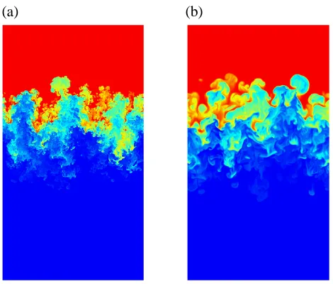
(a) (b)
Figure 2: Volume fraction distributions for plane sections, denser fluid at top; (a) ILES att=3.0, (b) DNS att=3.2.
[image:10.595.143.450.390.607.2]The main purpose of this section is to compare results for the amount of molecular mixing, as de-fined by the parameters(5) and (6). Figures 3 and 4 compare the ILES and DNS results.
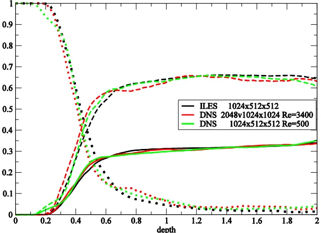
Figure 3: Profiles of dense fluid volume fraction (solid lines) and molecular mixing parameter (dotted lines)
Figure 3 shows values of f1and plotted against the scaled distance variable x W/ where
1 1 1
W
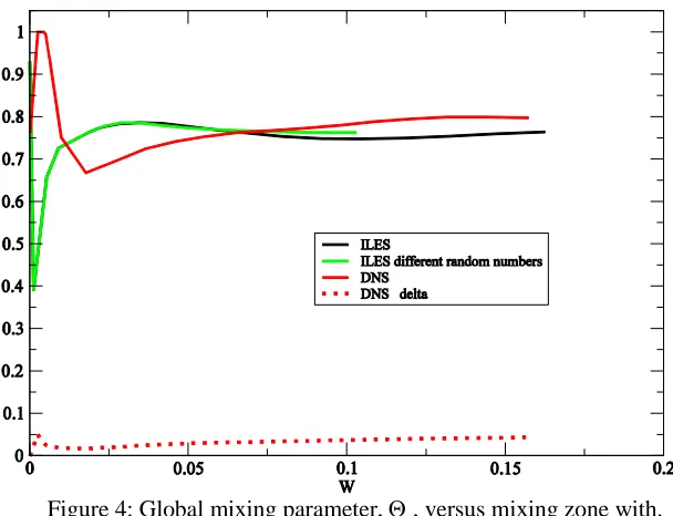
f f dx is an integral measure of the mixing zone width. It is evident that DNS and ILES give very similar results. The two ILES results shows that there are small differences in re-sults due to the choice of random numbers for the initial perturbations.Figure 4: Global mixing parameter, , versus mixing zone with.
Figure 4 shows that at the end of the simulations, the global mixing parameter reaches very simi-lar values, ~ 0.75 0.8 , for DNS and ILES. However, the early time behavior is different, At the start of the DNS, is close to unity when the initially sharp interface diffuses away and then drops to a lower value as the instability evolves. Finally, as small scale structure develops, rises to a limiting value of about 0.8. This is, of course the physically correct behavior for the chosen values ofandD. Figure 4 also shows a plot of the quantity, as defined by equation (4). This never exceeds 5% and this indicates that the DNS is adequately resolved. For the ILES there is initially a sharp dip in as the instability evolves without the development of fine scale structure. Then, when sufficient fine scale structure (inertial range) can be resolved, rises to a limiting value of 0.75 to 0.8. In this case, the early time behavior is determined by the numerics; the ILES results for the degree of molecular mixing are only meaningful when the late-time limiting value is approached. This occurs whenW~0.02. The width of the mixing zone, ~8W according to figure 3, is then equal to 160 times the mesh size. For the DNS higher resolution is needed to reach the limiting value of The dynamic range is not very high in the DNS shown here but should be sufficient to estimate the limiting value of s a limiting value has been reached, it is consid-ered appropriate to describe the flow as “turbulent” by the end of the simulation. The dynamic range is not high enough to calculate the high-Reynolds behavior of some of the fine-scale prop-erties.
The molecular mixing parameter,, varies from=0.6 on the bubble side to=0.95 on the spike side for both DNS and ILES; this is in good agreement with the DNS results of Livescuet al (2011). The spike/bubble ratio hs/hb1.7is also the same for both DNS and ILES and in agree-ment with previous results, for example Burton (2011).
An appropriate estimate of the Reynolds number, based on the bubble distance and velocity, is
2
Re h hb b ~ hb Aghb 2500 at the end of the simulation
The Reynolds number achieved is close to that in the RT experiments described by Mueschkeet al(2009) in which reaches a plateau level for gaseous mixing atSc~0.7. For water channel ex-periments,Sc~1000, a significantly higher Reynolds number, probably of order 104(not achieved in the experiments) is needed to reach the plateau level. This highSccase is beyond current DNS capability.
The comparison of the DNS and ILES results leads to the following conclusions. The two ap-proaches give very similar results for the late-time degree of molecular mixing, when a high Reynolds number is achieved. This should dispel concerns about the ability of ILES to calculate molecular mixing. If the high Reynolds number behavior of the global properties of the mixing zone is the main point of interest then the ILES approach is able to estimate this with significantly less computer resources than DNS. If the influence of finite Reynolds number is required then DNS is, of course, essential. Moreover, DNS is required for many small scale properties of the mixing zone.
4.3 Three-fluid mixing
In this sub-section a more complex RT mixing problem is considered: the break-up of a dense fluid layer. In some ICF capsule designs, for example Amendt et al (2002), multiple shells are used and this has provided the motivation for a three-layer test case. This is significantly more difficult than the previous test case. For self-similar mixing at a plane boundary the main require-ment is to reach the self-similar state before the end of the simulation. For the three-fluid case, turbulent flow needs to established before the intermediate layer breaks up, and for DNS this has proved difficult. It would be desirable to show DNS for significantly higher Re than has been possible at present. Nevertheless, some interesting results for the influence of viscosity on the break-up of the dense layer are given.
DNS results are given for one of the cases for which ILES results were given in Youngs(2009) . The initial configuration, withxmeasured downwards in the direction of gravity has
1
1 2
1
2 2
3
Fluid 1: 0 density
Fluid 2: density
Fluid 3: 2 density
x H
H x H
H x H
A range of density ratios was considered in Youngs (2009). For the comparisons shown here 2/ 1 2/ 3 3
is chosen. Gravity is chosen to giveAg=1 andH=1 here. Results are given as a function of a scaled time Ag H t/ . Initial random long wavelength perturbation are added at the lower unstable boundary with a power spectrum given by
3 1
2
/ 4 2 /
( )
0 otherwise
C k x k H
P k
The value of C was chosen so that the standard deviation of the initial perturbation was 0.00025H
. For ILES this gave approximate self-similar growth, before dense layer break-up, with an enhanced value of~ 0.06, a typical experimental value.
diffusive scales at early time was similar to that obtained in the last sub-section. A convenient es-timate of the Reynolds number for the flow is
1 2 1
2
Re h hb b when hb= width of dense layer, H H AgH
This gives Re ~ 500, 1400, 3400 for the three DNS mesh sizes. For the lowest value of Re~500 the calculation has been repeated using the intermediate mesh size, thus giving m 32 x, to show the effect of mesh size at given Re.
Calculations are run to=10, when the amount of mixing is close to the final value. Figures 5 and 6 show volume fraction distributions for the ILES and the highest resolution DNS. It is evident that the overall time scale for the mixing process is very similar for the two calculations. How-ever, more fine-scale structure is present in the ILES, in spite of the lower resolution.
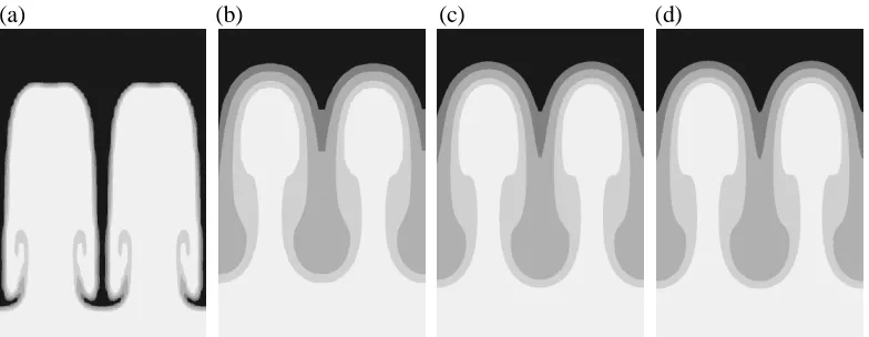
(a)=1 (b)=2.5 (c)=4 (d)=10
(a)=1 (b)=2.5 (c)=4 (d)=10 Figure 6: Dense fluid volume fraction (plane sections) for DNS, 2048x1024x1024 meshes, Re=3400
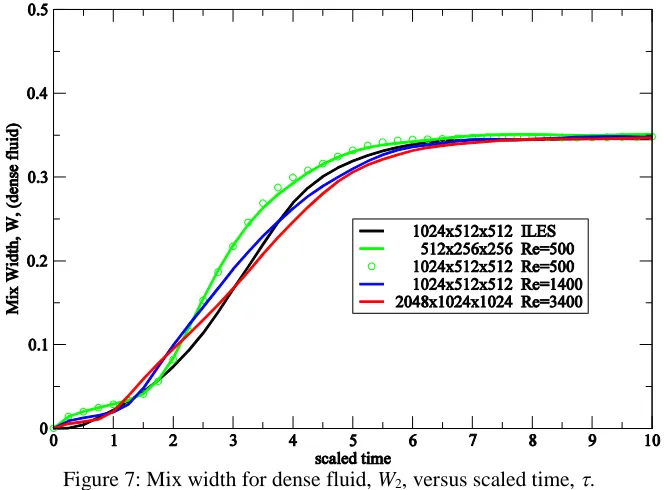
Figure 7: Mix width for dense fluid,W2, versus scaled time,.
Figure 7 shows the evolution of the integral mix width for the dense fluid layer,
2 2 1 2
Distributions of volume fractions averaged over (y,z) –planes are shown in figures 8 and 9. At =4, the distributions for the highest Re DNS and the ILES are very similar. This is also true for the final state at=10. It is interesting to note that for the final state, figure 9, the effect of Reyn-olds number is surprisingly small.
Figure 8 : Plane averaged volume fraction distributions at scaled time=4, dotted lines : f1, solid lines :f2, dashed lines :f3.
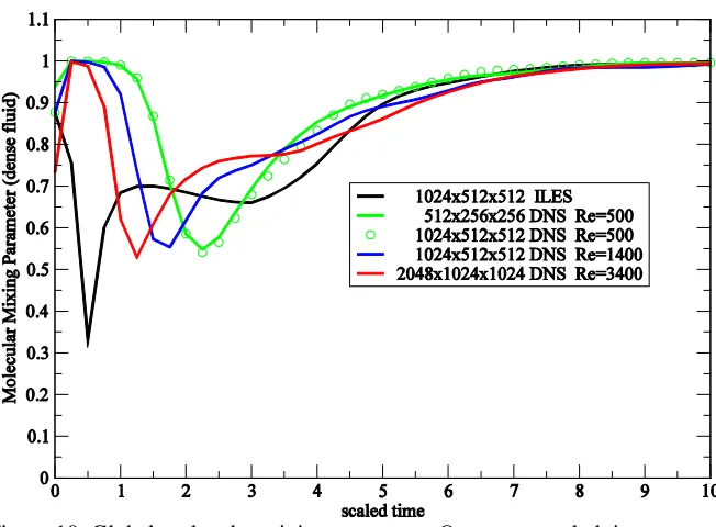
[image:15.595.139.456.461.691.2]Figure 10: Global molecular mixing parameter,versus scaled time,
Figure 10 shows the evolution of2, the global mixing parameter for the dense fluid, as defined by (6). The DNS results show that the Reynolds number has a significant effect. As for the two-fluid mixing case (sub-section 4.2) the interface initially diffuses away and gives values of2 close to unity. Then as mixing evolves2drops to a value of ~0.55 and finally rises as fine scale structure develops. The minimum value changes little with Reynolds number but time at which the minimum occurs increases as viscosity increases. For high Reynolds number self-similar mix-ing,2should reach a plateau level, as implied by figure 4. For the range of Reynolds numbers considered here this is not achieved before mixing reaches the top of the dense layer at~ 3. Hence DNS at considerable higher Reynolds number is needed to model the high-Reynolds num-ber behaviour. For the ILES a plateau level of2~0.68 is reached for=1 to 3 and this is typical of experimental results for Sc~1,Mueschkeet al(2009) , which indicate~0.70.
The conclusions drawn from the DNS and ILES results for the three-fluid test case are as follows. The overall progress of the mixing process, as indicated for the volume fraction distributions, is very similar for the ILES and the highest resolution DNS. The ILES appears to give an adequate approximation to the high-Re behavior. DNS is able to assess the influence of viscosity at moder-ate Reynolds number and at Schmidt number Sc~1.
4.4 A tilted-rig Rayleigh-Taylor experiment
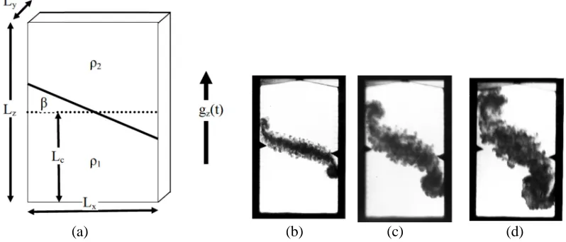
The final problem considered is the Tilted-Rig test case described by Andrewset al(2014). This is based on an experiment described by Youngs (1989) for which a tank containing hexane (top, g/cc) and NaI solution (bottom,=1.89g/cc) was accelerated downwards. The experi-mental rig was inclined at an angle=546to the vertical. This tilted the initial interface relative to the sides of the tank and led to a large scale overturning motion in addition to the growth of a turbulent mixing zone. This flow is, on average, two-dimensional and the main purpose of the test case is to provide a benchmark problem for 2D RANS (Reynolds-Averaged Navier-Stokes) mod-els and was used for this purpose by Denissenet al(2014). It is a challenging test case for DNS; the viscosity used both here and by Andrewset al(2014) needs to be increased by a factor 10 in order to resolve the dissipation scales.
In the simulations, figure 11(a), the tank is static and a gravitational force is applied in the vertical direction. The domain size used in the simulations is Lx Ly 15cm,Lz24cm . Reflective boundary conditions are used in thexandzdirections. Periodic boundary conditions are used in theydirection. The value ofLyis increased from the experimental value of 2.5cm in order to re-duce fluctuations fory-averaged quantities.
[image:17.595.107.506.409.580.2](a) (b) (c) (d)
Figure 11: The Tilted-Rig experiment. (a) schematic, (b),(c),(d) sequence of experimental images at times 45.3ms, 59.8ms, 71.1ms.
In the experiment the acceleration takes about 20ms to rise to a near-constant plateau level. The incompressible ILES and DNS reported in Andrews et al. (2014) used the measured acceleration history forgz(t). However, for the compressible TURMOIL simulations this was impractical and a constant value of gz=0.035 cm/ms2 was used. A correction was made to the time scale for com-parisons between the simulations. Results are given here for a scaled time of
2.117
z x
Ag t L
which corresponds approximately to figure 11(d).
The DNS of Livescu, shown in Andrewset al.(2014) began with a slightly diffuse interface. Moreover, as the simulations began withgz=0, the interface further diffused away before the in-stability evolved. This led to a significant delay in the development of the inin-stability. The TUR-MOIL DNS results with constantgzand a sharp initial interface reduce this effect and it is argued that this gives a more direct comparison of ILES with DNS.
The mesh sizes used for the TURMOIL simulation shown here are 600 x 600 x 960 (ILES) and 1600 x 1600 x 2560 (DNS). The value used for=Dwas, 1.57 x 10⁻⁴, the same as the lowest value used by Livescu. Then for the DNS m 15 x and the resolution of the early stages is sim-ilar to that in the previous sub-sections. As described in Andrewset al(2014), random initial per-turbations have ak-2power spectrum with wavelength range 0.2 to 7.5cm and standard deviation 0.0075cm . Calculations with the same initial perturbations but without the tilt give~0.05, typi-cal of the experimental values.
Two estimates of the Reynolds number for the DNS are give. Andrewset al.(2014) used a value base on the maximum perturbation wavelength, max 7.5cm
:-max max
Re / 14000
1 Ag
A
The Reynolds number based on the bubble distance and velocity (measured in the center of tank) at the time selected, t=2.117, is approximately
Re h hb b 2400
and this is similar to the value achieved for DNS shown in section 4.2
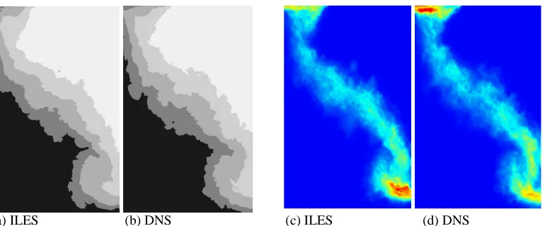
(a) ILES (b) DNS (c) ILES (d) DNS
Figure 12: (a,b) distributions of volume fraction (contours for f10.025, 0.3, 0.7, 0.975) and (c,d) turbulence kinetic energy,k(range =0 to 0.05 cm2/ms2)
[image:18.595.94.479.470.630.2]
2 2 2
where x x y z z
x z
x z
u u u u u u u
k u , u
[image:19.595.91.377.107.146.2]The ILES and DNS give very similar distributions. The width of the mixing zone is slightly greater in the DNS. As for the three-layer problem, this is attributed to reduced fine-scale mixing in the early stages of the DNS which gives greater density contrast and increased buoyancy.
Figure 13 shows comparisons of the kinetic energy dissipation rate per unit mass,, and the mo-lecular mixing parameter,. Again it is found that ILES and DNS give similar results. For the DNS, S eij ij/ , and for the ILES,is the implicit numerical dissipation calculated as de-scribed in section 3. It is of particular interest to see how this compares with the viscous dissipa-tion in the DNS. At the time shown, the quantityas defined by (3), is 0.07. Hence the DNS is reasonably well resolved.
[image:19.595.100.491.290.455.2](a) ILES (b) DNS (c) ILES (d) DNS
Figure 13: Distributions of (a,b) kinetic energy dissipation,, plotting range 0 to 0.0025 cm2/ms3 and (c,d) molecular mixing parameter,, plotting range 0.3 to 0.95.
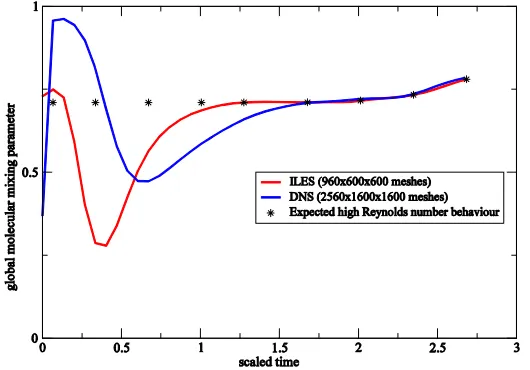
[image:19.595.150.415.503.688.2]The evolution of the global mixing parameter,, is shown in figure 14. The trend is similar to that shown in figures 4 and 10. For the DNS, reaches values close to unity when the initial in-terface diffuses away, then dips to ~0.5 and finally rises to ~0.7. From=1.75 onwards, when the effect of finite Reynolds number is presumed small, values of for ILES and DNS are near-iden-tical. Figure 14 also indicates the expected behavior at very high Reynolds number; a high plat-eau level of~0.7 should quickly be reached andshould increase slightly towards the end of the experiment. The ILES gives an approximation to this behavior at an earlier stage that the DNS. The previous DNS of Livescu showed similar behavior. dipped to a value of ~ 0.47 and the rose to values approaching the ILES results. However, because of the time delay (explained earlier), the previous DNS did not reach the stage where the ILES and DNS results agreed.
The total computer time (processor – hours) for the DNS was a factor 50 greater than that for the ILES. Hence ILES provides the simplest way of estimating the high-Reynolds number behavior. As noted earlier, if the effect of finite Reynolds number is required, DNS is essential.
5. Concluding Remarks
Three dimensional simulation, DNS, ILES and some examples of LES with explicit dissipation models, has made a major contribution to understanding the process of turbulent mixing by Ray-leigh-Taylor instability. The detailed structure of the mixing zone is difficult to obtain from ex-periments, especially at high Atwood number, and 3D simulation is able to fill this gap. However, one important result is learnt from experiments. Typical experiments give~0.06 whereas simu-lations, using a wide range of techniques, with ideal initial conditions (random short wavelength perturbations) give~0.026. A likely explanation of this is the presence of low levels of long wavelength initial perturbations in the experiments. The experimental results show that mixing in real situations will usually be significantly greater than that for the ideal theoretical case.
The main purpose of the paper has been to give a direct comparison of results for DNS and ILES using the same numerical framework. It has been shown here that, provided the mesh resolution is sufficient to resolve fine-scale structure within the mixing zone, ILES and DNS give very simi-lar results. This applies to quantities such as distributions mean volume fractions, molecusimi-lar mix-ing parameter or turbulence kinetic energy. The Navier-Stokes results given here are not fully-converged DNS. However, the deviation from fully-fully-converged DNS has been quantified and it argued that the mainly global results given here are accurate. For quantities such as enstrophy, which are determined by the small scales present in the flow, DNS is required to get meaningful results (probably with higher resolution or with higher order numerics being required to obtain accurate results). DNS may also be needed if more complex physics is present (combustion for example). If the main purpose of the simulations is to obtain the high-Reynolds behavior of global properties, then this can be achieved using ILES with much less computer resources than with DNS. The early stages of the mixing process are influenced by viscosity and diffusivity and DNS is essential for understanding the influence of Reynolds number and Schmidt number on the mixing process.
The DNS results given here have used a relatively simple numerical approach. It is argued that satisfactory results have been obtained for the influence of finite Reynolds number on the mainly global results presented. Further research is needed to assess the suitability of the method for the accurate calculation of fine-scale properties.
and ILES have an essential contribution to make to calibration and validation of such models. At present, DNS results may be used for model calibration/validation in simple situations, such as one-dimensional mixing layers. However, as engineering models need to be applied to much more complex problems, validation is needed for a wide range of benchmarks. It is advocated that comparisons of RANS and ILES have an essential role here.
Acknowlegements
The computational results shown in this paper were generated when the author was employed by AWE, Aldermaston, United Kingdom. The paper contains material © British Crown Owned Cop-yright 2017/AWE.
References
Amendt P, Colvin J D, Tipton R E, Hinkel D E, Edwards M J, Landen O L, Ramshaw J D,
Suter L J, Varnum W S and Watt R G 2002 Indirect-drive noncryogenic double-shell ignition targets for the National Ignition Facility: design and analysisPhysics of Plasmas92221-2233
Abarzhi S I 2010 Review of theoretical modeling approaches of Rayleigh-Taylor instabilities and turbulent mixingPhil. Trans. Roy. Soc. A3681809-1828
Abarzhi S I and Rosner R 2010 A comparative study of approaches for modeling Rayleigh-Taylor turbulent mixingPhys. Scr. T142014012 (13pp)
Andrews M J and Dalziel S B 2010 Small Atwood number Rayleigh–Taylor experimentsPhil. Trans. Roy. Soc. A3681663-1679
Andrews M J, Youngs D L, Livescu D and Wei T 2014 Computational studies of two-dimensional Ray-leigh-Taylor driven mixing for a tilted-rig ASME Journal of Fluids Engineering136091212(14pp) Anuchina N N, Kucherenko Yu A, Neuvazhaev V E, Ogibina V N, Shibarshov L I and Yakovlev V G, 1978 Turbulent mixing at an accelerating interface between liquids of different densityIzv. Akad. Nauk SSSR, Mekh. Zhidk. Gaza6157-160
Belen’kii S Z and Fradkin E S 1965 Theory of turbulent mixingFiz. Inst. Akad. Nauk SSSR29207-238
Banerjee A and Andrews M J 2009 3D Simulations to investigate initial condition effects on the growth of Rayleigh–Taylor mixingInternational Journal of Heat and Mass Transfer523906-3917
Birkhoff G 1954 Taylor instability and laminar mixing Los Alamos report LA-1862
Burton G C 2011 Study of ultrahigh Atwood-number Rayleigh–Taylor mixing dynamics using the nonlin-ear large-eddy simulation methodPhysics of Fluids23045106(16pp)
Cabot W H and Cook A W 2006 Reynolds number effects on Rayleigh-Taylor instability with possible im-plications for type-1a supernovae Nature Phys.2562 -568
Cook A W and Dimotakis P E 2001 Transition stages of Rayleigh–Taylor instability between miscible flu-idsJournal of Fluid Mechanics44369-99
Cook A W and Zhou Y 2002 Energy transfer in Rayleigh-Taylor instabilityPhysical Review E66 026312(12pp)
Cook A W, Cabot W and Miller P L 2004 The mixing transition in Rayleigh–Taylor instabilityJournal of Fluid Mechanics511333-362
Dalziel S B, Linden P F and Youngs D L 1999 Self-similarity and internal structure of turbulence induced by Rayleigh-Taylor instabilityJ. Fluid Mech.3991-48
DeBar R 1974 Fundamentals of the KRAKEN codeLawrence Livermore Laboratory UCIR-760
Denissen N A, Rollin B, Reisner J M and Andrews M J 2014. The tilted rocket rig: a Rayleigh–Taylor test case for RANS modelsJournal of Fluids Engineering136091301
Dimonte G and Schneider M 1996 Turbulent Rayleigh-Taylor instability experiments with variable acceler-ationPhys. Rev. E 543740-3743
Dimonte G and Schneider M 2000 Density ratio dependence of Rayleigh-Taylor mixing for sustained and impulsive accelerations Phys. Fluids12304-321
Dimonte G 2004 Dependence of turbulent Rayleigh-Taylor instability on initial perturbationsPhys. Rev. E
69056305(14pp).
Dimonte G, Ramaprabhu P and Andrews M 2007 Rayleigh-Taylor instability with complex acceleration historyPhysical Review E76046313(6pp)
Dimotakis P E 2000 The mixing transition in turbulent flows J. Fluid Mech.40969-98
Fryxell B, Arnett D and Mueller E 1991 Instabilities and clumping in SN 1987A. I-Early evolution in two dimensionsThe Astrophysical Journal367619-634
Glimm J, Grove J W, Li X L, Oh W and Sharp D H 2001 A critical analysis of Rayleigh–Taylor growth ratesJournal of Computational Physics169652-677
Glimm J, Sharp D H, Kaman T and Lim H 2013 New directions for Rayleigh–Taylor mixingPhil. Trans. R. Soc. A37120120183(17pp)
Grinstein F F, Margolin L G and Rider W J (eds) 2007Implicit Large Eddy Simulation: computing turbu-lent flow dynamicsNew York: Cambridge University Press
Inogamov N A 1978 Turbulent stage of the Rayleigh–Taylor instabilitySov. Tech. Phys. Lett.4299-304
Kokkinakis I W, Drikakis D, Youngs D L and Williams R J R 2015 Two-equation and multi-fluid turbu-lence models for Rayleigh–Taylor mixingInternational Journal of Heat and Fluid Flow56233-250 Kull H J 1991 Theory of the Rayleigh-Taylor instabilityPhysics Reports206197-325
Lawrie A G W and Dalziel S B 2011 Turbulent diffusion in tall tubes. I. Models for Rayleigh-Taylor insta-bilityPhysics of Fluids23085109(9pp)
Linden P F, Redondo J M and Youngs D L 1994 Molecular mixing in Rayleigh–Taylor instabilityJournal of Fluid Mechanics26597-124
Livescu D, Ristorcelli J R, Petersen M R and Gore R A 2010 New phenomena in variable-density Ray-leigh–Taylor turbulencePhysica ScriptaT142014015(11pp)
Livescu D, Wei T and Petersen M R 2011 Direct numerical simulations of Rayleigh-Taylor instability
Journal of Physics: Conference Series318082007(10pp)
Livescu D 2013 Numerical simulations of two-fluid turbulent mixing at large density ratios and applica-tions to the Rayleigh–Taylor instabilityPhil. Trans. Roy. Soc. A37120120185(23pp)
Lombardini M, Hill D J, Pullin D I and Meiron D I 2011. Atwood ratio dependence of Richtmyer–Mesh-kov flows under reshock conditions using large-eddy simulations.Journal of fluid mechanics670439-480. Mueschke N J and Schilling O 2009a Investigation of Rayleigh–Taylor turbulence and mixing using direct numerical simulation with experimentally measured initial conditions. I. Comparison to experimental data
Physics of Fluids21014106(19pp)
Mueschke N J and Schilling O 2009b Investigation of Rayleigh–Taylor turbulence and mixing using direct numerical simulation with experimentally measured initial conditions. II. Dynamics of transitional flow and mixing statisticsPhysics of Fluids21014107(16pp)
Mueschke N J, Schilling O, Youngs D L and Andrews M J 2009 Measurements of molecular mixing in a high-Schmidt-number Rayleigh-Taylor mixing layer J. Fluid Mech.63217-48
Olson B J, Larsson J, Lele S K and Cook A W 2011 Nonlinear effects in the combined Rayleigh-Tay-lor/Kelvin-Helmholtz instabilityPhysics of Fluids23114107(10pp)
Ramaprabhu P and Andrews M J 2004 On the initialization of Rayleigh–Taylor simulationsPhysics of Flu-ids 16L59-L62
Ramaprabhu P, Dimonte G and Andrews M J 2005 A numerical study of the influence of initial perturba-tions on the turbulent Rayleigh–Taylor instabilityJournal of Fluid Mechanics536285-319
Ramaprabhu P, Karkhanis V and Lawrie A G W 2013 The Rayleigh-Taylor Instability driven by an accel-decel-accel profilePhysics of Fluids25115104(33pp)
Read K I 1984 Experimental investigation of turbulent mixing by Rayleigh-Taylor instabilityPhysica D12 45-58
Rehagen T J, Greenough J A and Olson B (2017) A validation study of the compressible Rayleigh-Taylor instability comparing the Ares and Miranda codes.Journal of Fluids Engineering(accepted)
Ristorcelli J R and Clark T T 2004 Rayleigh–Taylor turbulence: self-similar analysis and direct numerical simulationsJ. Fluid Mech.507213-253
Schilling O and Mueschke N J 2010 Analysis of turbulent transport and mixing in transitional Rayleigh– Taylor unstable flow using direct numerical simulation dataPhysics of Fluids22105102(26pp)
Sharp D H and Wheeler J A 1961 Late stage of Rayleigh-Taylor instabilityDefense Technical Information Center (DTIC) document ADA009943
Sharp D H 1984 An overview of Rayleigh-Taylor instabilityPhysica D123-18.
Sreenivasan K R, Gauthier S and Abarzhi S I (eds) 2013 Turbulent mixing and beyond: non-equilibrium processes from atomistic to astrophysical scales IIPhil. Trans. Roy. Soc. London A371
Statsenko V P, Yanilkin Yu V and Zhmaylo V A 2013 Direct numerical simulation of turbulent mixing.
Phil. Trans. Roy. Soc. London A37120120216(19pp)
Tsoutsanis P, Kokkinakis I W, Könözsy L, Drikakis D, Williams R J R and Youngs D L 2015 Comparison of structured-and unstructured-grid, compressible and incompressible methods using the vortex pairing problem.Computer Methods in Applied Mechanics and Engineering 293207-231
Van Leer B 1977 Towards the ultimate conservative difference scheme. IV. A new approach to numerical convectionJournal of computational physics23276-299
Williams R. J. R. 2017. Rayleigh–Taylor mixing between density stratified layers.J. of Fluid Mechanics, 810, 584-602
Young Y-N, Tufo H, Dubey A and Rosner R, 2001 On the miscible Rayleigh–Taylor instability: two and three dimensionsJournal of Fluid Mechanics447377-408
Youngs D L 1989 Modelling Turbulent Mixing by Rayleigh-Taylor InstabilityPhysica D37270-287
Youngs D L 1991 Three‐dimensional numerical simulation of turbulent mixing by Rayleigh–Taylor
insta-bilityPhysics of Fluids A31312-1320
Youngs D L 1994 Numerical simulation of mixing by Rayleigh-Taylor and Richtmyer-Meshkov instabili-tiesLaser and Particle Beams12725-750
Youngs D L 2003 Application of MILES to Rayleigh-Taylor and Richtmyer-Meshkov mixingAIAA paper 2103-4102
Youngs D L 2007 The Lagrangian Remap MethodImplicit Large Eddy Simulation: Computing Turbulent Fluid Dynamics (chapter 4c)New York: Cambridge University Press
Youngs D L 2009 Application of monotone integrated large eddy simulation to Rayleigh–Taylor mixing Phil. Trans. Roy. Soc. A3672971-2983
Youngs D L 2013 The density ratio dependence of self-similar Rayleigh–Taylor mixingPhil. Trans. Roy. Soc. A37120120173(15pp)