Math expression retrieval using symbol pairs in layout trees

Rochester Institute of Technology

RIT Scholar Works

Theses Thesis/Dissertation Collections

8-1-2013

Math expression retrieval using symbol pairs in

layout trees

David Stalnaker

Follow this and additional works at:http://scholarworks.rit.edu/theses

Recommended Citation

Math Expression Retrieval Using

Symbol Pairs in Layout Trees

by

David Stalnaker, B.S.

THESIS

Presented to the Department of Computer Science

Golisano College of Computer and Information Sciences

in Partial Fulfillment

of the Requirements

for the Degree of

Master of Science

Math Expression Retrieval Using

Symbol Pairs in Layout Trees

APPROVED BY

SUPERVISING COMMITTEE:

Dr. Richard Zanibbi, Chair

Dr. Bo Yuan, Reader

Math Expression Retrieval Using

Symbol Pairs in Layout Trees

David Stalnaker, M.S.

Rochester Institute of Technology, 2013

Advisor: Dr. Richard Zanibbi

We have developed a layout-based math retrieval system by indexing on

pairs of symbols in mathematical expressions. Existing approaches to

layout-based retrieval include tree edit distance-layout-based matching on MathML trees

(Kamali and Tompa, 2013) and longest common subsequence matching in

LA_{TEX strings (Kumar et al., 2012). In our work, we compare our new}

layout-based retrieval method with a math retrieval system built using the

conven-tional text-based retrieval system Lucene (Zanibbi and Yuan, 2011), as such

systems are commonly used for math search. We show that the search results

returned by our system are scored by participants in a study as significantly

more similar than those of the comparison system and that our system is fast

Table of Contents

Abstract iii

List of Tables vi

List of Figures vii

Chapter 1. Introduction 1

Chapter 2. Background 4

2.1 Information Retrieval . . . 4

2.2 Index Compression . . . 5

2.3 Math Retrieval . . . 7

2.4 Ranking Math Query Results . . . 11

2.5 MathML . . . 12

2.6 Summary . . . 14

Chapter 3. Methodology 15 3.1 Corpora . . . 15

3.1.1 MREC . . . 15

3.1.2 Wikipedia . . . 16

3.2 Input Formats . . . 16

3.3 Symbol Layout Trees . . . 17

3.4 Symbol Pairs . . . 18

3.5 Symbol Pair Index . . . 19

3.6 Ranking Functions . . . 21

3.7 Implementation . . . 26

Chapter 4. Results and Discussion 29

4.1 Experimental Design . . . 29

4.1.1 Query Result Relevance . . . 29

4.1.2 System Performance . . . 32

4.2 Results . . . 33

4.2.1 Demographics and Survey Responses . . . 33

4.2.2 Search Result Scores . . . 33

4.2.3 Response Times . . . 37

4.3 Performance Metrics . . . 38

4.4 Discussion . . . 39

4.5 Summary . . . 41

Chapter 5. Future Work and Conclusion 42 5.1 Future Work . . . 42

5.1.1 Performance Optimizations . . . 42

5.1.2 Retrieval Improvements . . . 43

5.1.3 Additional Comparisons . . . 45

5.2 Conclusion . . . 46

Appendices 47

List of Tables

3.1 Definitions for the ranking functions . . . 22 3.2 Important Redis keys and their values. . . 27

List of Figures

1.1 Screenshots of min and Tangent . . . 2

2.1 Size of encoded values . . . 7

3.1 Example expression, Symbol Layout Tree, and Symbol Pairs . 18 3.2 Pseudocode for indexing and searching. . . 20 3.3 Example query and result for Prefix ranker . . . 25 3.4 Pseudocode for the Prefix ranking function. . . 26

Chapter 1

Introduction

While search for text is a well-studied problem, math search is less

ma-ture. Search for mathematical expressions is difficult for a number of reasons.

There are numerous representations for expressions, including: LA_TEX,

(con-tent and presentation) MathML, Mathematica, and various forms of rendered

output (PDF, images). Mathematical expressions are generally expressed as

a tree structure (whereas text is linear), which necessitates more complex

al-gorithms for matching. Partially matched expressions are difficult to rank

because small syntactic changes can have large semantic meaning and vice

versa.

The main motivation for a math search engine is to facilitate learning.

Upon coming upon an unfamiliar mathematical expression, a student could

search for it and learn what it means. Similarly, a researcher could find

pa-pers by searching the math contained within them [17]. Math search could

also be used when mathematical queries are detected in an existing search

en-gine [2]. One problem with a math search enen-gine is that the representations of

mathematics are complex and students are unlikely to be familiar with them.

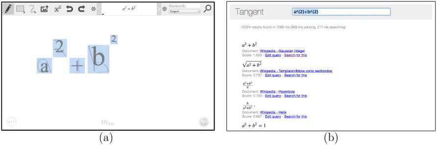
hand-written mathematics and can be used as an input for our search engine.

Figure 1.1 shows the interaction between these two systems.

(a) (b)

Figure 1.1: Screenshots of the min handwritten math recognition tool

(a), and the results page of our Tangent search engine (b).

An inverted index is the tool used most commonly in text search. It is

a lookup table from words to the documents that contain them. This idea has

been modified to allow for word locality, phrase searching, index compression,

and distributed indexing. With these and other improvements, systems can

be built to quickly search massive corpora (notably the Internet) [20].

In our system, Tangent, we apply the concept of the inverted index to

math search, indexing directly on the structure of the equation instead of a

linear string representation thereof. The idea is that encoding the structure of

the expression directly in the index will yield more partial matches, providing

text search, overall system speed should be comparable to those systems. This

leads us to this hypothesis:

Implementing a math expression search system using an

inverted index on symbol pairs from layout trees will: 1)

yield more relevant results than text-based retrieval, and

2) be fast enough for real time use.

We conducted two experiments to test our hypothesis: a human study

wherein we asked participants to score results from our system and a text

search-based comparison system, and a performance analysis of our system.

The results of these experiments support both parts of the hypothesis. The

search results for our system scored significantly higher than those of the

com-parison system and a performance analysis showed the system to be usable

Chapter 2

Background

Information retrieval is a well-established field in computer science, but

the majority of the research has been focused on text retrieval with significantly

less work in math retrieval. In this chapter, we will describe the basic concepts

used in text retrieval, and methods to compress the indexes used therein.

We will then describe several existing math search systems and discuss the

general goals of math retrieval. Finally, we will describe MathML, a common

representation for mathematical expressions.

2.1

Information Retrieval

As computers appeared, one of the important tasks that emerged was

storing and searching large sets of documents. The inverted index was an

early and natural development in this field. It can be thought of like an index

in a book: it is a structure that maps each term to a list of documents that

contains it. In its most simple form, an inverted index only allows us to find

the documents that contain a given term [7, 10].

The inverted index is still the basis of almost every document retrieval

powerful. By looking up multiple terms and taking the union or intersection of

the returned set of documents, we can handle multi-term queries. By storing

the frequencies of terms in each document, we can order the documents by

this frequency. By storing the location(s) of each term in each document, we

can search for exact and inexact phrases.

There are numerous ways in which to rank the relevance of matched

documents. The simplest is the frequency of a matched term in the

docu-ment, or term frequency. A common metric, TF-IDF, makes use of this and

the Inverse Document Frequency. The IDF is the inverse of the number of

documents that contain the term. Including this in a ranking metric allows

us to bias results towards infrequently used words, which works well because

common words are usually less discriminative. Other measures that might be

used as part of a ranking metric are the number of documents and terms in

the index, and the term frequency.

2.2

Index Compression

While storing document references and counts in the index as 32- or

64-bit integers is convenient, it is wasteful of space. There are numerous

ways to compress the inverted lists. In addition to the decreased storage

need, this also usually brings a performance improvement, as the added cost

of decompression is negligible compared to the decreased cost of disk reads.

Most of the compression methods discussed will remain applicable with the

is a summary of Zobel and Moffat’s discussion of the same topic in [20].

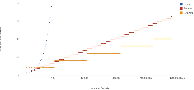
One way to compress an index is to change the representation of an

integer. The appropriate representation depends on the probability

distribu-tion of the values. If the values are very low, a unary representadistribu-tion is viable,

wherein the numbernis is represented by n−1 “1” bits followed by a “0” bit.

This has the property that “1” is encoded with just 1 bit, but quickly becomes

inefficient for larger values. Unary encoding is most efficient when P[n]≈ 1 2n,

where n is the number being encoded and P is the probability distribution of

the numbers to be encoded. In practice this means n must be very small.

Elias’ gamma code allows for more efficient encoding of larger numbers.

The value n is factored into 2e_{+d, where e=blog}

2nc. The encoding is then

e+ 1 encoded in unary followed by d encoded in binary (using e bits). It is

most efficient when P[n]≈ 1 2n2.

While bitwise encoding schemes can lead to a great reduction in index

size, they ignore the fact that computers can generally only address memory

at the byte level. It is thus often a better idea to encode our index in whole

bytes, for reason of both performance and ease of programming. An effective

method is to break the value into 7-bit chunks. If the value fits in 7 bits,

encode it in one byte with the high bit set to “0”. Otherwise, encode the

first 7 bits with a leading “1”, and iterate with the next byte. This is more

wasteful than the bitwise methods for small values, but in practice provides a

Figure 2.1: Size of encoded values. Input values are on a log scale, and the unary encoding is far off the scale for large values.

These encoding schemes work well for frequency counts because they

are generally very small. Document IDs, however, are distributed uniformly

and thus do not compress well. An effective way to solve this is to sort the

document identifiers in each inverted list and store instead the differences

between each element and its predecessor. In a list for a common word (which

will make up a sizable portion of the index), these differences will be very

small and compress easily.

2.3

Math Retrieval

There are several systems for math search that encode expressions as

key effort here is the process of “linearizing” the math expression for input

into the text search system, both for documents to index and queries to the

system. Zanibbi and Yuan’s system [19] indexes individual LA_{TEX expressions}

by tokenizing the expression and mapping each symbol to a text

represen-tation. In this example from Miller [8], the LA_{TEX expression x^{t-2} = 1}

is represented as x BeginExponent t minus 2 EndExponent Equal 1. Ex-pressions are then inserted into the Lucene search engine and queried with

LA_{TEX expressions processed in the same manner.}

Sojka and L´ıˇska’s MIaS system [14, 15] operates on similar principles

but differs in several areas. It is a full-text search system that indexes both

math expressions and the surrounding text. Instead of single LA_TEX

expres-sions, MIaS indexes XHTML documents containing MathML expressions. The

overall architecture of the system is similar, with linearized expressions being

inserted into a text search system (it too uses Lucene). Munavalli and Miner’s

MathFind [9] is another text-search based system, indexing text and MathML

expressions together by converting the expressions to text strings.

The key problem with this approach is that the text search has limited

information on the structure of the expression. It is thus difficult to align

the qualities of a good textual match with the qualities of a good match of

the expression. The advantages are that it works reasonably well in practice,

is easy to implement, and benefits directly from the decades of research in

document retrieval. Our approach will use the same concept of the inverted

expressions.

There have been several approaches which look at the problem more

directly. Kamali and Tompa describe a system based on efficient exact

match-ing of MathML trees [3]. They use an index in which identical subtrees are

shared between all expressions, which allows for much better performance.

In-exact matching is enabled through the use of wildcards, where each wildcard

can be a number, variable, operator, or expression (which can itself contain

wildcards). More recently, they describe a system that uses a similar index

but uses a tree-edit distance for searching and ranking, which allows for

in-exact matching without user-specified wildcards [4]. Calculating the tree-edit

distance for each expression in the index would be too expensive, but through

a combination of early termination for poor matches and caching for

subex-pressions, it achieves competitive performance (∼_{800ms query time on a large}

corpus compared to ∼_{300ms for MIaS).}

Kumar et al. [6] use a Least Common Subsequence (LCS) algorithm for

matching LA_{TEX strings. The input L}A_{TEX strings are preprocessed as a}

canon-icalization step where each function, variable, and number is mapped to an

atomic term. Variables and numbers are generalized. A dynamic-programming

LCS algorithm on these terms is then used to find the matches. This approach

is fairly robust against small changes in the structure (i.e. it allows for inexact

matching) as missing or modified parts of the expression will be gaps in the

LCS. However the LCS algorithm is O(n2_{) in the expression size and requires}

for large indexes.

Another approach to the problem uses substitution trees. Substitution

trees come from the field of automatic theorem proving. The leaf nodes contain

the expressions that have been inserted into the tree. The internal nodes

contain expressions with at least one generic term. Each child represents a

substitution of one or more of the generic terms of its parent with more specific

terms (which can introduce new generic terms).

Kohlhase and Sucan’s Math WebSearch [5] uses substitution trees to

match expressions on their semantic meaning, rather than layout. This

ap-proach can match expressions that match the query term exactly up to α

-equivalence, which means the structure must match exactly but individual

terms may be substituted (to terms of the same type). In addition,

subex-pression matching was enabled by inserting all subexsubex-pressions of an

expres-sion when inserting it into the index. Input to Math WebSearch is Content

MathML (see Section 2.5).

Schellenberg’s work [12, 13] instead uses substitution trees to match

ex-pressions by their layout. Rather than performing an exact expression match

(as Math WebSearch does), this system exhaustively searches the tree for

matches. This has the benefit of allowing for partial matches that have

struc-tural similarity, but the drawback of greatly increased query times. The system

introduces a ranking method for partial matches which will be discussed in the

2.4

Ranking Math Query Results

While very effective metrics have been developed for ranking text queries,

ranking math expressions remains an open question. There are some analogs

between the two problems (for example, the concept of term frequency can

be roughly applied in the same way to symbols in an expression), but a new

strategy is needed.

Mathematical expressions can generally be considered to have a tree

structure, unlike text which is linear. As such, the structure of the expression

is important to capture in the ranking metric. Symbols in an expression can

easily be broken into categories: operators, variables, constants, and functions.

These categories should have different weights in the ranking function (e.g.

operators have more meaning than variables, which can be renamed without

much change to the expression) [16]. Relatedly, a useful quality for a ranking

function to have would be to match expressions with the identical structure

but variables renamed, with a penalty.

Another positive quality for a ranking function would be to favor results

in which the matched symbols are more connected to each other than not. A

common type of query would be one that matches a small part of a larger

expression. For example, take the queryx+y. The result (x+y)∗zwould be a

better match than (x+z)∗y, because the query term is an exact subexpression.

According to this quality, the more relevant result would thus be the one that

While most systems rely on their underlying text search systems for

ranking partial matches, there have been some attempts made at ranking

math expressions directly. Schellenberg [12, 13] defines a ranking function that

combines two metrics: a bag-of-words comparison of the individual symbols

in the expressions and a bipartite comparison that looks at pairs of symbols

(including the structure between them: the relationship between the symbols

and position along the baseline). For each of these metrics, the number of

matching symbols / pairs is counted, and the average of these two scores is

taken. Additionally, symbols that match the correct type but not the exact

symbol are counted at 25% of a full match. While our index will be built using

a different method than that of this system, our ranking function will build

directly on its ideas.

2.5

MathML

MathML is an XML-based language for describing mathematical

ex-pressions. There are two forms: Content MathML describes semantic

mean-ing and Presentation MathML describes layout. While some systems (Math

WebSearch [5]) build indexes on semantics, we will be focusing on layout and

thus Presentation MathML.

A MathML expression is contained in a root <math> tag. There are

four token elements (elements that do not contain other elements): identifiers

(<mi> ), operators ( <mo> ), numbers ( <mn> ), and text ( <mtext> ).

of adjacent elements. Each of the child elements are placed in a row. The

<mfrac> tag describes a fraction. The first child is the numerator and the

second is the denominator. The <msup> tag describes a superscript, with the

first child being the base and the second being the exponent. <msub> and

<msubsup> tags describe subscripts and combination subscript-superscripts,

respectively. Similarly, <mover> , <munder> , and <munderover> describe

elements that are directly under and/or over an element (e.g. an integral

sign). The <msqrt> tag describes the square root of its only child and the

<mroot> tag describes the n-th root of its first child, where n is its second

child. Tables are contained in <mtable> elements and contain rows ( <mtr>

) which contain cells ( <mtd> ). The <mfenced> tag describes a group where

its children are surrounded by some fence symbol (e.g. parentheses).

As Presentation MathML can represent the same expression in multiple

ways, a canonicalization procedure is needed to prevent a valid match from

being ignored because it was represented differently. Archambault and Mo¸co

define Canonical MathML [1], an extension of Presentation MathML that

does exactly this. Canonicalization is important because we are encoding the

structure obtained from the MathML in our index. If an expression can take

multiple forms in our index, a matching query and result could appear to

not match if they are expressed differently in MathML, even when they are

describing the same expression.

In Canonical MathML, all tags like <msub> , <mfrac> , and <mroot>

enforcing the use of the <mrow> tag where it is not strictly necessary in

standard MathML. Summation, product, and integrals must be contained in a

two-element row. The first element is the symbol, which might also be wrapped

in a <msub> or <msubsup> tag. The second element is the subexpression

being (for example) summed, which must be wrapped in a second <mrow> if

it contains multiple symbols. Similarly, a parenthesis group is contained in a

<mrow>, with all fence symbols and commas as <mo> elements in it.

A common and more human-readable representation of mathematical

expressions than MathML is LA_{TEX. L}A_{TEX expressions are presentational and}

can be converted to Presentation MathML (see Section 3.1).

2.6

Summary

Existing methods of math information retrieval can be generally broken

up into two groups: adaptations of existing text search tools or some form of

tree-matching. The approach we describe in the next section takes a different

tack: we apply the idea of an inverted index more directly on the structure of

Chapter 3

Methodology

Tangent uses an inverted index of pairs of symbols from expressions.

In this chapter, we will describe the corpora and formats used for math

repre-sentation. We will define the Symbol Layout Trees and the Symbol Pairs used

in the index, and then the index itself. Then, we will define 5 different ranking

functions for ordering matches. Finally, we will describe the implementation

of our system.

3.1

Corpora

3.1.1 MREC

MREC (Math REtrieval Collection) is a collection of approximately

324,000 academic publications. The arXiv1 _{contains preprint papers in}

sci-ence and mathematics. These documents have been converted to XHTML

and MathML by the LaTeXML2 _{project. MREC takes the documents that}

have been converted successfully and modifies them, most importantly by

con-verting the MathML expressions to Canonical MathML.

1_{http://arxiv.org}

3.1.2 Wikipedia

The Wikipedia corpus contains every mathematical expression from

the English-language Wikipedia project. It contains mathematical expressions

from virtually every field and more importantly, definitions and explanations

thereof. It is a desirable corpus because the information it contains is helpful

in learning mathematics, which is one of the major use cases of a math search

system. Additionally, we feel it is ideal for a comparison between search engines

because the breadth rather than depth of the mathematics represented. Each

concept might only have a few expressions, but with so many articles covering

so much material, it is likely that a given query will have a wide variety of

relevant results.

The corpus was assembled from a full XML archive of English Wikipedia

created on May 4, 2013. The LaTeX expressions were extracted from the

doc-ument along with the associated articles. The extracted LaTeX expressions

were then converted into MathML documents using the same LaTeXML tool

as used by MREC. There are 482,364 expressions contained in 32,780 articles.

3.2

Input Formats

Our system can parse both LA_{TEX expressions and the XHTML +}

Canonical MathML files from the MREC and Wikipedia datasets. For

sim-plicity, we use LaTeXML (the same tool used to create the datasets) to convert

any LA_{TEX expressions to MathML, which we then parse into Symbol Layout}

ex-pressions are also necessary as MathML is too unwieldy for user input (for the

query expression). In practice, the index will likely be built from MathML and

search queries will be input with LA_{TEX (either written by the user or generated}

by our handwritten math recognition tool, min [11]). Every commonly-used

MathML tag (all of those found in both corpora) is supported with the

excep-tion of those related to tables. The Symbol Pair representaexcep-tion used for the

index is not well-defined for tables, so MathML expressions containing tables

are ignored.

3.3

Symbol Layout Trees

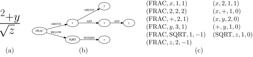
Internally, Tangent uses a Symbol Layout Tree (SLT) to represent

ex-pressions. The vertices in this tree are the symbols in the expression and the

edges are the spacial relationships between them. The tree is rooted at the

leftmost symbol on the main baseline. Each symbol can have a relationship

to those ABOVE, BELOW, ADJACENT to, and WITHIN it. Examples of

ABOVE relationships include superscripts and upper limits on integrals (in

some SLT representations these would be separate relationships, but we have

combined them). Similarly, BELOW relationships include subscripts and lower

limits. Fractions are encoded as a FRAC symbol with the numerator ABOVE

and the denominator BELOW. A square root can have an expression WITHIN

it, and most other symbols will be ADJACENT (always to the right).

Fig-ure 3.1 shows an example expression, its Symbol Layout Tree, and its Symbol

x

√

2

+

y

z

x ABOVE

SQRT BELOW

2 ABOVE

+ ADJ

z WITHIN

y ADJ

(FRAC, x,1,1) (x,2,1,1) (FRAC,2,2,2) (x,+,1,0) (FRAC,+,2,1) (x, y,2,0) (FRAC, y,3,1) (+, y,1,0) (FRAC,SQRT,1,−1) (SQRT, z,1,0) (FRAC, z,2,−1)

(a) (b) (c)

Figure 3.1: Example expression (a), Symbol Layout Tree (b), and Sym-bol Pairs(c)

3.4

Symbol Pairs

In text information retrieval, the documents are split into words to be

inserted into an index. To (naively) apply this idea directly to mathematics,

we could insert each symbol from an expression into the index, but this would

lose all information about the structure of the expression.

Our approach is to instead add pairs of symbols to the index. The

pairs are encoded with a representation of the structure between them. This

Symbol Pair representation is a tuple (s1, s2, dh, dv) where s1 and s2 are the

two symbols in the pair. The horizontal distance, dh, is the length of the

path between s1 and s2 when traversing the SLT. It can also be thought of

the number of symbols between s1 and s2 when moving rightward along the

baseline (though not strictly true as, for example, the ABOVE relationship

between a FRAC and a numerator counts towardsdh but does not move

right-ward). The vertical distance, dv, is the height of s2 aboves1’s baseline, which

is not affected by ADJACENT or WITHIN relationships. For example, in

the expression xy _{+z, we would add (x, y,1,1), (x,+,1,0), (x, z,2,0), and}

(+, z,1,0) to the index. This representation is chosen to maintain the relative

relationship between the pair of symbols but be general enough to be used for

partial matches.

The Symbol Pairs are generated between every symbol (s1) in the SLT

and every symbol in the subtrees (children) of s1. This means that s1 is

always a parent element of s2 in the SLT. Not all pairs of symbols from the

SLT will be included; specifically, two symbols that in separate child subtrees

of a parent will not be included when generating the Symbol Pairs for an

expression. There are a worst-case n₂ pairs inserted for an expression with n

symbols, which would occur for any linear expression (i.e. when there are no

branches in the SLT).

3.5

Symbol Pair Index

The index we have developed is similar to that of a text search engine,

with Symbol Pairs instead of words. The index is a hash table mapping Symbol

Pairs to the list of expressions that contain them. To create the index, we look

up each symbol pair in the index (creating an empty list if none was found)

and append the expression to the list that was found.

Querying the index is more complex. We construct a hash table,

re-sult pairs, that maps each matching expression to a list of the Symbol Pairs

the query expression in the index, getting a list of expressions that contain

that pair. Then, for each expression in that list, we add the pair to the

re-sult pairs entry for that expression. The full list of rere-sult expressions are then

ordered by a ranking function, which is given the search expression, the result

expressions, and the list of matching Symbol Pairs for each result expression.

It is possible for an expression to contain the same Symbol Pair more

than once. When this happens, we count the pair n times, where n is the

minimum of number of times the pair occurs in the query and the result. For

example, if a Symbol Pair occurs 5 times in a result but only twice in the

query, we will count it twice.

Index(expression, index):

for pair in symbol pairs of expression: append expression to index[pair] Search(query, index, k):

for pair in symbol pairs of query: for expression in index[pair]:

append pair to result_pairs[expression]

sort expressions by the ranking function (using result_pairs) return the top k expressions

Figure 3.2: Pseudocode for indexing and searching.

In text search, the index often includes in the lists the position in the

document where each word was found. Analogously, we include an identifier

that defines the absolute position of s2. This identifier is a d-element list,

a 0, 1, 2, or 3 depending on whether the ith relationship in the path to s2 is

BELOW, ABOVE, ADJACENT, or WITHIN, respectively. Because dh tells

us the path length betweens1ands2, we can later calculate the identifier fors1

by removing the last dh elements of s2’s identifier. As only one of the ranking

functions uses this information, we have not included it in the pseudocode for

clarity.

3.6

Ranking Functions

It is necessary to apply a ranking function to rank the matched

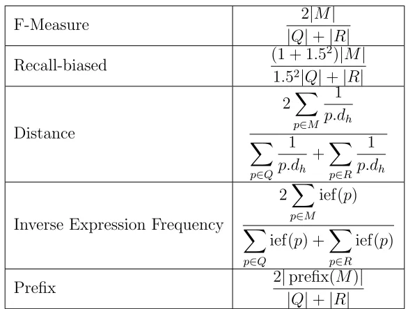
expres-sions by some metric of relevance. We have developed several such functions:

F-Measure, Recall-Biased, Distance, Prefix, and Inverse Expression Frequency.

F-Measure is the baseline, which balances between recall and precision of the

match. The rest of the the ranking functions are each a modification to the

F-Measure, usually by weighting each pair somehow. Recall-Biased uses a

weighted F-Measure to prefer matches that contain most of the Symbol Pairs

in the query. Distance gives higher weight to the Symbol Pairs that are closer.

Inverse Expression Frequency gives higher weight to the Symbol Pairs that are

less common in the index. Prefix removes Symbol Pairs that are from different

parts of the query.

F-Measure Ranker. Our baseline metric is the F-Measure ranker.

The recall-of-match is the percentage of Symbol Pairs in the query that are in

the match, and the precision-of-match is likewise the percentage matched in

F-Measure 2|M|

|Q|+|R|

Recall-biased (1 + 1.5

2_)|M|

1.52_|Q|+|R|

Distance

2X

p∈M

1 p.dh

X

p∈Q

1 p.dh

+X

p∈R

1 p.dh

Inverse Expression Frequency

2X

p∈M

ief(p)

X

p∈Q

ief(p) +X

p∈R

ief(p)

Prefix 2|prefix(M)|

|Q|+|R|

Table 3.1: Definitions for the ranking functions. Q, R, and M are the sets of Symbol Pairs in the query, result candidate, and match (in-tersection) of the query and result, respectively. Note that each is an F-Measure that has been modified in some way.

the match: _|Q2_||₊M_|R|_|, where Q, R, and M are the sets of pairs in the query, result candidate, and match (between the query and result) respectively. Ranking

just by recall would bias results towards those that have the most pairs in

common with the query, but it is not effective. It would not consider the

length of the result and thus can rank highly results that are very long and

thus have a low percentage (but high number) of matched pairs. In a similar

way, ranking just by precision allows matches that are very short, which is

also undesirable. Using the harmonic mean of these values allows us to strike

an appropriate balance between these two extremes.

modifi-cation to the F-Measure ranker which biases the results slightly towards those

with high recall rather than precision. The reasoning behind this is that that

a user might prefer partial matches that contain the query to those that are

contained in the query. This would bias the system to including results that

contain the query as a subexpression than vice versa. It is more likely that the

user neglected to input part of the expression than he or she input too much.

The formula for the Recall-Biased ranker is the F1.5 score, where the general

Fβ score is (1 +β2)· precision

·recall (β2_{·precision)+recall}.

Distance Ranker. The Distance ranker gives higher weights to the

pairs whose symbols are closer. Each pair is weighted by 1/dh, which has the

effect of giving more importance to the pairs that are closer together. The

ranker modifies the F-Measure thusly: instead of counting the set of pairs in

each of M, Q, and R, we sum this 1/dh weight for each Symbol Pair in the

set. The formula for the ranker is then

2X

p∈M

1 p.dh

X

p∈Q

1 p.dh

+X

p∈R

1 p.dh

, where p.dh is the

dh value for p.

Inverse Expression Frequency Ranker. The Inverse Expression

Frequency (IEF) ranker adapts the common text search metric of TF-IDF

(term frequency - inverse document frequency) to the math domain. The

formula ends up being quite different (to that of text search), but the basic

idea is the same: apply more weight to uncommon pairs (terms). We use

match, we sum the inverse expression frequency (IEF) of each matched pair.

The final score is

2X

p∈M

ief(p)

X

p∈Q

ief(p) +X

p∈R

ief(p) .

Prefix Ranker. The Prefix ranker looks at a way to find an alignment

between the query and result expressions and only include pairs in the match if

they occur on that alignment. To provide this alignment we use the additional

path information associated with each pair in the index (See Section 3.5).

Specifically, for each pair in the match, we get the path to s1 in both the

query and the result. These paths are then used to find which pairs share a

common prefix in the match using the algorithm described in Figure 3.4. The

idea is to find the first place (from the symbol moving up the SLT) where the

paths from the query and result diverge. We can then say that the Symbol

Pair is rooted at this this prefix of the two paths. The Symbol Pairs for a

large subexpression match will all be rooted at the same prefix, but Symbol

Pairs that are in different places between the query and result will not - the

idea is to prefer the more connected match.

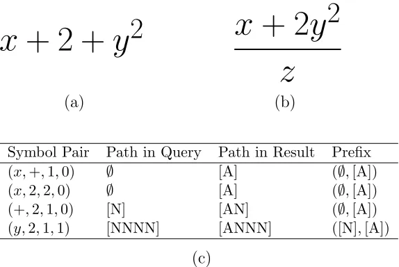
Consider the example query and result in Figure 3.3. Between the

two expressions, there are four matching Symbol Pairs: (x,+,1,0), (x,2,2,0),

(+,2,1,0), and (y,2,1,1). The path to x is ∅ in the query (it is the first

symbol on the main baseline) and [A] in the result (above the FRAC symbol).

The path to + is [N] in the query (one symbol along the baseline) and [AN] in

the result. The path to y is [NNNN] in the query and [ANNN] in the result.

x

+ 2 +

y

2

x

+ 2

y

2

z

(a) (b)

Symbol Pair Path in Query Path in Result Prefix (x,+,1,0) ∅ [A] (∅,[A]) (x,2,2,0) ∅ [A] (∅,[A]) (+,2,1,0) [N] [AN] (∅,[A]) (y,2,1,1) [NNNN] [ANNN] ([N],[A])

(c)

Figure 3.3: Example query (a), result (b), and matched Symbol Pairs and the paths to s1 (c). “A” stands for ABOVE and “N” stands for ADJACENT (next to).

element of the paths differs. For (+,2,1,0), we remove the common N from

the end of the two paths, and get the same prefix of (∅,[A]). For (y,2,1,1),

we can remove three N relationships, but this leaves us with a different prefix

([N],[A]). As 3 matched pairs have the same prefix, this gives us a score of

2∗3

15+16 ≈0.194, whereas the F-Measure would have been

2∗4

15+16 ≈0.258.

The Prefix ranker handles the case of the same pair matching multiple

times differently than the other rankers. We calculate the prefix for all

com-binations of the matches. For example, if a pair was in the query twice and

a result candidate three times, we would calculate the prefix for all 6

PrefixRank(pairs, query_size, result_size): prefixes := dictionary()

for each pair p, with path l_q in the query and l_r in the result: n := max(len(l_q), len(l_r))

pad l_q and l_r with null elements at beginning to length n while last(l_q) == last(l_r):

popright(l_q) popright(l_r)

prefixes[(l_q, l_r)] += 1 largest := max(prefixes)

return f-measure(largest, query_size, result_size)

Figure 3.4: Pseudocode for the Prefix ranking function.

result) of the prefixes can be the same, so this property is maintained from

the other rankers while allowing the prefixes that are in the largest group to

contribute to the result.

3.7

Implementation

The implementation of our system is designed around the Redis3

key-value store. Redis is a robust, scalable, in-memory database that maps string

keys to strings, lists, sets, sorted sets, and hash tables (all of strings). It was

chosen to ease development (as the Tangent server can be restarted

indepen-dently of Redis) and for its high performance. The index and all supporting

information is stored in Redis. As Redis is a simple key-value store, each type

of information is given a key; Table 3.2 lists the most important keys and the

values they store.

Key Value

expr count total # of expressions; next expression id pair:[sp]:exprs list of expressions containing symbol pair [sp] expr:[e]:docs set of documents containing expression [e] expr:[e]:mathml MathML text for expression [e] (for display) expr:[e]:[r]score maximum score for expression [e] and ranker[r]

Table 3.2: Important Redis keys and their values.

The Tangent system itself is implemented in Python. There is a core

library (approximately 1000 lines of code), which defines the data structures

(SLT and Symbol Pairs), a MathML parser, and a RedisIndex class with

func-tionality to add and search for expressions. Each Ranker is defined as a static

class which contains a ranking function and various properties that tell the

index what information to fetch from Redis. This allows the ranking function

to be chosen on the fly, with all of them able to use the same index.

Building on this, there is a command-line tool for both indexing and

searching. The primary interface for searching is however through a web

in-terface built using the Flask4 _{web framework. This simple web server receives}

a request containing the query expression and uses the RedisIndex from the

core library to perform a search using the algorithm described in Section 3.5.

The index then returns 10 result expressions and a link to the article for each,

which are then displayed to the user. A screenshot of this interface can be

seen in Figure 1.1b.

3.8

Summary

We have described our Symbol Layout Tree and Symbol Pair data

struc-tures and the index we have created using them. We also defined 5 different

ranking functions for that index that each have a different goal for improving

the quality of the results. In the next section, we will describe an experiment

Chapter 4

Results and Discussion

To test our hypothesis, we needed to run two experiments. The first

was to compare the search results between our system and another and the

second was to evaluate the performance characteristics of our system. In this

section, we will first describe the design of our experiments. We will then

display the results from the various parts of the experiments. Following that

will be a discussion of the results.

4.1

Experimental Design

4.1.1 Query Result Relevance

It is difficult to evaluate relevance for query results automatically. Not

only is the relevance of a result a subjective judgment of the user, relevance

can vary widely between users and depending on the task of the user. For

this reason, we conducted a human study to compare our search results with

those of an existing, text-search-based system (Yuan and Zanibbi [19]). The

experiment asked participants to score the top 10 unique results from each

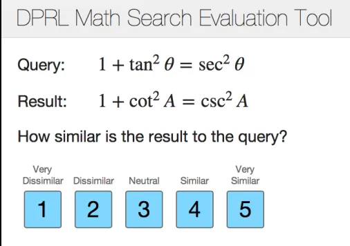
system for 10 queries. The participants were shown one query and result

answer on a 5-point Likert scale (See Figure 4.1). We asked the participants

to score by similarity rather than relevance because relevance is dependent on

the search task, which is beyond the scope of this experiment.

Figure 4.1: Screenshot of the evaluation tool used in the experiment.

The corpus used for the experiment was the Wikipedia corpus. The

queries were chosen by randomly sampling a larger set of queries from the

corpus, and picking from this 10 that represented diversity in size, type of

structure, and field (see Table 4.1). Due to time constraints in the

experi-ment, we were unable to compare all of the ranking functions we developed.

We conducted an informal experiment beforehand and determined that the

best-performing ranking functions were F-Measure, Distance, and Prefix. The

experiment was thus a comparison between Tangent with these three ranking

functions and Yuan and Zanibbi’s Lucene-based system (henceforth referred

# Query 1 ρ_e

2 u¯= (x, y, z) 3 1 + tan2_{θ = sec}2_θ

4 cos(θE) = e−T R/T1

5 a =gm1−m2

m1+m2

6 R_abf(x)dx=F(b)−F(a).

7 1/6, p1/28, −p12/7, 0, 0, 0, 0, 0

8 Pn

i=mai =am+am+1+am+2+· · ·+an−1+an.

9 f(x;µ, c) =p _c

2π e−

c

2(x−µ) (x−µ)3/2

10 D4σ = 4σ = 4

r_R∞

−∞

R∞

−∞I(x,y)(x−¯x)2dx dy

R∞

−∞

R∞

−∞I(x,y)dx dy

Table 4.1: List of queries used in the experiment.

The experiment was run in person, one participant at a time, through a

web-based evaluation tool (see Figure 4.1). Before the experiment, participants

were asked to fill out a short demographics survey. Then, they completed a

short familiarization exercise, wherein they scored 5 results from each of 2

queries. These responses were excluded from analysis. After this task was

complete and any questions were answered, they began the main experiment.

In addition to the scores, we also recorded the time it took the participant for

each query. Finally, they were asked to rate the difficulty of the task and to

describe their process of scoring. The task took approximately 30 minutes and

participants were paid $10 for their time.

To save time, any results found by both systems were only scored once.

This allowed us to include results from three of our ranking functions without

different rankers. After deduplication, the participants were asked to score

214 results, 10 of which were for the familiarization exercise. To ensure a fair

comparison, both the order of the queries and the order of the results were

randomized for each participant.

4.1.2 System Performance

Indexing and retrieval speed is simpler to evaluate, as it can be directly

measured. Indexing time was tested using the full Wikipedia corpus

(approx-imately 482,000 expressions). Retrieval time was tested using the 10 queries

from the experiment and the same corpus. We analyzed system clock time as

opposed to operation counts because we are just interested in if the system is

fast enough, and for that we need actual clock times. Operation counts would

be more appropriate for a formal performance comparison. Using clock time

has the drawback of introducing noise into our timings and being dependent

on specific hardware. The former can be mitigated with multiple trials and

the latter is reasonable considering our goal.

As indexing speed is only important for the initialization of the system,

it is the less important of the two quantities being measured. It is still an

interesting and important quantity. It would be difficult to experiment with

the system if it takes days to index the corpus. Retrieval speed is much more

important to the success of the system. It is mostly binary: either the system

is fast enough to be used in real time (queries running in under approximately

4.2

Results

4.2.1 Demographics and Survey Responses

20 students and professors participated in the experiment. 15 (75%) of

the participants were male. 15 (75%) were between the age of 18 and 24, three

(15%) were 25-34, and one (5%) was 35-44. All participants were from fields

in science and technology, with 13 (65%) in computing, 5 (25%)in science, and

2 (10%) in mathematics. Students and faculty in these fields were targeted

because they represent a group that might find a math search engine useful in

their work. 1 participant (5%) found the task very difficult, 11 (55%) found

it difficult, 7 (35%) were neutral, and 1 (5%) found it easy. When asked to

describe how they evaluated the results, 17 (85%) mentioned using visual

sim-ilarity and 10 (50%) mentioned semantic meaning. The additional comments

mostly described how difficult the users found the task, which aligned with

their ratings.

4.2.2 Search Result Scores

Our result scores are from a Likert scale, which is ordinal data with

no inherent numeric value. Whether it is valid to use Likert data as numeric

values for statistical analysis remains an open question. We will avoid doing

this, as we can test our hypothesis with the more conservative approach of

treating it only as ordinal data. We can thus not directly apply an analysis of

variance (ANOVA) test to our results. In order to get around this, we binarize

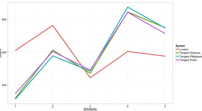
Figure 4.2: Score counts by system for 10 results each for 10 queries.

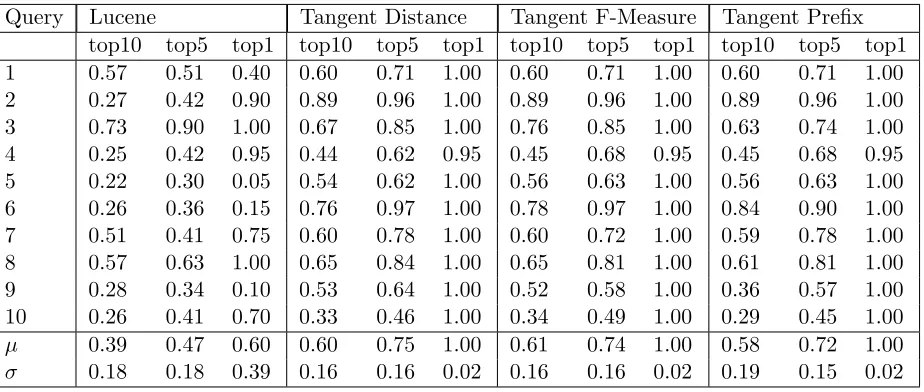
relevant (scored neutral or worse). With this, we can then calculate the

top-10, top-5, and top-1 precision for each query. Table 4.2 shows these values for

each system.

A two-way ANOVA test looking at the effects of the system and query

on average top-10 precision shows a very strong effect of the system (p <

2.2∗10−16_{) as well as of the query (p <8.9∗10}−16_{). There was no interaction}

effect found between the system and query (p < 0.205). Running pairwise

t-tests (using the Bonferroni correction for multiple comparisons), we see that

there is a significant difference is between Lucene and each of the three Tangent

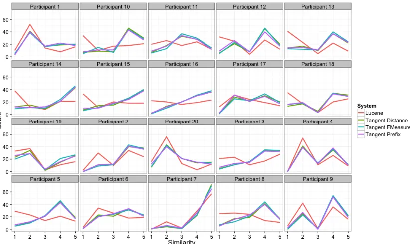
Figure 4.3: Score counts by participant and system.

Figure 4.4: Score counts by query and system.

The ANOVA test is unnecessarily conservative for two reasons: firstly

sec-Query Lucene Tangent Distance Tangent F-Measure Tangent Prefix top10 top5 top1 top10 top5 top1 top10 top5 top1 top10 top5 top1 1 0.57 0.51 0.40 0.60 0.71 1.00 0.60 0.71 1.00 0.60 0.71 1.00 2 0.27 0.42 0.90 0.89 0.96 1.00 0.89 0.96 1.00 0.89 0.96 1.00 3 0.73 0.90 1.00 0.67 0.85 1.00 0.76 0.85 1.00 0.63 0.74 1.00 4 0.25 0.42 0.95 0.44 0.62 0.95 0.45 0.68 0.95 0.45 0.68 0.95 5 0.22 0.30 0.05 0.54 0.62 1.00 0.56 0.63 1.00 0.56 0.63 1.00 6 0.26 0.36 0.15 0.76 0.97 1.00 0.78 0.97 1.00 0.84 0.90 1.00 7 0.51 0.41 0.75 0.60 0.78 1.00 0.60 0.72 1.00 0.59 0.78 1.00 8 0.57 0.63 1.00 0.65 0.84 1.00 0.65 0.81 1.00 0.61 0.81 1.00 9 0.28 0.34 0.10 0.53 0.64 1.00 0.52 0.58 1.00 0.36 0.57 1.00 10 0.26 0.41 0.70 0.33 0.46 1.00 0.34 0.49 1.00 0.29 0.45 1.00

µ 0.39 0.47 0.60 0.60 0.75 1.00 0.61 0.74 1.00 0.58 0.72 1.00

σ 0.18 0.18 0.39 0.16 0.16 0.02 0.16 0.16 0.02 0.19 0.15 0.02

Table 4.2: Top 10, Top 5, and Top 1 precision by query and system.

ondly because the binarization process loses information. Because the

differ-ence between Lucene and Tangent is so great, the test is perfectly valid and

able to detect the difference. A Friedman test addresses both of these

con-cerns. As a non-parametric test based on ranking the given scores, it is able

to operate on the ordinal Likert scores directly. Additionally, the test allows

blocks, where there is a source of variability between the blocks that is not

important in the experiment. The blocks are ranked individually and thus

the unwanted variability does not affect the result of the test. In our case,

the blocking factors will be the query and the participant, the two sources of

variability that we identified earlier. The p-value for the Friedman test is even

stronger than the ANOVA result - it is a smaller value than our statistical

4.2.3 Response Times

In addition to the scores directly given by the participants, we also

collected the time it took each participant to score each result. As some

results were shared between systems and only displayed to each user once, the

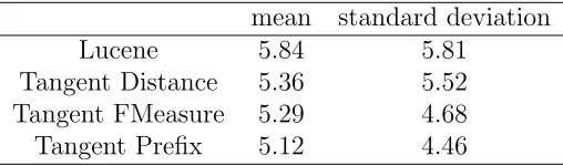
timings were likewise counted for each system with that result. An ANOVA

test on the timings by system showed that with high confidence (p <0.00007)

there is a significant difference between the systems. Specifically, from a t-test

(Bonferroni correction) post-hoc, there is a difference between Lucene and each

of the three Tangent systems, with p-values of 0.018, 0.0037, .000053 between

Lucene and Distance, F-Measure, and Prefix respectively.

mean standard deviation

Lucene 5.84 5.81

Tangent Distance 5.36 5.52

Tangent FMeasure 5.29 4.68

Tangent Prefix 5.12 4.46

Table 4.3: Response times by system (in seconds).

There is also a strong correlation between the scores given to and time

taken to score each result. As can be seen in Figure 4.5, participants took

longest to score the expressions that were not obviously similar or dissimilar.

This intuitively makes sense, as less thought is required if the expressions are

Figure 4.5: Response times by score.

4.3

Performance Metrics

As Lucene is a robust, mature, and heavily-optimized search engine,

the Lucene-based system is much more performant than Tangent. It is faster

for both indexing and searching, and the index is far smaller. But while

Tangent is clearly slower than Lucene, it is not unusably slow. Indexing the

Wikipedia dataset took 53 minutes - much slower than Lucene’s 7 minutes 44

seconds, but perfectly workable for a one-time task. The average query time

for the 10 queries used in the experiment is ∼_{1.5 s with a standard deviation}

of ∼_{1 s. This is well within our stated goal of being fast enough to be used}

in real time. Query time is dependent on the size of the query and number

of matches, but the even the largest (slowest) queries we tested took under 3

seconds. Tangent’s index for the Wikipedia dataset used 6.19 GB of memory

while Lucene’s on-disk index was a much smaller 107 MB (Tangent does not

4.4

Discussion

The results confirm both parts of our hypothesis. The ANOVA test (on

computed precision) and Friedman test (on raw scores) both reject the null

hypothesis and the associated post-hoc tests show that all three Tangent

varia-tions produce better precision-at-k values than the Lucene-based system. Our

performance comparison shows that while slower, performance in all categories

is sufficient for real-world use.

Both by looking at the graphs and the statistical tests, we can see that

our result is clear: Tangent’s results are better than Lucene’s (Appendix A

contains results for each query). While our scores are for the similarity between

the query and result, there is intuitively a very strong correlation between

similarity and relevance. If a resultlooks similar the query, we propose that it

is more likely tobe similar to the query.

The comparison between the various ranking functions was surprising

and less conclusive. We only tested three (F-Measure, Distance, and Prefix),

but IEF and Recall both performed worse than the others in a prior, informal

comparison. None of the three we did test were shown to be significantly

different. Considering this, we recommend the F-Measure ranker as it is the

simplest and (one of) the best performing.

Several trends are apparent in the scores obtained from the experiment.

By looking at the scores by participant (Figure 4.3) and by query (Figure 4.4),

par-ticipants scored expressions much higher on average than others, and several

avoided the “neutral” score. The scores vary between queries even more: in 5

of the queries (queries 2, 4, 5, 6, and 9), Tangent performs much better than

Lucene, but the scores in the other 5 queries are much closer. Additionally,

both systems perform poorly in query 10.

But while there was a lot of variation between participant and between

queries, Tangent’s scores were almost always higher. There are no individual

participants or queries for which you could argue that Lucene performs better.

Looking at the scores by query, we can put the queries in two categories: 5

where Tangent and Lucene score roughly as well as each other, and 5 where

Tangent does much better. What we can draw from this is that while Lucene

sometimes can find good matches, Tangent’s results are much more consistent.

This is important for a search engine, as a system that only returns good results

for half of the queries would be frustrating to use.

The performance analysis shows that while slower, Tangent is not

un-tenable for real-world use. The high memory usage necessitates a modern

computer that can address more than 4 GB of memory, but most current

computers are capable of running Tangent well. Both indexing and query

speed are good enough for the system to be used as an actual search engine.

Additionally, there is a few decades’ research in index compression and

opti-mization for text search that can largely applied to Tangent (see future work).

It is likely that a much more optimized system could be comparable to Lucene

compare our query speed with Kamali and Tompa’s results [4]. In an index

that is roughly twice the size as ours, their system is roughly twice as fast

as Tangent (∼_{800ms vs} ∼_{1500ms per query). In the same comparison, Sojka}

and L´ıˇska’s MIaS [14] is even faster, at∼300ms, and other various text-search

and exact match systems take between 200 and 400ms. This speed difference

could be a problem for larger indexes, but we can probably narrow the gap

significantly with some optimization.

4.5

Summary

The experiments described in this section confirmed both parts of our

hypothesis. The system provides high-quality search results and does so

rela-tively efficiently. There is, however, much room for improvement in both areas

Chapter 5

Future Work and Conclusion

5.1

Future Work

5.1.1 Performance Optimizations

While the performance of Tangent is acceptable, there are many

op-portunities for improvement. The most obvious is to reimplement the system

in a higher-performance language than Python. This is actually not as

im-portant as it might appear, because most of the query time is spent reading

data from Redis (which calls C libraries). Another possibility would be

stor-ing the index directly in memory, rather than indirectly through Redis. We

briefly experimented with both approaches (using the Go language), but very

surprisingly, query times were similar between the current Python-Redis and

the in-memory Go implementations. This was however not an exhaustive test,

and implementation-specific speedups could be possible.

More interestingly, however, are the decades of research in

optimiza-tions for (text) information retrieval. Index compression in particular could

be a great boon to performance because the majority of the query time is

spent transferring the inverted lists from the Redis server. Storing the

docu-ment references in a compressed form (either Elias’ gamma code or a bytewise

of these lists, as would storing the differences between document identifiers

rather than the identifiers themselves. Additionally, we could define a more

compact representation for the Symbol Pairs, but most of the time is spent

moving the document identifiers.

Another technique that could be applied from text information retrieval

is parallelization. For an index the size of Wikipedia, a load-balanced set of

servers running the entire index would allow the system to scale to more users,

albeit without improving query time. For larger indexes, performance (query

time) starts to become unacceptable. For these, more work would be needed

to allow servers to only contain parts of the full index and communicate with

each other to present a final result.

5.1.2 Retrieval Improvements

There are several ways worth exploring to improve the quality of the

search results. A major limitation of Tangent is that it does not allow for

substitution of symbols. For example, a2 _{should be a partial match for b}3_{, as}

they are both a variable raised to an integer power. While we showed that the

structure surrounding the symbols needing substitution is generally enough for

Tangent to return good matches (see Query 2 in Appendix A), substitution

would likely improve the result quality further. This could be accomplished

by creating a separate substitution index where one or both of the symbols

is replaced by a more general symbol (e.g. VARIABLE, OPERATOR,

expressions would share the general symbols than the specific ones. This could

make the performance of the system much worse without a clever approach to

avoid this repetition.

Using our definition ofdh, Symbol Pairs must match this distance

ex-actly. This is not as reasonable for large values of dh (there is not much

difference between a pair being 8 or 9 symbols apart. It could be possible to

find more general matches if we binned the values for dh. Another approach

would be to search for pairs not only with exactly dh but also dh+ 1, dh−1,

and so on.

Our definition for dv in the Symbol Pair is lossy. If, for example, an

ABOVE relationship is followed by a BELOW relationship, dv will be 0, the

same as if there were two ADJACENT relationships. This would occur with

the (x, z) pair in the expressionxyz_{. A possible solution to this problem would}

be to define dv as a list of the baseline changes - for this example, dv would

be [ABOVE, BELOW]. It is not clear if this would greatly affect the results,

or even if the effect would be positive.

There are two possible problems with the way we generate the Symbol

Pairs. The first is that we do not generate Symbol Pairs between pairs that

are on separate branches of the SLT. For example, there is no pair between

the 2 and yinx2_{+y. Fixing this would require major changes to the Symbol}

Pair representation, and as these pairs tend to represent weak semantic

rela-tionships, might not be helpful. The second issue is that the number of pairs

unintentional effect of preferring well-connected matches seems to be positive,

it is not apparent why this particular weighting is ideal. It would be possible

to counter this effect (possibly to introduce another) by weighting each

Sym-bol Pair inversely proportional to the number of other SymSym-bol Pairs that use

either of the symbols in it.

Currently, Tangent does not support tables or matrices because they

cannot be represented well using a Symbol Layout Tree. One simple solution

would be to simply index each table cell separately, as its own expression.

Another approach would be to modify the SLT and Symbol Pair definitions

to allow for this structure.

Finally, it might be interesting to use geometric distances for dh and

dv instead of distances within the layout tree. We could render the expression

to find these distances. Doing this would change the general type of matching

that is being done, moving towards a directly visual match from a (somewhat)

semantic one. It is unknown if this would produce better or worse results, but

it would introduce to major problems. The first is that the distances would be

dependent on the font and font size. The second is that these distances would

then be real-valued and thus not able to be inserted into a table. Without a

solution to these problems, indexing would likely be unfeasible.

5.1.3 Additional Comparisons

Our system performed well in the comparison with the Lucene-based

It would be interesting to compare our search results with those of some of

the other systems mentioned in Chapter 2; Kamali and Tompa’s SimSearch [4]

and Sojka and L´ıˇska’s MIaS [14] would be good candidates.

5.2

Conclusion

Hypothesis: Implementing a math expression search

sys-tem using an inverted index on symbol pairs from layout

trees will: 1) yield more relevant results than text-based

retrieval, and 2) be fast enough for real time use.

We have shown evidence to strongly support both claims in the

hy-pothesis. Our novel approach to math expression retrieval yields high quality

search results and does so efficiently. Not only have we created a search system

that performs competitively today, we have introduced several new

opportuni-ties for future work (discussed below). Additionally, we introduced a rigorous

method for evaluating results in math expression retrieval using human

Query 1: ˜

ρ

Rank Lucene Tangent F-Measure Tangent Distance Tangent Prefix

1 ρ→eρ_e ρ˜ ρ˜ ρ˜

2 ρ˜ ρρ˜ ρρ˜ ρρ˜

3 (ρ,eVe) ρ→ρee ρ→eρe ρ→eρe

4 ρφψf ρ_e=ρ∗ ρ_e=ρ∗ ρ_e=ρ∗

5 Xe ρ˜(k) ρ˜(k) ρ˜(k)

6 Be ρ˜(r) ρ˜(r) ρ˜(r)

7 Mf ρ˜_uc(k) ρ˜_uc(k) ρ˜_uc(k)

8 te (ρ,_eVe) (ρ,_eVe) (ρ,_eVe)

9 (ρ, V)7→(ρ,_eVe) dρ˜(ρ) = 0 dρ˜(ρ) = 0 dρ˜(ρ) = 0

10 ρ_e=ρ∗ trRχ˜= ˜ρ ρ˜(1)·v=v trRχ˜= ˜ρ

Query 2: ¯

u

= (

x, y, z

)

Rank Lucene Tangent F-Measure Tangent Distance Tangent Prefix 1 f(¯u) =f(x, y, z) u¯= (x, y, z) u¯= (x, y, z) u¯= (x, y, z) 2 = R(z, dt)|x, y, zi u= (x, y, z) u= (x, y, z) u= (x, y, z) 3 (x∨y)(¯x∨z)(y∨z) = (x∨y)(¯x∨z) v= (x, y, z) v= (x, y, z) v= (x, y, z) 4 u¯= (x, y, z) r= (x, y, z) r= (x, y, z) r= (x, y, z) 5 z(x) = _dxdy(x) x= (x, y, z) x= (x, y, z) x= (x, y, z) 6 f(t,u¯) =f(t, x, y, z) F = (x, y, z) F = (x, y, z) F = (x, y, z) 7 P(X=x|Y =y, Z =z) = P(X =x|Z =z) r0 = (x, y, z) r0 = (x, y, z) r0= (x, y, z)

8 =H(p, q)·G(p, q)|_p=x λz,q=

y

λz ~x= (x, y, z) ~x= (x, y, z) ~x= (x, y, z)

9 P ={(x, y, z)|3x+y−2z= 10} x= (x, y, z)T (x, y, z) x= (x, y, z)T 10 z(x) =Q(y(x),_dxdy(x)) (x, y, z) x= (x, y, z)T _{(x, y, z)}

Query 3: 1 + tan

2

θ

= sec

2

θ

Rank Lucene Tangent F-Measure Tangent Distance Tangent Prefix 1 1 + tan2_{θ= sec}2_{θ 1 + tan}2_{θ= sec}2_{θ 1 + tan}2_{θ= sec}2_{θ 1 + tan}2_{θ= sec}2_θ

2 tan2θ+ 1 = sec2θ 1 + tan2y= sec2y 1 + tan2y= sec2y 1 + tan2y= sec2y

3 sec2θ= 1 + tan2θ _dθd tanθ= sec2θ _dθd tanθ= sec2θ _dθd tanθ= sec2θ

4 1 + tan2θ= sec2θ and 1 + cot2θ= csc2θ. 1 + cot2θ= csc2θ sec2θ= 1 + tan2θ 1 + cot2θ= csc2θ

5 cos2θ+ sin2θ= 1 , sec2θ= 1 + tan2θ 1 + cot2θ= csc2θ p1 + tan2θo

6 sin2θ+ cos2θ= 1 p1 + tan2_θ

o tan2θ+ 1 = sec2θ ±

√

1 + tan2_θ

7 cos2θ+ sin2θ= 1 ±√1 + tan2θ p1 + tan2θo 1 + cot2A= csc2A

8 1 + cot2θ= csc2θ 1 + cot2A= csc2A ±√1 + tan2_{θ 1 + cot}2_{y= csc}2_y

9 cot2θ+ 1 = csc2θ 1 + cot2y= csc2y dtanθ= sec2θ dθ = dx₃ . ±_√ 1 1+tan2_θ

10 x=rcosθ= 2asin2θ= 2atan2θ = 2at2 tan2θ+ 1 = sec2θ ±_√tanθ _{dtanθ= sec}2_{θ dθ=} dx_.

Query 4:

cos

(

θ

E

) =

e

−

T R/T

1

Rank Lucene

1 cos(θE) =e−T R/T1

2 cos(θE) =e−(d1+at)/T1

3 AFHAST =AFH∗AFT =e(Constant∗(RH n

s−RHon)∗_e(Ea/k)∗(1/To−1/Ts)

4 AFT =e(Ea/k)∗(1/To−1/Ts)

5 P(Ei) =g(Ei)/(e(E−µ)/kT + 1)

6 sinθc= [−K2±(K22−3K1K3)1/2]/3K3 1/2

7 G_T

2 =GT1 + (Cp −ST1)(T2−T1)−T2ln (T2/T1)Cp

8 1 = cos(3π/8)Axc T ,L+B

xc

T,L+ cos(π/4)E xc T ,L

9 IC =ISO(eVBE/VT−1)≈ISOeVBE/VT

10 Eθ[(θi−Xi)h(X)|Xj =xj(j6=i)] =

R

(θi−xi)h(x) ₂1_π

n/2

e−(1/2)(x−θ)T(x−θ)m(dxi)

Rank Tangent F-Measure Tangent Distance Tangent Prefix 1 cos(θE) =e−T R/T1 cos(θE) =e−T R/T1 cos(θE) =e−T R/T1

2 cos(θ) = 1 cos(θE) =e−(d1+at)/T1 cos(θ) = 1

3 cos(θE) =e−(d1+at)/T1 cos(θ) = 1 cos(θE) =e−(d1+at)/T1

4 cos(α) = 1 r·cos(θ) cos(α) = 1 5 r·cos(θ) µ=|cos(θ)| r·cos(θ) 6 x1=a1cos(θ) g=< cos(θ)> x1=a1cos(θ)

7 x2=a2cos(θ) x1 =a1cos(θ) x2=a2cos(θ)

8 P3

r=1cos( 2rπ

7 ) =

−1

2 x2 =a2cos(θ)

P3

r=1cos( 2rπ

7 ) =

−1 2

9 cos(α) = 1_k cos(α) = 1 cos(α) = 1_k 10 TL= _cosTN_(θ) TL= _cosTN_(θ) TL= _cosTN_(θ)

Query 5:

a

=

g

m

m

1

−

m

2

1

+

m

2

Rank Lucene Tangent F-Measure Tangent Distance Tangent Prefix