Multi-mission radar waveform design via a distributed SPEA2 genetic algorithm

(1)

Rochester Institute of Technology

RIT Scholar Works

Theses Thesis/Dissertation Collections

1-31-2012

Multi-mission radar waveform design via a

distributed SPEA2 genetic algorithm

Brent Josefiak

Follow this and additional works at:http://scholarworks.rit.edu/theses

This Thesis is brought to you for free and open access by the Thesis/Dissertation Collections at RIT Scholar Works. It has been accepted for inclusion in Theses by an authorized administrator of RIT Scholar Works. For more information, please [email protected].

Recommended Citation

(2)

I

Multi-Mission Radar Waveform Design via a Distributed SPEA2 Genetic

Algorithm

by

Brent Josefiak

A Graduate Thesis Submitted

in

Partial Fulfillment

of the

Requirements for the Degree of

MASTER OF SCIENCE

in

Electrical Engineering

Approved by:

(Dr. Vincent Amuso, Graduate Advisor)

(Dr. Sohail Dianat, Committee Member)

(Dr. Ferat Sahin, Committee Member)

(Dr. Sohail Dianat, Department Head)

January 31, 2012

DEPARTMENT OF ELECTRICAL AND MICROELECTRONIC ENGINEERING

(3)

II

-mRank : int MPIGenome +Evaluate() +CalculateObjectiveVectors() -MapGenesToVariables() -IlluminateRoI() -CalculateAverageRevistTime() -CalculatePulseIntegrationFitness() -CalculatePulseTiming() -CalculatePeakPosition() -NormalizeComplex() -CalculatePeakPower() -mPulseTiming -mNumCpi -mVideoPhaseHistory RadarGenome +SetConfiguration() +SetFactory() #InitializePopulation() #ExecuteAlgorithm() #SaveGeneration() -GaConfiguration -GenomeFactory BaseGa #ExecuteAlgorithm() #CalculateObjectiveVectors() #SortMembersByRawFitness() #CalculateDominated() #CalculatePopulationStrength() #CalculatePopulationRawFitness() #CalculatePopulationFinalFitness() #CalculateEnvironmentalPerformance() #CalculateKFactor() #PopulateMatingPool() #PerformMating() #PerformMutation() #EvaluateEndCondition() -mArchive -mPopulation -mLoopCnt SPEA2_ST +SetNumSlaves() #ExecuteAlgorithm() #CalculateObjectiveVectors() -mNumSlaves SPEA2_MPI «datatype» VectorGenomePointers 1 * «uses» +AllocateGenomeCopy() GenomeFactory +AllocateGenomeCopy() RadarGenomeFactory «uses» +SortMembersByObjective() +CalculateDensity() +UniformCrossover() +SortDistances() +SetRank() «interface» GenomeHelpers «uses» +GetFitnessFromMap() +LoadScenario() +SaveScenario() +InitializeRadarFitnessMaps() «interface» Scenario «uses» +GetParameter() +IsParameterDynamic() +GenerateRandomParameter() +GetCRLimits() +GetDRLimits() «interface» RadarParameters «uses»

Figure 1 C++ Radar Waveform Design Suite Class Diagram

Figure 1is a UML diagram laying out the relationship between the Genetic Algorithm, its

population members (Genomes) and the helper functionality supporting them. At the lowest

level, there are the Genome and BaseGa classes[14]. The specific algorithm implementations,

(8)

3 upon. The Genome class contains the genetic information required for a given problem, but not

the ability to interpret the encoded information; that task is left to a derived class.

New population members are constructed through a GenomeFactory class, which isolates

the algorithm from the problem specific genome implementation.[14] This factory is provided to

the algorithm as part of the initialization. Radar data and functions are contained in the

RadarGenome class that is derived from the base Genome. The radar members contain the ability

to translate their generic genetic information into radar specific parameters (azimuth angle,

center frequency, etc).

The GenomeHelper interface provides a layer of abstraction that manipulates the inner

workings of multiple genomes. This prevents the genetic algorithm from needing to understand

the inner workings of its genomes when it desires operations involving two or more genomes. An

excellent example of this is uniform crossover, where the algorithm provides the helper with two

genomes and, based on the scenario's crossover probability (provided as part of the scenario

initialization), the helper function handles the swap of genetic information. The other helper

functions in this class fall into this category of acting upon two or more genomes.

SPEA2_ST is the single threaded SPEA2 implementation derived from the BaseGa,

which implements and validates the original waveform design suite algorithm in C++. The

SPEA2 implementation acts upon two genome sets, the new member population and archive

pools. It contains the functionality required to calculate the raw fitness, strength and final

ranking of the populations.

SPEA2_MPI is the MPI compatible implementation of SPEA2, which re-implements the

algorithm to distribute genetic information from the master algorithm to a set of slave genomes.

These slaves are distributed across multiple cores so that the computationally intensive 2D IFFTs

required to calculate PSL and ISL can be run in parallel. When the current set of slave genomes

have yielded their fitness data, 0.0 to 1.0 values representing the success of that particular

member, it is transmitted back to the master. The master process then continues to calculate the

(9)

4

This functionality was overridden by the MPI implementation. It is here that data

is distributed to Slave processes.

Archive size correct

Fill in VPH

End condition

met Exit

Mating pair remaining Populate mating

pool

Uniform Crossover

Binary Mutate

Add to population

Truncate Add Dominated

Populate Archive Calculate Enviromental Performance CalculateObjective

Vectors (Archive ) CalculateObjective

Vectors (Population )

Yes No

Yes Exact

Small Large

No

Figure 2 SPEA2 ExecuteAlgorithm

Figure 2 and 3 highlight the changes to the Execute Algorithm and Calculate Objective

Vectors functions that were overridden from the original single threaded implementation.

(10)

5 pools off to the genome slaves. The total number of slaves is configurable at run-time and can

utilize as many cores as are available on a given grid implementation.

Member Available

Slave Available

All Results Received

Transmit Gene

Data

Receive Fitness

Data Yes

No

No Yes

Yes Exit No

Distribute Begin

Receive Gene

Data

Transmit Fitness

Data

Initialize From Gene Data

Calculate Objective Vectors Evaluate MPI_Isend()

MPI_Send()

[image:10.612.76.541.117.357.2]

Master Process (1) Slave Process (N - 1)

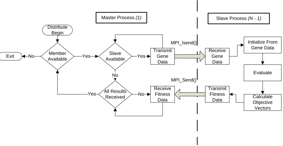
Figure 3 MPI Calculate Objective Vectors - Parallel Computation Distribution and Result Recovery

For a population of size Np and archive of size Na, an optimal number of processors

would be Np + Na + 1 = Copt. This allocates a core for every population member and one for

the master algorithm. The current software suite will not yield any benefit when there are more

cores available than combined population and archive members. See sections 6 and 7 for a

detailed analysis of the MPI performance improvement.

It should be noted that two different MPI transmission mechanisms are used when

transmitting gene data verses the returning slave generated fitness data. When the master is

distributing information to the various tasks it utilizes MPI_Isend, which is the non-blocking

send. As each slave process is known to be waiting at this point, the master can send the

information to each immediately without waiting for an acknowledgement back. This readiness

can be assured because synchronization occurs when the slave process calls MPI_Send (the

blocking call) to return the fitness data. As soon as the slave has returned its fitness data, it is

(11)

6

3. Scenario and Algorithm Configuration

A run of the test suite requires two files for configuration parameters, one that sets the

general genetic algorithm parameters and one to configure the scenario specific radar parameters.

These parameters are stored in human readable text files that are provided as arguments when the

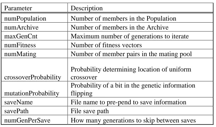
[image:11.612.119.496.244.466.2]

program is launched. General configuration information required by the BaseGa is listed in

Table 1, along with the description of each parameter.

Table 1 Base GA Configuration Format

Parameter Description

numPopulation Number of members in the Population

numArchive Number of members in the Archive

maxGenCnt Maximum number of generations to iterate

numFitness Number of fitness vectors

numMating Number of member pairs in the mating pool

crossoverProbability

Probability determining location of uniform crossover

mutationProbability

Probability of a bit in the genetic information flipping

saveName File name to pre-pend to save information

savePath File save path

numGenPerSave How many generations to skip between saves

Radar scenario parameterization is defined in a second file and loaded into a dynamic parameter

map during runtime initialization. This map allows each RadarGenome access to the scenario

configuration by indexing based on the requested parameter. If a parameter is dynamic for a

given scenario, it will contain all the potential values index-able by the genetic information of a

population member.

The first parameter in the scenario file is the random number seed. Saving the seed allows

a scenario to be reproduced again in the future. Given the same random seed value, arun of the

algorithm will produce identical results, asall of the randomness in the algorithm is based on the

pseudorandom “randn” functionality. Changing this value is necessary to examine how different

populations would respond to the same scenario.

(12)

7 determines the length in seconds the scenario will model. Taken with Pulse Repetition

Frequency (PRF) and pulses per interval, this value determines the number of Coherent Pulse

Intervals (CPI) a waveform will transmit.

The next line in the configuration file currently contains 4 bits, which toggle the various

fitness metrics on and off. In order, these bits enable (1) or disable (0) the use of the Peak Side

Lobe (PSL), Integrated Side Lobe (ISL), Average Revisit Time and Integrated Pulses fitness

functions. Any combination of these can be can be used, but the total number of enabled fitness

functions must match the number provided to the base genetic algorithm. Failure to match these

parameters will cause the GA to use the first n fitness vectors, where n is the number specified

within the GA’s configuration file.

The lines after this are the 22 configuration parameters that describe a radar scenario.

Each line is a comma delimited string and contains a digit stating which parameter it is (0 -21),

next a digit stating whether it’s an integer (0) or double (1) parameter, then the number of values

that parameter can assume, and finally the values themselves. Each parameter can assume

between 1 and 232 possible values in steps of powers of 2. If only one value is provided, the

parameter is considered static and not included in the genetic information of population

members.

Parameters for the CPI (enumeration 0), Number of Apertures (enumeration 1), PRF

(enumeration 6) and the total simulation time are used to determine the length of the genetic

information of a given member. When any of these parameters are dynamic, and thus contained

in the genetic information, the number of alleles used by population members will vary. When a

population member is initially generated, all the dynamic parameters of a given CPI are

randomized and it is pushed onto a vector. After each CPI is generated, the time elapsed is

checked, the number of pulses divided by the selected PRF, to ensure it does not exceed the total

simulation time. If the number of apertures is dynamic, the other dynamic parameters are

repeated A times for a given CPI, where A is the number of active independently steerable

apertures. Despite the repetition of all dynamic parameters, each CPI in a multiple aperture

scenario can only select one PRF and number of CPIs (if these parameters are dynamic). This

limits the multiple apertures to mainly altering the steering parameters.

The remainder of the parameters laid out in the scenario configuration file focus on

(13)

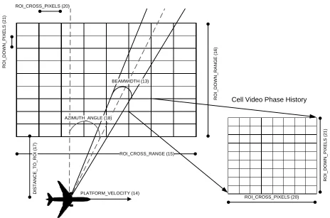
8 platform is the plane carrying the radar waveform, and its movement is defined as a line along

the ROI cross range at a speed specified by parameter 14 in meters per second. The

perpendicular distance from the ROI is defined in meters by parameter 17.

ROI_CROSS_RANGE (15) R O I_ D O W N _ R A N G E ( 1 6 )

Region of Interest

D IS T A N C E _ T O _ R O I (1 7 ) ROI_CROSS_PIXELS (20) R O I_ D O W N _ P IX E L S ( 2 1 ) PLATFORM_VELOCITY (14) ROI_CROSS_PIXELS (20) R O I_ D O W N _ P IX E L S ( 2 1 )

Cell Video Phase History

AZIMUTH_ANGLE (18)

[image:13.612.74.538.163.470.2]

BEAMWIDTH (13)

Figure 4 Scenario Parameter Representation

The other scenario parameters highlighted in Figure 4 are the ROI region parameters,

which define the total cross and down range (15/16) in meters, as well as the size of a pixel

within that region (20/21). Each one of these cells is made up of a VPH array of size defined by

parameters 20 and 21, typically 128 x 128. The final parameter required for the computation of

PSL and ISL are the IFFT cross and down-range dimensions, which define the resolution and

complexity of the 2D - IFFT calculation.

4. Fitness Mapping

Other than the two configuration files defining algorithm and scenario parameters, there

(14)

9 mapping between a scenario specific parameter and the 0.0-1.0 fitness metric used by the SPEA2

algorithm. Currently there are two formats for these files, which is stated in the first line of the

file; 0 for an integer based mapping and 1 for a floating point implementation. After the type is

determined, the next line tells how many data points the file contains and the maximum value

possible for the objective value. Each of the subsequent lines then listsan objective value (in

either integer or double format) and its corresponding fitness value. When the radar member

maps an objective to fitness value, if it does not match one of the points provided in the map, it

takes the linear interpolation between the two closest objective values to determine the correct

fitness value.

4.1.Genetic Representation

Each base genome contains all the genetic information required for a given scenario and,

once the member has been evaluated, its performance data. Base genetic information is stored in

an array of 32-bit values. Each 32-bit allele will be used by the problem specific

(RadarGenome) class to map to a scenario relevant value. These alleles are capable of mapping

up to 232 different parameters, should the functionality be desired, but most parameters are kept

to around 5-bits or 32 values. The one restriction on parameter mapping in the current

implementation is that the scenario must use 2N mappings exactly (where N is 0-32); non power

of 2 mappings results in an invalid configuration. This constraint was placed to prevent

mutation from generating an allele without a valid parameter mapping.

4.2.Uniform Crossover Operator

Uniform crossover is applied to each mating pair selected for the new population pool.

The crossover point is selected based on the smaller parent genome and the crossover

probability, which is typically 0.5, so that any location is equally likely to be the crossover

location[2]. A check for the smaller parent is required for situations when pulse per CPI or PRF

are dynamic and can alter the total number of genes present in a given population member.

Valid crossover points must be on allele boundaries, but are not constrained by where a CPI or

(15)

10 4.3.Binary Mutation Operator

The binary mutation operator works based on a probability of flipping provided by the

configuration file and the number of bits per allele defined in the scenario configuration. After

the members of the mating pool have undergone uniform crossover, each is subjected to

mutation. This mutation operator iterates over each bit in the population member's genetic

information; then a random number is generated and checked against the range defined by the

GA's mutation probability. If the value is in the specified percentage of the random range, then

the bit is flipped by XORing the current allele with a 1 shifted to location of the current target

bit.

4.4.Radar Genome Mapping

The Radar Genome takes each allele to be an index into the scenario’s dynamic

parameter map. The total number of alleles in a given member must be a multiple of the number

of dynamic parameters in a given radar scenario.

The radar member class uses the static scenario parameters as well as the dynamic values

mapped to its genetic information to construct a coherent pulse interval timing sequence. This

sequence defines at what position the target platform initiates a given CPI, where it is aimed, and

how many pulses are triggered at a given PRF, which defines at what platform location and times

a waveform burst will be triggered.

5. Radar Scenario Calculation.

Once this burst information is constructed, the platform location and antenna steering

parameters are used to determine which cells of the region of interest (ROI) are illuminated in a

given coherent pulse interval (CPI). This information is stored in a 2 dimensional Pixel

Illumination Vector where each ROI cell has a vector that is pushed back with new pulse timing

each time it is illuminated. After it is known which bursts illuminate a given ROI cell, the Video

Phase History (VPH) can be filled in, and the MTI revisit time parameter can be calculated [1].

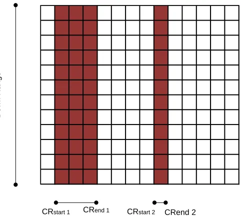
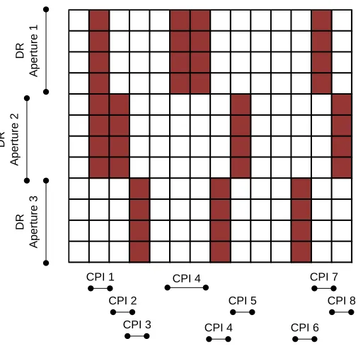
To illuminate the VPH, two factors come into play. The cross range VPH cells are

(16)

11 on the bandwidth and number of apertures. As highlighted in Figure 4, the VPH dimensions are

defined by the down and cross pixel count. When a single aperture is used, the down range, or

column as seen in Figure 5, is fully illuminated. Multiple apertures cause the down range

dimension (rows) to be divided up so that the bandwidth is allocated evenly amongst

sub-apertures as seen in Figure 6. The cross range illumination is determined by the following

equations:

Where is the total simulation time and is the time a given CPI begins to illuminate the

ROI. The and variables are used to index into the VPH and determine which

cross range (columns) are illuminated by the current CPI, as can be seen in Figure (x, y).

D

o

w

n

R

a

n

g

e

[image:16.612.191.432.434.651.2]

CRstart 1 CRend 1 CRstart 2 CRend 2

(17)

12

D

R

A

p

e

rt

u

re

1

CPI 1 CPI 4

D

R

A

p

e

rt

u

re

2

D

R

A

p

e

rt

u

re

3

CPI 2

CPI 3 _{CPI 4} CPI 5

[image:17.612.177.430.121.366.2]

CPI 6 CPI 8 CPI 7

Figure 6. Multiple Sub-Aperture Illumination.

One may notice that we are iterating across all the CPI's twice in the algorithm shown in

Figure 7, unfortunately memory limitations on the size of the VPH limited the number that could

be allocated. The smaller scenario, where a 256x256 2D-IFFT is computed, necessitated

256(DR) * 256(CR) * 8(Bytes per double) * 2 (complex) = 1 MB of contiguous memory per

VPH buffer, two of which are required per ROI cell (one for input and one for output).

Although several could be allocated, not enough were available to provide one for every ROI

cell, so we are forced to iterate over the CPI two times.

Once all the CPIs that illuminate a given ROI cell have illuminated it, the 2-dimensional

IFFT can be run across the VPH. The 2-dimensional Inverse FFT is calculated using the FFTW

library developed by Matteo Frigo and Steven Johnson of MIT. This library is upheld by

benchmarks as the fastest available FFT implementation and is licensed for use in Matlab. The

IFFT dimension is typically twice that of the VPH pixel count so that there is sufficient

resolution to calculate PSL and ISL. Were further computing power available, increasing this

(18)

13 The complex information generated by this operation is normalized to a power mapping,

which is then used to find the PSL and ISL performance. In order to calculate PSL and ISL, the

main power lobe is located and the total power contained within it is summed. The remainder of

the power mapping is then summed in order to calculate the ISL. While iterating across the

remaining pixels, the maximum value found is saved and used to calculate the PSL.

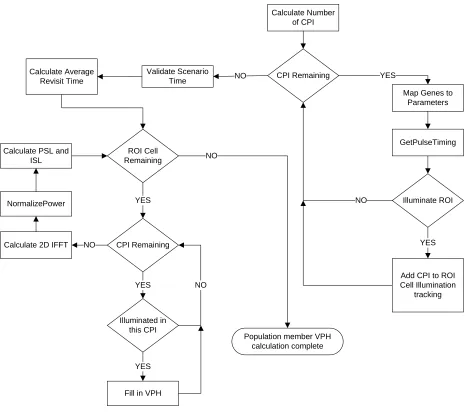
Map Genes to Parameters CPI Remaining

Calculate Number of CPI

YES

GetPulseTiming

Illuminate ROI

Add CPI to ROI Cell Illumination

tracking YES NO

Calculate Average

Revisit Time NO

ROI Cell Remaining

CPI Remaining YES

Calculate 2D IFFT NormalizePower

NO Calculate PSL and

ISL

Illuminated in this CPI

YES

Fill in VPH YES

NO NO

Population member VPH calculation complete Validate Scenario

[image:18.612.73.539.214.629.2]

Time

Figure 7. Radar Genome Evaluation

Once the radar calculations have been completed the performance data is gathered.

These values are then used to index a fitness map, which normalizes performance into a fitness

(19)

14 performance of population members. In the case of the MPI implementation it is this normalized

fitness value that is returned to the master. Further detail on how SPEA2 uses this fitness

information to select the fittest members for addition to the archive can be found in [3].

6. MPI Performance Validation

Just as the initial C++ implementation was validated against the original Matlab

implementation, so too was the grid implementation validated against previous results. The

resulting genetic algorithm performance, once differences in CPU performance were normalized,

were in line with the expected parallelization gains. The MPI grid used for the simulations

presented later in this paper had only had 30 cores available, while most test runs contained a

population size of 100 and archive size of 20. This is well below the Copt found previously, so it

becomes important to understand the distribution scheme and its affect on parallelization.

When testing began on the grid one immediate revelation was that running a single

threaded implementation was slower than an identical run to generate the single threaded results

of previous C++ simulations. This was caused by a CPU difference and the difference was

baselined by running a series of 256 by 256 2D-IFFT. A single grid core was capable of

executing this in 10ms, which is 3x slower than the previous implementation. Despite this

silicon setback the "embarrassingly parallel" nature of the genetic algorithm scenario allowed the

other 27 cores to prove the value in a distributed algorithm.

As noted previously, information is distributed to the slaves in batches based on how

many slaves have been constructed. This batch scheduling approach means that a speed-up only

occurs as slaves increase by least common multiples of the total population size.

Thus the total speed up versus the single threaded implementation is given by:

7. MPI Grid FFT Performance

In order to understand the time required to compute the 2D-IFFTs of a generation, a

(20)

15 to compute its IFFT averaged over a hundred runs. The results from these runs can be seen in

the following Table 2.

Table 2. IFFT Time

VPH CR

IFFT2 CR

Time Per Transform (sec)

Time Per Member - 45m x 1000m (sec)

Time Per Member - 45m x 1000m (min)

128 256 0.0198682 66.161106 1.1026851

256 512 0.04555384 151.6942872 2.52823812

512 1024 0.11810853 393.3014049 6.555023415

1024 2048 0.26291108 875.4938964 14.59156494

2048 4096 0.56116136 1868.667329 31.14445548

These test runs were all computed with a VPH down range dimension of 128 and IFFT

down range 256. The cross range dimension was repeatedly doubled from an initial IFFT of 256

up to 4096. One can see that the 128 x 256 transform required 0.0198 seconds to complete,

while the 2048 x 4096 required 0.5611 seconds per calculation.

The large 45m by 1000m ROI scenario requires each member to calculate 3330

2D-IFFTs, yielding the time required per member found in columns 4 and 5. Using the equation

generated in the previous section, one can determine that running a population size of 120 (20

archive plus 100 mating population), at the 256 by 512 size would require 51 minutes per

generation in pure FFT calculations.

When running the later SAR scenarios, this theoretical number was proven to be correct

with each generation requiring 55-56 minutes to complete. A full real-life SAR mission would

require the 45m by 1000m scenario to run with a VPH cross range of at least 2048 to provide a

column to each CPI pulse. Calculating this scenario with the current grid would require 622.88

minutes per member, or over 10 hours per generation.

8. SAR C++ Validation

The C++ SPEA2 waveform suite was first validated against the original SAR mission. In

this scenario, a platform illuminates a 45m by 30m region of interest in a 0.346 second run. The

original fitness mappings for PSL and ISL to the 0.0 to 1.0 fitness value were reused by the C++

implementation. Table 2 lists all the relevant parameters including the dynamic azimuth angle,

which is encoded in the genetic material of each population member. Running this scenario has

(21)

16 Figure 8 is the Illuminated VPH for the center cell of an archive member of the randomly

generated initial population. Note its relatively sparse illumination – only a small number of the

waveform’s CPIs were landing within the ROI. Contrast this with Figure 9 and one can see how

the 350 generations have found genetic material, which better illuminates the ROI cell. This

yields a significant improvement in PSL and ISL.

The improvement in fitness performance is illustrated in Figure 10. Over the course of

350 generations, the PSL and ISL have both improved by 6-7dB, which results in a fitness

improvement of 0.3-0.4. The fitness improvement of SPEA2 in this mission is not linear as most

of the growth occurs within the first 50 generations, while the remaining 300 offer a fraction of

growth. Understanding when fitness improvement tapers off allows for testing scenarios to an

optimal generation count and once this has been reached a new scenario can be tested more

[image:21.612.186.430.353.701.2]

quickly.

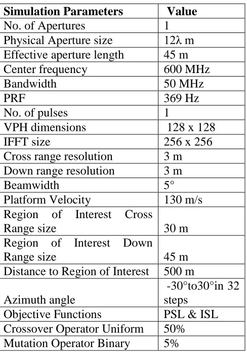
Table 3. SAR Parameters

Simulation Parameters Value

No. of Apertures 1

Physical Aperture size 12λ m

Effective aperture length 45 m

Center frequency 600 MHz

Bandwidth 50 MHz

PRF 369 Hz

No. of pulses 1

VPH dimensions 128 x 128

IFFT size 256 x 256

Cross range resolution 3 m

Down range resolution 3 m

Beamwidth 5°

Platform Velocity 130 m/s

Region of Interest Cross

Range size 30 m

Region of Interest Down

Range size 45 m

Distance to Region of Interest 500 m

Azimuth angle

-30°to30°in 32 steps

Objective Functions PSL & ISL

Crossover Operator Uniform 50%

(22)

17 Figure 8. Initial VPH for the center cell of the ROI. Figure 9. Final VPH for the center cell of the ROI.

Figure 10. Initial and Final Archive Population Fitness

Figure 11. SAR Maximum Member Fitness Improvement

20 40 60 80 100 120

20 40 60 80 100 120 Cross Range

(Yellow = Illuminated, Black = Not Illuminated)

D ow n R a nge

20 40 60 80 100 120

20 40 60 80 100 120 Cross Range

(Yellow = Illuminated, Black = Not Illuminated)

D ow n R a nge

0 0.2 0.4 0.6 0.8 1

Integrated Side Lobe Fitness

P e a k S ide L obe F it ne ss Initial Population Final Archive

0 50 100 150 200 250 300 350

(23)

18 Figure 11 illustrates the rate of change for the ISL and PSL fitness, where ISL continues to

improve throughout the generations, while PSL plateaus after 50 generations and sees only

marginal (1.5%) improvement.

The performance generated in the simple SAR scenario reproduces the previous [2] work

and shows the viability of the new C++ model for improving PSL and ISL.

9. MTI C++ Validation

The purpose of reconstructing the MTI mission in [1] is to baseline the functionality of the

new implementation against known results. The scenario parameters in Table 3 are used to run a

MTI mission where revisit time and number of pulses are used as the fitness functions in a 3

second run-time scenario.

Table 4. MTI Scenario Parameters

No. of Apertures 1

Bandwidth 50 MHz

PRF 369 Hz

No. of pulses 1, 8, 16, 32

IFFT size 256 x 256

Beamwidth 5°

Range size 1000 m

Range size 45 m

Distance to Region of

Interest 500 m

Azimuth angle

-60° to 60° in 32 steps

Objective Functions

Revisit & Pulse

Timing

Crossover Operator

Uniform 50%

(24)

19 The C++ implementation was able to quickly complete the MTI mission and rapidly

improved the performance of the archive population members. Comparing against [1] does

highlight a discrepancy in the fitness values achieved by the final archive population. Initial

random populations for both the original Matlab and new implementation have an average fitness

of ~0.5 for both Pulse and Revisit time. After one hundred generations, the Pareto optimal front

achieved by the original implementation is at around 0.6 to 0.8. While the new waveform design

suite has measured its final archive members to have 0.98 Revisit fitness and 0.9 Pulse fitness.

This performance is shown in Figure 12.

This growth is also achieved rapidly; in Figure 6 one can see that the revisit fitness has

approached its maximum within 10 generations. When implementing the PSL and ISL

calculations for the SAR mission, the original Matlab implementation was directly ported to C++.

Pulse fitness however was calculated with a new algorithm and this may explain some of the

fitness discrepancy. Originally the pulse fitness was found by calculating the average number of

pulses in each ROI cell, then averaging over the total number of ROI cells. The C++ algorithm

assigns a fitness value (between 0.0 and 1.0) to each pulses count per CPI type, and then

determines how many of each pulse count type occur in a given member. Averaged over the total

number of CPI, the summation of the fitness value by the pulse count is used to determine each

member’s Pulse fitness.

The results of the MTI mission are evolved successfully by the new suite and achieve an even

(25)

20 Figure 12. MTI Initial versus Final Archive Fitness (100 Generations)

Figure . MTI Maximum Member Fitness Improvement.

10.SAR MPI C++ Validation

Once the MPI extension was completed, the initial small scale SAR scenario was

re-executed to validate the distributed algorithm. The parameters were kept identical to the initial

SAR scenario, but re-run on the grid system to ensure that similar fitness improvement was

observed. The resulting fitness improvement and rate of fitness improvement can be observed in

the following figures.

0 0.2 0.4 0.6 0.8 1

P

ul

se

F

it

ne

ss

Revisit Time Fitness Initial Population

Evolved Archive Population

0 20 40 60 80 100

0 0.2 0.4 0.6 0.8 1

F

it

ne

ss

P

e

rf

or

m

a

nc

e

Generation

(26)

[image:26.612.316.465.530.685.2]

21 Figure 13. SAR Fitness Improvement per Generation

Figure 14. SAR Maximum Member Fitness Improvement

Figure 15. Initial VPH for the center cell of the ROI. Figure 16. Final VPH for the center cell of the ROI.

0 50 100 150 200 250 300 350 400 450 500 0 0.2 0.4 0.6 0.8 1 F it n e s s P e rf o rm a n c e Generation PSL Fitness ISL Fitness

0 0.1 0.2 0.3 0.4 0.5 0.6 0.7 0.8 0.9 1 0 0.1 0.2 0.3 0.4 0.5 0.6 0.7 0.8 0.9 1 In te g ra te d S id e L o b e

Peak Side Lobe Initial Population

20 40 60 80 100 120

20 40 60 80 100 120 D o w n R a n g e

Cross Range (Yellow = Illuminated, Black = Not Illuminated)

20 40 60 80 100 120

[image:26.612.129.286.532.686.2]

(27)

22 Figure 17. Initial 2D IFFT Normalized Magnitude Figure 18. Final 2D IFFT Normalized Magnitude

Performance of the MPI implementation was nearly identical to the gains observed in the

single threaded implementation. Figure 8 is the Illuminated VPH for the center cell of an archive

member of the randomly generated initial population, while Figure 9 shows the VPH of an

archive member from generation 500. There has been a significant improvement (but comparable

to the single threaded implementation) in the illumination of the center cell. This yields a

significant improvement in PSL and ISL, as can be observed in Figures 10 and 11. The plots

show the 2D IFFT magnitudes of generation 0 and generation 500 and one can observe a

significantly higher resolution point source in Figure 11.

The improvements in PSL and ISL evident in Figures 17 and 18 correspond to the fitness

improvement observed in Figure 7. The PSL and ISL have both improved by 6-7dB, which

results in a fitness improvement of .4 for the ISL and .5-.6 for the RSL. This is a comparable

level of growth to the initial single threaded implementation, with a small amount of additional

improvement achieved in the additional 150 generations the MPI variant was able to run. The

growth rate remains front loaded with the greatest improvement in the first 75 generations, but

PSL continued to make modest gains for the remainder of the simulation.

11.MTI MPI C++ Validation

This scenario recreates the large MTI scenario, but distributing it with MPI. A 1000m by

45m region of interest was examined over a 3 second simulation evaluating with the revisit time

(28)

23 be run for 500 generations instead of the 100 used in the Matlab and initial C++

implementations.

Figure 19. MPI MTI Inivital versus Final Archive Fitness

Figure 20. MPI MTI Maximum Member Fitness Improvement

Examining the two figures above one can see a similar level of performance

improvement from the initial implementation, when comparing the first 100 generations. The

advantage of running for 500 generations appears to be twofold. First, the Pareto Optimal front

created by the final archive population covers a wider range of potential solutions, with most of

this spread across the Revisit time fitness, but also increased distribution in the Pulse fitness as

well. Second, the final improvement of the Pulse fitness has reached the maximum over the

course of the run. This simulation validated the ability of the MPI solution to run the MTI

scenario accurately and reproduce the previous results.

0 0.1 0.2 0.3 0.4 0.5 0.6 0.7 0.8 0.9 1 0 0.1 0.2 0.3 0.4 0.5 0.6 0.7 0.8 0.9 1 P u ls e F it n e s s

Revisit Time Fitness

Pulse Fitness versus Revisit Time Fitness Performance MTI Mission

Initial Population Evolved Archive Population

0 50 100 150 200 250 300 350 400 450 500 0 0.2 0.4 0.6 0.8 1 F it n e s s P e rf o rm a n c e Generation

Maximum Fitness Performance Improvement versus Generation MTI Mission

(29)

24

12.SAR MPI Increased Resolution

In this scenario the same parameters are maintained from the original SAR scenario,

except the VPH dimensions and IFFT size are increased. With a VPH dimension of 128 x 256,

and scenario time remaining at 0.346 seconds, each CPI illuminates two cross range columns.

The IFFT size was increased to 256x512 to retain resolution.

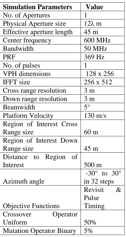
Table 5. SAR Increased Resolution Parameters

No. of Apertures 1

Bandwidth 50 MHz

PRF 369 Hz

No. of pulses 2

IFFT size 256 x512

Beamwidth 5°

Range size 30 m

Range size 45 m

Interest 500 m

Azimuth angle

-30° to 30° in 32 steps

Objective Functions

Revisit & Pulse

Timing

Crossover Operator

Uniform 50%

Mutation Operator Binary 5%

The results of this run can be observed in the following Figures where the final

improvement of generation 500 is comparable to that of the initial SAR run. PSL fitness has

improved from an initial average of 0.47 to 0.90, while ISL has gone from 0.61 to 0.81. The

largest discrepancy between the two runs comes from the initial fitness values, while the final are

(30)

25 conclusion that upping the size of the VPH while maintaining the same scenario time yields little

benefit to final performance.

Figure 21. SAR Fitness Improvement per Generation

13.SAR MPI Increased ROI Size 45m by 60m

This scenario keeps the increased VPH resolution of the previous solution, but pairs it

with an increased scenario ROI and flight time. Increasing the length of the scenario time to

0.692 seconds with the 369 Hz PRF caused each CPI to illuminate one complete cross range

column. Doubling the scenario time also allows the target platform to traverse twice the ROI

distance during the scenario, increasing the complexity of each population member's genome to

twice the number of chromosomes.

(31)

[image:31.612.200.415.92.497.2]

26 Table 6. SAR 45m by 60m Parameters

No. of Apertures 1

Bandwidth 50 MHz

PRF 369 Hz

No. of pulses 1

IFFT size 256 x 512

Beamwidth 5°

Range size 60 m

Range size 45 m

Interest 500 m

Azimuth angle

-30° to 30° in 32 steps

Objective Functions

Revisit & Pulse

Timing

Crossover Operator

Uniform 50%

Results from this scenario show that configuring the scenario time and PRF such that one

CPI illuminates a single cross range column (Figure 25, 26) will produce consistent performance

independent of the increase in ROI. Although this required doubling the amount of genetic

information, the run-time of this scenario was close to the higher resolution SAR 45m x 30m run.

This is due to the fact that most of the processing time is spent in the 2D – IFFT and not

determining which VPH bins are illuminated by a particular CPI.

Figures 23 and 24 show the rate of fitness improvement for PSL and ISL and the initial

versus final Archive member performance after 500 generations. PSL continues to be the fitness

metric most improved by the genetic algorithm, as it starts with a lower fitness and ends higher

(32)

27 final archive fitness was similar but more tightly grouped. The 500th generation’s archive

performance also yielded a tight bend with a dense but defined pareto-optimal front emerging.

In Figures 27 and 28, one can see the 2 dimensional surface created by the IFFT of the

illuminated VPH. Figure 27, from the center ROI cell of an initial population member, has a

well defined main lobe, but Figure 28 clearly illustrates the effect of the genetic algorithm. It has

improved the performance by roughly 6dB of peak side lobe suppression.

Another way to examine the improvement is to determine whether or not each CPI

successfully illuminates at least one pixel of the ROI as defined by the cross and down range

resolutions. Figure 29 shows the rate of illumination for a member of the initial and final archive

populations. The x-axis is the CPI index and the y-axis is the total number of CPIs whose

illumination fell within the ROI. Ideally this would have a slope of 1 and the total number of

CPIs would equal the number of hits. Generation zero only yielded 33 ROI hits out of its 256

potential intervals for a success rate of 12.9%. After completion of the algorithm, this has

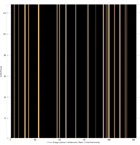
increased to 98 hits or 38.3% hit rate.

This plot allows one to identify, by regions with decreased slope, where the GA could

still use improvements. These low increase regions are common in the initial member, but the

final archive pushes most of these lower performing regions to the beginning and end of the CPI

indices. Given a moving platform that begins and ends at the edge of the ROI, this result is

expected as these points in the flight provide the greatest number of Azimuth angles, which can

miss the ROI. This information could also yield a more targeted mutation operator in the future.

It is also interesting to note that with only 38.3% of the CPIs falling within the region of interest,

the population is able to achieve a fitness of 0.88-0.91 in PSL and 0.82 -0.86 ISL, so perhaps the

(33)

[image:33.612.136.276.529.674.2] [image:33.612.330.471.531.679.2]

Figure 25.Initial VPH for the center cell of the ROI Figure 26. Final VPH for the center cell of the ROI

0 50 100 150 200 250 300 350 400 450 500 0

0.2 0.4 0.6 0.8 1

F

it

n

e

s

P

e

rf

o

rm

a

n

c

e

Generation

PSL Fitness ISL Fitness

0 0.1 0.2 0.3 0.4 0.5 0.6 0.7 0.8 0.9 1 0

0.1 0.2 0.3 0.4 0.5 0.6 0.7 0.8 0.9 1

In

te

g

ra

te

d

S

id

e

L

o

b

e

(34)

29

Figure 27. Initial 2D IFFT Normalized Magnitude Figure 28. Final 2D IFFT Normalized Magnitude

Figure 29. ROI Illumination per CPI

14.SAR MPI Scenario 45m by 120m

Maintaining a similar computational burden to the previous simulations, a larger ROI of

120m in the cross range dimension was examined. A simulation time of 1.384 and a PRF of 369

achieved a single cross range column illumination by upping the pulses per CPI to two from the

single pulse used in all preceding scenarios.

0 50 100 150 200 250 300

0 10 20 30 40 50 60 70 80 90 100

Coherent Pulse Interval (CPI)

T

o

ta

l

Il

lu

m

in

a

ti

n

g

P

u

ls

e

s

(35)

[image:35.612.197.411.103.641.2]

No. of Apertures 1

Bandwidth 50 MHz

PRF 369 Hz

No. of pulses 2

IFFT size 256 x 512

Beamwidth 5°

Range size 120 m

Range size 45 m

Interest 500 m

Azimuth angle

-31° to 31° in 32 steps

Objective Functions

Revisit & Pulse

Timing

Crossover Operator

Uniform 50%

0 0.1 0.2 0.3 0.4 0.5 0.6 0.7 0.8 0.9 1 0

0.1 0.2 0.3 0.4 0.5 0.6 0.7 0.8 0.9 1

In

te

g

ra

te

d

S

id

e

L

o

b

e

(36)

[image:36.612.106.257.412.562.2]

31 Figure 31. SAR Maximum Member Fitness Improvement

Figures 30 and 31 show that this scenario configuration experienced results consistent

with the previous experiments. PSL initially starting with a lower performance was rapidly

improved to an average fitness of 0.9 and ISL improved to 0.88. Examining the VPH and IFFT's

for the center cell also reinforced that when constrained to the same illumination per CPI, the

results are similar despite changes to the scenario time and ROI length.

Figure 32. Initial VPH for the center cell of the ROI 33. Final VPH for the center cell of the ROI.

0 50 100 150 200 250 20 40 60 80 100 120

D

o

w

n

R

a

n

g

e

Cross Range (Yellow = Illuminated, Black = Not Illuminated) 0 50 100 150 200 250

20 40 60 80 100 120

D

o

w

n

R

a

n

g

e

(37)

32

15.SAR 45m by 60m with 4 Apertures

This scenario is the first to utilize multiple sub-apertures and apply them to a ROI of 45m

by 60m. With the exception of the sub-apertures, the scenario is identical to section 14, running

for 0.692 seconds with a VPH size of 128 by 256. This run time allows the target platform to

traverse the length of the 60m ROI. Each CPI sub-aperture is allocated 12.5 MHz, or one quarter

of the down range resolution (32 cells), and one column in the cross range dimension. This

allocation of bandwidth yields VPH illumination patterns that are no longer symmetrical about

(38)

[image:38.612.196.411.104.642.2]

33 Table 8. SAR 45m by 60m with 4 Aperutres Parameters

No. of Apertures 4

Bandwidth 50 MHz

PRF 369 Hz

No. of pulses 1

IFFT size 256 x 512

Beamwidth 5°

Range size 60 m

Range size 45 m

Interest 500 m

Azimuth angle

-30° to 30° in 32 steps

Objective Functions

Revisit & Pulse

Timing

Crossover Operator

Uniform 50%

0 0.1 0.2 0.3 0.4 0.5 0.6 0.7 0.8 0.9 1 0

0.1 0.2 0.3 0.4 0.5 0.6 0.7 0.8 0.9 1

In

te

g

ra

te

d

S

id

e

L

o

b

e

(39)

[image:39.612.196.410.82.252.2] [image:39.612.321.515.299.459.2]

Figure 38. Initial VPH for the center cell of the ROI Figure 39. Final VPH for the center cell of the ROI

D o w n R a n g e

50 100 150 200 250

20 40 60 80 100 120

D o w n R a n g e

50 100 150 200 250

[image:39.612.90.285.300.457.2] [image:39.612.88.293.507.660.2] [image:39.612.318.527.508.661.2]

(40)

35 The results from this scenario offered a significant departure from the previous

simulations. Initial ISL performance shown in Figure 36, was comparable to the results in

section 14, starting with a fitness value of 0.6. PSL, which previously began lower then ISL,

found an initial value of 0.8, which was well above the expected ~0.48 fitness. One can see in

Figure 37 that PSL performance rocketed to saturation by the 50th generation, while the ISL only

managed to gain ~0.1 for a final archive fitness 0.7.

Comparing against previous sub-aperture work [1], one can see that this PSL and ISL

tradeoff is the anticipated result of introducing multiple sub-apertures. This simulation

reinforces the rapid improvement in PSL that can be achieved at the cost of ISL performance.

Further investigation should target whether the saturation of PSL fitness prevents further growth

in the ISL dimension. A new fitness map for the PSL function would also allow for one to

determine the maximum achievable PSL dB value, as the members in this simulation were not

rewarded for performance beyond the 14dB value seen in Figure 41.

16.SAR 45m by 1000m

This scenario is an attempt at running the SAR optimization on a ROI with the

dimensions used for the MTI mission. The cross range ROI size was increased to 1000 meters

and the scenario run time was set to 7.6293 seconds to allow the platform to fully traverse the

ROI. Instead of a -30° to 30° Azimuth angle, the genetic algorithm was set to optimize for

values between -60° and 60°. PRF was increased to 530 Hz, but the number of pulses per CPI

(41)

[image:41.612.203.412.92.497.2]

No. of Apertures 1

Bandwidth 50 MHz

PRF 530 Hz

No. of pulses 16

IFFT size 256 x 512

Beamwidth 5°

Range size 1000 m

Range size 45 m

Interest 500 m

Azimuth angle

-60° to 60° in 32 steps

Objective Functions

Revisit & Pulse

Timing

Crossover Operator

Uniform 50%

Based on the results of the previous experiments, one would have expected similar

performance of the PSL and ISL as each CPI is again illuminating a single cross-range column.

Although this scenario was only run for 300 generations versus the 500 of the pervious

simulations, both the initial and final fitness proved to be lower than expected.

One can see in Figure 43, initial PSL performance fell from a fitness of 0.6 to 0.36,

almost a 50% falloff compared to the 45m by 120m scenario. ISL also dropped to 0.59 from a

typical start of ~0.63. This starting deficiency was compounded by reduced performance

improvement across all generations of the scenario. Figure 42 shows that while PSL improved

by ~0.3 in the smaller scenarios, here it only experienced 0.1 fitness growth over the course of its

(42)

37 scenarios, was even slow to improve. ISL only gains 0.05 fitness in this 1000m scenario, which

[image:42.612.196.410.248.417.2]

is half the performance of the 120m scenario. One can see the small improvement between

Figure 44 and Figure 45; this cell has only gained a small amount of illumination after the 300

generations have run their course.

This scenario baselines the SAR performance in a large scale scenario so that it can be

compared against the large combined SAR/MTI mission, as well as combined with multiple

sub-aperture missions. Performance would likely be improved by tweaking the pulse per CPI, PRF

[image:42.612.197.411.464.633.2]

and CR VPH resolution parameters.

0 50 100 150 200 250 300

0 0.2 0.4 0.6 0.8 1 F it n e s s P e rf o rm a n c e Generation PSL Fitness ISL Fitness

(43)

[image:43.612.321.516.82.242.2]

38

Figure 44. Initial VPH for the center cell of the ROI Figure 45. Final VPH for the center cell of the ROI

17.SAR & MTI 45m by 1000m

This scenario combines the SAR and MTI missions for a 4-dimensional SPEA2

optimization run. It uses 2 dynamic parameters encoded into each CPI, the number of pulses and

the angle from -60° to 60°. The combination of a simultaneous SAR and MTI mission, as well

as running a SAR mission with a SPEA2 driven number of pulses were both novel to this

scenario. The dynamic pulse number was required as it is a crucial part of the fitness metrics

used for the MTI mission.

D

o

w

n

R

a

n

g

e

50 100 150 200 250

20 40 60 80 100 120

D

o

w

n

R

a

n

g

e

50 100 150 200 250

[image:43.612.87.287.82.238.2] [image:43.612.87.294.290.443.2]

(44)

[image:44.612.198.415.92.504.2]

39 Table 10. SAR and MTI Parameters

No. of Apertures 1

Bandwidth 50 MHz

PRF 369 Hz

No. of pulses 1, 8, 16, 32

IFFT size 256 x 512

Beamwidth 5°

Range size 1000 m

Range size 30 m

Interest 500 m

Azimuth angle

-60° to 60° in 32 steps

Objective Functions

Revisit & Pulse

Timing

Crossover Operator

Uniform 50%

Unfortunately, the addition of the MTI mission did not provide any benefit to the SAR

mission when comparing against the pervious scenario. Initial ISL and PSL performance was

equivalent with 0.59 and 0.37, respectively. Fitness growth across the 500 generations was weak

even when compared to the results of the previous 1000m SAR scenario. PSL and ISL both

grew by ~0.04; a very marginal improvement.

The MTI fitness metrics performed differently from the expectations set by the previous

stand-alone run. Revisit time increased its initial starting value from 0.7 to ~0.9, while Pulse

fitness fell from 0.6 to 0.5. The revisit time fitness was able to reach saturation, as it did in the

(45)

40 one can see that the pareto-optimal front was not the clean band previously observed in the MTI

mission. The diffusion is likely a result of now optimizing across the 4 fitness function.

[image:45.612.197.409.124.293.2]

Figure 49. MTI Fitness Improvement per Generation

0 50 100 150 200 250 300 350 400 450 500 0

0.2 0.4 0.6 0.8 1

F

it

n

e

s

P

e

rf

o

rm

a

n

c

e

Generation

PSL Fitness ISL Fitness

0 50 100 150 200 250 300 350 400 450 500 0

0.2 0.4 0.6 0.8 1

F

it

n

e

s

P

e

rf

o

rm

a

n

c

e

Generation

(46)

Figure 51. MTI Maximum Member Fitness Improvement

18.SAR & MTI 45m by 1000m 4 Apertures

This scenario combines all the previous investigations to produce a waveform controlling

4 sub-apertures across a 7.6293 second scenario. The algorithm is run with both the SAR and

MTI fitness functions for 500 generations.

0 0.1 0.2 0.3 0.4 0.5 0.6 0.7 0.8 0.9 1 0

0.1 0.2 0.3 0.4 0.5 0.6 0.7 0.8 0.9 1

P

S

L

F

it

n

e

s

ISL Time Fitness Initial Population

0 0.1 0.2 0.3 0.4 0.5 0.6 0.7 0.8 0.9 1 0

0.1 0.2 0.3 0.4 0.5 0.6 0.7 0.8 0.9 1

P

u

ls

e

F

it

n

e

s

Revisit Time Fitness Initial Population

(47)

Figure 53. MTI Fitness Improvement per Generation

0 50 100 150 200 250 300 350 400 450 500 0

0.2 0.4 0.6 0.8 1

F

it

n

e

s

P

e

rf

o

rm

a

n

c

e

Generation

Maximum Revisit Time Fitness Maximum Pulse Fitness

0 50 100 150 200 250 300 350 400 450 500 0

0.2 0.4 0.6 0.8 1

F

it

n

e

s

P

e

rf

o

rm

a

n

c

e

Generation

Multi-mission radar waveform design via a distributed SPEA2 genetic algorithm

RIT Scholar Works

Multi-mission radar waveform design via a

distributed SPEA2 genetic algorithm

Contents