Optimisation of condition number for eigenstructure problems

(1)

City, University of London Institutional Repository

Citation

:

Sayyad, Ali (2016). Optimisation of condition number for eigenstructure problems. (Unpublished Doctoral thesis, City, University of London)

This is the accepted version of the paper.

This version of the publication may differ from the final published

version.

Permanent repository link: http://openaccess.city.ac.uk/17326/

Link to published version

:

Copyright and reuse:

City Research Online aims to make research

outputs of City, University of London available to a wider audience.

Copyright and Moral Rights remain with the author(s) and/or copyright

holders. URLs from City Research Online may be freely distributed and

linked to.

City Research Online: http://openaccess.city.ac.uk/ [email protected]

(2)

OPTIMISATION OF CONDITION

NUMBER FOR EIGENSTRUCTURE

PROBLEMS

By

Ali A. Sayyad

A THESIS SUBMITTED FOR THE DEGREE OF DOCTOR OF PHILOSOPHY

CITY, UNIVERSITY OF LONDON

SCHOOL OF MATHEMATICS, COMPUTER SCIENCE AND ENGINEERING DEPARTMENT OF ELECTRICAL AND ELECTRONIC ENGINEERING

SYSTEMS & CONTROL RESEARCH CENTRE NORTHAMPTON SQUARE, LONDON EC1V 0HB

UNITED KINGDOM SEPTEMBER 2016

(3)

i

(4)

ii

Abstract

(5)

iii

(6)

iv

B

... 87

5.3 Algebraic characterization of Controllability Subspaces ... 92

5.3.1 Problem statement ... 93

5.3.2 Minimal dimension Controllability Subspaces ... 96

5.4 Assignability of the spectrum of a Controllability subspace ... 99

5.4.2 Assigning the spectrum of a Controllability Subspace ... 100

5.4.3 Eigenvalue placement algorithm based on mobility of open to closed loop spectra ... 104

5.4.4 Numerical example ... 107

5.5 Selection of the most orthogonal eigenvectors and sensitivity of closed-loop system based on the open loop – closed loop spectra method ... 112

6 Measurement of angle between subspaces in direct sum decomposition... 116

6.2 Problem statement and preliminary results ... 117

6.3 Measuring the degree of orthogonality ... 120

6.3.1 The Gramian ... 120

6.3.2 Condition Number ... 124

6.3.3 The Spread of Singular Values ... 129

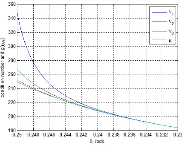
6.4 Numerical example ... 133

(9)

vii

7 Parameterisation of ordered minimal bases of Controllability Subspaces ... 139

7.2 Implicit system description ... 140

7.2.1 Duality issues and behavior ... 143

7.2.2 Computation of Input- State generator pairs Problem statement ... 147

7.2.3 Closed-loop Eigenvectors and frequency transmission ... 148

7.2.4 Pole assignment by output feedback and closed-loop Eigenvectors ... 149

7.2.5 Poles and Zeros ... 152

7.2.6 Design of state feedback controllers using Eigenvector parametrisation . 154 7.2.7 Selection of an independent Eigenframe and resulting state feedback ... 156

7.2.8 Parametrisation of ordered minimal bases and the selection of Eigenframes ... 159

8 Minimsation of the angle between closed-loop Eigenvectors via non- smooth Algorithm ... 172

8.2 Non-smooth optimisiation problem definitions ... 174

8.3 Generalized gradient of ... 176

8.3.1 ... 176

8.3.2 with ... 178

8.4 Smoothing approximation ... 180

8.5 Non-smooth Optimization Algorithm ... 182

8.6 Numerical examples ... 185

9 Conclusion and Future Research ... 193

9.1 Achievements, Results ... 193

9.2 Future Research ... 198

References... 201

Appendix_1 ... 209

( ( ))A x

κ

( )A

κ

( ( ))A x

(10)

viii

Acknowledgements

I would like to express my utmost gratitude to my supervisors Professor Karcanias and Professor Halikias.

Professor Karcanias who has been a most inspiring, yet demanding supervisor with a great insights in the field of Control Design Theory which have been invaluable during the work of this thesis. His constant support and guidance during my time of research have been priceless and have made this present thesis possible.

I would like also to thank Professor Halikias for his tremendous support and assistance in various sections of this thesis. His outstanding knowledge in both theory and programming aspects enabled me to achieve desired results throughout the time of research.

Finally, I would like to thank my family, Maryam and Diba, for their unconditional love, support and encouragement all these years. This thesis is dedicated to them for helping be what I am today.

(11)

1

CHAPTER 1 INTRODUCTION

1.1. Introduction

The purpose of this thesis is to study the problem of eigenstructure assignment in control systems design. This is achieved via a new methodology which relies on the minimisation of the skewness of the eigenframe of the state matrix. This reduces the sensitivity of the system’s eigenvalues to model perturbations and has as a result improvement of robustness of the system. The problem of eigenstructure assignment has a long history going back to the works done in 1975 [40], [98], [99].

Despite considerable work in this area, a number of fundamental issues still remain open and a number of key problems have not been properly addressed. In this work, the main emphasis has been on defining frames which are as orthogonal as possible. This guarantees minimal eigenvalue sensitivity due to a classical result by Wilkinson [1], applicable to the case of real distinct eigenvalues. The result in [6] has been the main motivation behind the minimisation of sensitivity of eigenvalues to parametric uncertainty.

(12)

2

insensitivity of the eigenvalues of the (closed-loop) state matrix is a highly desirable property of the feedback system since it can provide robust stability and robust performance properties to the design, i.e. avoiding loss of stability of performance characteristics due to the effects of model uncertainty.

The overall area of research in this field may be grouped to a number of areas, where particular aspects of the problem are considered. We may distinguish:

Problem Area I - System Properties and Eigen-frames: This area is crucial for design and relates to the problem of distribution, selection of poles and eigenstructure and overall system performance. Robustness, seen in a partial way, has been the dominant driving force in recent works done in the area of control.

Problem Area II - Parameterization of Eigen-frames: Additional work is needed in providing alternative descriptions that may be suitable for addressing different design issues. Evaluation of existing parameterizations, Minimal bases parameterisation of eigen-structures, Open-closed loop spectra parameterisation and related topics belong to this area.

Problem Area III - Design of Compensation Schemes for Achieving Desired Frame Spectrum: The design of compensation schemes involves the selection of

spectra and eigen-frames which satisfy certain criteria and their realization via specific feedback scheme configurations. In particular the following two problems can be distinguished:

(i) Selection of Eigen-frames

(ii) Feedback Realisation of Selected Eigen-frames

The key issue in the first area is the development of measures for orthogonality and other properties of eigenframes and then the definition of appropriate optimization problems that can produce the “best” - in some sense - frames.

(13)

3

the nature of optimal solutions and the feasibility of their realisation depends on the properties of the system model on which the various problems are posed. Investigating the links between system model and its potential for a design solution is the subject of the work here.

The essence of the work is to use this knowledge at the stage of design, redesign of system model, when there is the possibility to enhance the potential of the model to deliver solutions for multi objective and multi constraint type problems.

The above four areas are strongly interrelated. Note that most of the work so far has been in areas (II), (III), some in (I), but little in (IV) [3]. Within the current research and from the above problem areas, various problems related to the orthogonality of eigen-frames and robustness have been studied. These include the optimal choice of eigen-frames [6] which guarantees minimal eigenvalue sensitivity via a generalization of a classical result by Wilkinson [1], the definition of appropriate measures of “skewness” and the optimal choice of controllability subspaces in a standard direct sum decomposition using matrix fraction description (MFD).

This present research aims to develop a new methodology for determining the best angle between closed-loop eigenframes by computing the minimal condition number of the closed-loop eigenvector matrix. The importance of this methodology can be expressed in terms of results related to the Sensitivity of eigenvalues, Relative measures of controllability and observability and also deviations from strong stability to overshooting behaviour.

1.2. Objectives

Our main focus within this presented thesis has boon on the following objectives: Objective (1): Review ExistingMethodologies for Eigenstructure Assignment.

Objective (2): Develop Eigenstructure Parameterisations suitable for Eigenstructure Assignment.

(14)

4

Objective (4): Develop optimisation algorithms for selection of the most orthogonal frame and consider the influence of selected closed-loop spectra in such optimisations.

In fact, similar to any other research, we first will review some of existing methodologies around Eigenstructure assignment in order to explore the fundamentals and also to evaluate their pros and cons.

Among this variety of eigenstructure assignments and within this current research, the main attention has been paid to method introduced by Prof. Karcanias [4]. He first presents an alternative solution to the assignability of spectrum of controllability subspaces (cs) based on an eigenvector approach and then a new pole assignment algorithm has been derived as a practical application of this approach. In order to tackle the second objective, we then have developed a parametrisation on the closed- loop eigenvectors obtained from the method in [4]. The purpose here is to then work on this parametrisation and to improve the stability of the closed-loop control system with the direct attention to the condition number of the closed-loop eigenvector matrix. This in fact will result in a better closed-loop system performance based on the fact that the overall sensitivity of the system or the skewness of closed-loop eigenframes is minimized.

In general, the problem that frequently emerges in the study of performances of linear systems is the issue of “skewness” of eigenframes. This problem is linked to sensitivity of eigenvalues to parameter uncertainty, perturbations, as well as sensitivity of Nyquist diagrams to model parameter uncertainty. These skewness properties are also linked to measures of controllability and observability, when these are assessed in their model setting.

(15)

5

Consequently, prior to determination of objective Two, we have addressed a general problem of development of measures of “skewness” between subspaces, defined via a direct sum decomposition of the state space and by developing the concept of angle between subspaces. Three measurement tools have been applied in order to develop desirable outcomes for this objective. These tools are: Condition Number, Determinant of Gram Matrix and Singular Value Decomposition (SVD). Using these measurement tools, the objective is to derive necessary and sufficient conditions in each case, such that, the overall angle between subspaces in a direct sum decomposition is minimised.

Finally, the last objective will be to select the most orthogonal closed-loop eigenframe through development of a non-smooth optimisation algorithm and so considering the impact of selected closed-loop spectra in such optimisations. In fact, the problem will be to use one of those measurement tools applied to previous objective and generate the most orthogonal closed-loop eigenvector matrix such that error is minimised.

1.3. Main achievements

This thesis provides a structured and powerful new approach based on the results from Geometric Theory [5], [100], [101] which is an alternative to the work of Kaustky et al., [6], on the problem of perturbation of the eigenvalues and corresponding eigenvectors, by optimizing the condition number of the closed-loop eigenvector matrix.

The main achievement of the thesis is the development of a closed-loop eigenframe based on the following main principles:

i. A parameterisation of controllability subspaces (cs) leads to a family of direct sum decompositions of the state space.

(16)

6

iii. Define measures for the skewness of direct sum decompositions of the state space.

iv. Develop necessary conditions for minimising the skewness of the direct sum decomposition of the state space and algorithms for selection of the most orthogonal set of closed-loop eigenvectors in a cs.

In fact controllability subspaces are (A, B)-invariant subspaces with the property that any two points may be connected by some appropriate trajectory generated by a control input such that the trajectory always remains in the given space [9]. Their spectra are not fixed, and so the question arises as to whether or not such subspaces may assume any given spectrum. An alternative to the solution, already established based on an eigenvector approach, [10], is proposed here and involves the construction of characteristic bases having as a spectrum the set of assignable frequencies. We, however, have focused on the alternative parameterisation of eigenframes, [4], based on the property that such frames are arbitrarily assignable spectra that are characteristic bases of controllability subspaces, where we are searching for stabilisation, rather than exact eigenvector selection based only on frequency assignment.

Then, by defining and using three measurement tools which have been introduced earlier during this chapter, we have provided detailed and necessary conditions for the skewness of direct sum decompositions of the state space to be minimised. Finally, a non-smooth optimisation algorithm has been developed in order to select the most orthogonal set of closed-loop eigenvectors in a cs. Numerical examples have been presented in order for accuracy of the results to be tested where it has been necessary. The selection of the most appropriate stable spectrum leading to optimization of the orthogonality of the eigenframe has been considered for small dimension systems and the development of a procedure for the general dimension case remains an open question.

1.4. Summary of upcoming chapters

(17)

7

Chapter Two shall give a brief account of some of the mathematical and control topics which will be required in the reminder of this present research. Through its mathematical section, the definitions and/or theorems corresponding to some key concepts such as Condition number, Gram matrix, Singular value decomposition, Jordan Block, Vandermond matrix, etc are presented and proofed whenever it is strongly linked to the practical techniques which are used subsequently. The same work has been also done on some control-related fundamentals which are well connected to our main objectives of this presented thesis. These elements include Matrix Fraction Description (MFD), Minimal Bases of Matrix Pencils and their structures. These will lead to the study of controllability subspaces, which includes the important topic of matrix parameterisation of controllability subspaces through later chapters.

Chapter Three contains the literature review on Eigenstructure assignment including the relative basic concepts and background results. Throughout this chapter, a brief review of the concept of eigenvalues and eignevectors and their corresponding theorems is given. Then by reviewing the link between closed-loop eigenvalues and feedback, the problem of eigenstructure assignment has been reminded and reviewed through state and output feedbacks. Then some of main results achieved around state and output feedbacks have been presented including parametric cases.

(18)

8

eigenstructure assignmnets in order for a reader to obtain some more useful information around this subject.

Chapter Four presents the concepts of A- and (A,B) –invariant subspaces, followed by the construction and the existence of controllability subspaces connected to (A,B)-invariant subspaces. Through this chapter and from the geometric theory’s point of view, firstly the motion of eigenvectors within an A- invariant subspace of a linear system is reviewed and then by extending this matter to the (A,B)-invaraint subspaces, the Rectilinear motion of Nonautonomous system in the input output and state spaces is studied and presented. This will follow by the study of link between Simple Rectilinear Motion and one or R-dimensional (A,B)- invariant subspaces. Finally the concept of controllability subspaces is discussed in depth as the result of characteristic decomposition of (A,B)- invariant subspaces.

Within Chapter Five, the problem of eigenvector frame parameterisations is considered via two different parameterisations: first is the parameterization of closed-loop eigenframes based on the open and closed loop spectra and the second is based on the algebraic characterization and parameterization of controllability subspaces. These methods are in fact produced by Prof. Karcanias, [4], through his tremendous works done on the area of control system design theory.

Through this chapter, the relative fundamentals of each method are well-explained and then by introducing the Minimal Dimension Controllability Subspaces, assigning the spectrum of a controllability subspace is discussed and reviewed. This is then led to the Eigenvalue Placement algorithm based on mobility of Open to Closed Loop Spectra introduced by Prof. Karcanias [4].

(19)

9

Chapter Eight where this problem has been tackled and solved by a non-smooth optimisation method.

Chapter Six contains one of the main topics of this research: This is the problem of minimising the angle between subspaces in a direct sum decomposition which will be used in order to obtain the solution for the optimisation problem introduced at the final part of Chapter Five. During this chapter we tend to overview the issue of “skewness” of eigenframs in general which is linked to sensitivity of eigenvalues to parameter uncertainty, perturbations, as well as sensitivity of Nyquist diagrams to model parameter uncertainty. The objective of this chapter is to develop some measures of “skewness” between subspaces defining a direct sum decomposition of the state space and thus develop a concept of angle between these sets of subspaces. In fact our main aim in this chapter is to provide the required new concept of the relative positioning between subspaces that can be used in quantifying Sensitivity of eigenvalues as well as Relative measures of controllability and observability and also Deviations from strong stability to overshooting behaviour and for this purpose we will use The Gramian (determinant to be maximized), The Condition number (to be minimized ) and The Spread of singular values or a deviation measure of the singular values (which is minimized), as our three measurement tools. In this chapter we will proof that no matter which measurement is used, in all these cases the optimal condition arises when orthogonality conditions apply. The theoretical results are also supported by a number of numerical examples.

Chapter Seven presents an algebraic description of the total system behaviour which allows the study of closed loop eigenvectors in a systematic way by providing new parameterisations. This will then leads to an algebraic characterisation of the total input, state and output behaviour in an implicit formulation and it is given based on properties of MFD descriptions which will remain open for future studies.

(20)

10

impact of pole assignment using output feedback on closed-loop eigenvectors, this time via MFD’s. This will follow by a brief review of the link between system frequency and poles and zeros of the system since each of these is strongly link to the overall behaviour of the system. We then introduce new route for designing of State Feedback Controllers by using Eigenvector parametrisation and through ordered minimal bases, [33], [7], as the use of minimal bases suggests a simple procedure for selection of an independent eigenframe.

In fact in this chapter, the selection of the full rank eigenframe and its relation to the definition of state feedback along with the problem of minimal basis parameterization and its role to the shaping of frames are considered and deeply reviewed. This comes from the fact that each full rank closed-loop eigenframe can be written as the product of a matrix of ordered minimal bases (of matrix pencil) and a matrix containing all the existing eignevalues of the system in the form of Vandermonde matrix. As one can see, the matrix of ordered minimal bases has such importance as this is used to produce the controllability subspaces of closed-loop system and so if the optimal matrix is chosen then the stability of the system is guaranteed. This factor has led to the parametrisation of these minimal bases which is presented towards the end of Chapter Seven via Toeplitz form. In fact by exploiting the general parameterisation of the minimal bases, the general formula for any other minimal bases with the same degree can be computed using a Toeplitz matrix construction and the controllability subspaces separated by the largest possible angles can be identified. In each case, the theoretical results are illustrated with a numerical example. One interesting topic could be to use this parametrization and find a best choice of minimal bases such that the angle between these bases and consequently between the resulted controllability subspaces is maximized.

(21)

11

Chapter Six to assign and to reduce the Sensitivity of closed-loop eigenvetors for any controllable system(s), such that the system is robust to any perturbation injected to the eigenvalues or their relative eigenvectors, i.e. the error is minimized. The development of a robust and efficient optimization algorithm needs further consideration due to the non-convex nature of the optimization problem.

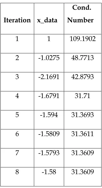
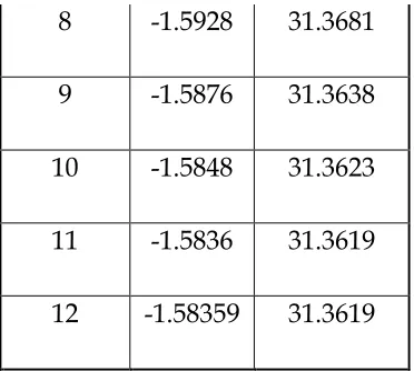
For this purpose, firstly, the concept of non-smooth optimisation has been derived [11]. Then by introducing the generalised gradient of condition number of any square symmetric matrix or its Gram matrix, the concepts of smoothing approximation following by non-smooth optimisation is described along with nay essential theorem and corresponding proof. Then by introducing an algorithm of relative optimisation method, our conditioning problem presented in Chapter Five is solved and some numerical results have been also derived.

(22)

12

CHAPTER 2 MATHEMATICS AND CONTROL

BACKGROUND

2.1. Introduction

In this section we give a brief account of some of the mathematical and control concepts which are required in future chapters of this work. Note that no attempt has been made to give complete proofs of all the fundamental theorems, unless these are strongly linked to the theory developed.

2.2. Mathematics background

2.2.1. Vector space.

This is a set

V

of vectors over a field

F

which is closed under the operation of addition (associative and commutative) and has an identity (

0) and additive inverse included within the set. The set is also closed under an operation of left multiplications of the vectors by any scalar of

F

with the following properties:

For a b, ∈F and x y, ∈V :

( ) ( )

a x y a x b y a b x a x bx a bx ab x ex x

+ = + + = +

= =

(23)

13

2.2.2. Subspace.

Let X be a nonempty subset of a vector space

V

over field

F

, that is: X ⊆

V

. If X is also a vector space over Field

F

for the same addition and multiplication operations, then X is called a subspace of

V

, i.e. if and only if:

,

x y∈X ⇒x+ ∈y X and

x∈X ⇒a x∈X for all a∈

F

. ([12], [14])

2.2.3. Orthogonal and Orthonormal vectors.

Let the angle

θ

between each two vectors of set of vectors 1, 2,...,

n k

x x x ∈ℂ is defined as:

cos

t i j t i j

x x x x

θ =

where

1

n t

i j i i i

x x x x

=

_∑

is the inner product of these two vectors. Then the whole set is

said to be a orthogonal set if θ =90Οor in other word x xt_i _j =0 where 1≤ ≤ ≤i j k. Additionally, these vectors are said to be orthonormal if each of them is normalized,

1

t i i

x x = , i=1,⋯,k. Note that an orthonormal set of vectors is linearly independent. [Refer to Horn and Johnson, 1985, Theorem 2.1.2, for complete proof]. ([12], [14], [15], [16], [17])

2.2.4. Unitary Matrix.

[12] A matrix U∈

M

n is said to be Unitary if and only if t

U U =I, where t

U is the conjugate transpose of matrix U .

2.2.5. Vector norm

s.

For any vectorx=[ ,x x1 2,⋯,xn] where ( )

n n

x∈ℂ orℝ , then the

p-norm of vector X is given by

1/

1 :

p n

p i p

i

x x

=

 

= 



∑

 where p≥1. For this vector

x

,

there are some very famous norms, which are used frequently and are defined as follow:

(i) Euclidean norm (2-norm), is defined as :

2 2

1

: _n

x = x + +⋯ x or

1/ 2 2 2

1 :

n i i

x x

=

 

=_ _

(24)

14 (ii) 1-norm , is represented as: ₁

1

:

n i i

x x

=

∑

(iii) ∞-norm (Maximum norm), is defined as:

1

: max( , , _n)

x_∞ = x ⋯ x ([12], [14], [17]).

2.2.6. Matrix norms.

Because m n×

ℂ is a vector space of dimensionm n. , magnitudes of matrices m n

A∈ℂ × can be “measured” by employing any vector norm on m n×

ℂ ([14]).

In this work the following two matrix norms are used ([12], [14], [15], [17]):

(i) Frobenius matrix norm is defined by

min( , )

2 ₂

1 1 1

( )

m n m n

t

ij i

F

i j i

A

α

trace A A

σ

= = =

≡

∑∑

= =

∑

where αij denotes any element of matrix A, t

A is the conjugate transpose of matrix A and

σ

i defines any singular values of A.

(ii) Matrix 2-norm

The matrix norm induced by the Euclidean norm is

2

max 2 max_X ₁ 2

A Ax

λ

=

= =

where

λ

maxis the largest eigenvalue such that

t

A A−λI is singular. In other words:

max

2 ( )

t

A =

λ

A A ,

t

A is the conjugate transpose of matrix A. (iii) Matrix 1-norm is defined as follow:

1

1 max_X ₁ 1 max_j ij

i

A Ax a

=

= =

∑

(25)

15

The matrix norm induced by vector ∞-norm is as follows:

1

max max _ij

X i

j

A Ax a

∞

∞ = ₌ ∞=

∑

.

i.e. the largest absolute row sum of a matrix.

2.2.7. Hadamard’s inequality theorem.

Let ( ,a a1 2,⋯,an)be columns (vectors)

in n

ℝ andA=( ,a a1 2,⋯,an)be the corresponding n n× matrix. The Hadamard’s

inequality states that:

1

det

n n n

A a

=

≤

∏

, where . is the Euclidean norms on vectors in n

ℝ . ([18], [19]).

2.2.8 .

Gramian (Gram) Matrix.

[17] Consider vectors 1, 2, ,

n n

x x ⋯ x ∈ℝ . The Gram matrix of the collection is the m m× matrixGwith elementsGij =x xti j. The matrix can

be expressed compactly in terms of the matrix X =[ ,x1 ⋯,xn], as

(

)

1

1 .

t t

m t

m

x

G X X x x

x     = =_ _    

⋮ ⋯

By construction, a Gram matrix is always symmetric, meaning that Gij =Gji, for

every pair ( , )i j . It is also positive semi-definite, meaning that u GuT ≥0, for every vector u∈ℝn (this comes from the identity u Gut = Gu 2₂).

Assume that each vector xi is normalized: xi ₂ =1. Then the coefficient Gij can be

expressed asG_ij =cosθ_ij, where θij is the angle between the vectors xi and xj.

Thus Gij is a measure of how similar xi and xj are ([12], [20]).

(26)

16

2.2.9. Condition Number.

For any n n× matrix A, the condition number

κ

(Α) ≥1,

based on matrix 2-norms, is defined to be : 1

.

A A

κ_{(Α) =} −

. Similarly, the condition number could be also defined using the singular values of matrix A as follows:

1( )

( )

n

A A

A

σ κ

σ

= where

σ

1is the largest and

σ

nis the smallest singular value of matrix

A([12], [21]).

A matrix is so called: “well-conditioned” if its value of condition number is low and is called to be “ill-conditioned” if its condition number is high.

2.2.10. Vandermonde matrix.

A n n× Vandermonde matrix A is a matrix of form

0 1

0

1 1 1

0 1

1 1 1

( , , _n) n

n n n

n

x x x

A A x x

x − x − x −

 

 

= =_ _

 

 

⋯ ⋯ ⋯

⋮ ⋮ ⋮

⋯

where x1,⋯,xn∈

F

, that is, A=  aij with

1

j ij i

a =x − . The determinant of this matrix can be computed as:

, 1

det( ) ( )

n

i j i j

i j

A x x

= >

=

∏

−

A is nonsingular if and only if all the parameters x1,⋯,xn∈

F

are distinct.

Note that the Vandermonde matrix evaluates a polynomial at a set of points; formally, it transforms coefficients of a polynomial 2 1

0 1 2 1

n n

a +a x+a x + +⋯ a ₋x − to the values the polynomial takes at the points α_i_{. The non-vanishing of the}

Vandermonde determinant for distinct points α_i_{shows that, for distinct points, the}

(27)

17

2.2.11. The Jordan Canonical Form of a Matrix.

For an n n× complex matrix A, there exists a non-singular matrix T such that 1

1

( , , _k),

T AT− = =J diag J ⋯ J where:

1 0

1

0 1

i i i

i

J

λ

 

 

=

 

 

⋱ ⋱ ⋱

ismi×mi and m1+ +⋯ mk =n. The matrices Ji are called Jordan matrices or Jordan

blocks, J is called the Jordan Canonical Form (JCF) of A and

λ

_i,i=1, 2,⋯, k is the eigenvalue of A with multiplicity of mi. The same eigenvalue can appear in more

than one block ([12], [17], [21]).

2.3. Control background

This part of the chapter describes a very important tool which is used to the study of controllability subspaces. This leads to one of the main topics of the current research which involves the best parameterization of the controllability subspaces in a direct sum decomposition in order to compute the minimal basis of the whole controllability space.

2.3.1. Matrix Fraction Description (MFD)

We first introduce the basics of MFD and then review the problem statement related to the controllability subspaces by studying some basic concepts and definitions. The first step when studying and designing a control strategy for a physical system is the development of mathematical equations that describe the system. The linear equations used to describe linear systems are generally limited either to:

- input-output description (external description) or

(28)

18

Prior to 1960, the design of control systems had been mostly carried out by using transfer functions. However, the design had been limited to the single variable, or single-input-single-output (SISO) case. Its extension to the multivariable, or multi-input-multi-output (MIMO) case had not been successful.

The state-variable approach was developed in the sixties, and a number of new results were established in the SISO and MIMO cases. At that time, these results were not available in the transfer-function, or polynomial approach, so the interest in this approach was renewed in the seventies. Now most of the results are available both in the state-space and polynomial settings. Refer to [2], [5], [8], [13] and [71] for some of these results.

2.3.1.1. Scalar systems

- Rational transfer function (RTF)

Although there are too many different interpretations related to Rational Transfer Function, here we will present the fundamental summary of RTF including major definitions and the way that RTF is constructed ([13], [23], [30]).

Assuming that the knowledge of the internal structure of the system is not available, the transfer function description of a system gives a mathematical relation between the input and output signals of the system.

Assuming zero initial conditions, the relationship between the input uand the output y of a system can be written as

( ) ( ) ( )

y s =G s u s

(29)

19

In the above description of a transfer function, it is assumed that polynomials n s( ) and d s( )are relatively prime. The degree of denominator polynomial d s( )is the order of the linear system.

Here we give some of useful definition relative to the matrix fraction description area:

Monic polynomial: The polynomial with leading coefficient equal to one ([13], [23], [30]).

Nominal transfer function: When the denominator polynomial is monic, then the transfer function is normalized or nominal ([97]).

Column-reduced: A polynomial matrix with non-singular column leading coefficient matrix ([13], [23], [30]).

Greatest common divisor: A highest degree common factor that can be extracted from two polynomials ([13], [23], [30]).

Hermite form: A triangular canonical form of a polynomial matrix ([13]).

Irreducible: A transfer function is irreducible when its numerator and denominator polynomials are relatively prime ([13], [23], [30]).

Leading coefficient matrix: The constant matrix whose entries are built from coefficients of highest powers of the entries of a polynomial matrix ([13], [23]).

Left MFD: An MFD where the denominator polynomial matrix enters from the left ([13], [23], [30]).

Matrix fraction description: Ratio of two polynomial matrices describing a matrix transfer function ([13], [23], [30]).

Minimal: A state-space realization is minimal if it has the lowest possible dimension ([13], [23])

(30)

20

polynomial. If the degree is greater, then the transfer function called the strictly proper ([13], [23], [30]).

Rational vector space: The linear vector space over ℝ( )s contains all the rational functions in s having real coefficients (∈ℝm n× ( )s ) ([33]).

Relatively prime: Two polynomials or polynomial matrices are relatively prime if they have no common factor ([13], [23], [30]).

Right MFD: An MFD where the denominator polynomial matrix enters from the right ([7], ([13], [23], [30]).

Row-reduced: A polynomial matrix with non-singular row leading coefficient matrix ([13]).

Unimodular: A polynomial matrix with a non-zero constant determinant ([13], [23], [30]).

For a system:

,

E xɺ=Ax+Bu y=C x

with n variables, m inputs, and p outputs, the transfer function 1

( ) ( )

G s =C sE−A − B is a p×m matrix whose elements are rational functions.

A closer analogy to the SISO case is the matrix fraction description:

1 1

( ) _R( ) _R ( ) or ( ) _L ( ) _L( )

G s =N s D− s G s =D− s N s whereN_R,D N_R, _L,D_L are polynomial.

We can define a right matrix fraction description, or right MFD for short, 1

( ) _R( ) _R ( )

G s =N s D− s

Alternatively, we can also define a left MFD 1

( )G s DL ( )s NL( )s −

(31)

21

It is always possible to go from right MFD’s to the left and vice versa.

There can be many right and left matrix fraction description (MFDs) of G s( ). Indeed, given a right MFD, an infinity of others can be obtained by choosing any

non-singular polynomial matrix U s( )such that:

( ) ( ) ( ), ( ) ( ) ( )

R R R R

N s =N s U s D s =D s U s .

We call U s( ) a right divisor of N_R( ) and s D s_R( ). Moreover, since

deg det D (s) = deg detD (s)+deg detU(s)R R , it holds:

deg det D (s) _R ≥ deg detD (s)_R

which means that the degree of a MFD can be reduced by removing right divisors of the numerator and denominator matrices.

Obviously, we will get a minimum-degree right MFD by extracting a greatest common right divisor (gcrd) ofNR( ) and s D sR( ). In other words, a gcrd from NR( ) and s D sR( ) is

extracted if and only if deg det D (s) = deg detD (s)_R _R .

If N_R( ) and s D s_R( )have only unimodular right gcrds, then these two matrices are right

coprime and the right MFD 1

( ) R( ) R ( )

G s =N s D− s is irreducible. Similar statements can be given for left MFDs ([13], [23], [30]).

For every transfer function

( ) ( )

( )

n s G s

d s =

there is an unlimited number of state-space realizations. Some of them such as canonical realizations, known as the controllable and observable forms which are commonly used depend on the application and requirement.

If ( ) n p[ ]

(32)

22

Least degree basis: V s( )∈ℝn p× [ ]s is a least degree basis if the greatest common divisor of all its m m× minors is equal to 1 ([25]).

Minimal basis: The basis V s( )∈ℝn p× [ ]s is called minimal if it is row proper and it has least degree ([7], [33]).

The degree of V s( ): The degree d of the basis V s( )∈ℝn p× [ ]s is the highest degree among all the m m× minors of the matrix V s( ) ( [25], [33],).

The complexity of V s( ): ([13], [23], [30]). The complexity c of the basis V s( ) is the sum of the degrees of its row vectors, i.e..,

1

m i i

c δ

=

∑

.

Note that normallyc≥d, V s( ) is so called row-proper if and only if c=d. For any full rank polynomial matrix M s( )which is m×p m ( > p), we can create a module

M

_{, by multiplying from the right to a uni-modular matrix} Q s( ), p× p, and

( ) 0

Q s = ≠c , such that M s Q s( ) ( )=

M

_M( The degree of

M

M is the maximum degree

of C M s_p( ( )) where C M s_p( ( ))is the exterior product of minor p of M s( )).

So for any other bases M s'( )=M s Q s( ) ( ), the degree of M s( ) & M s'( ) is the same. If we introduce M s( ) to be:

1

( ) ( ), , _p( )

M s =_m s ⋯ m s _

and δ1,⋯,δp are the degrees of each row polynomial vector

1 0

( ) i i

i i i i i

m s =m sδ δ + +⋯ m s+m , where each i

i

mδ contains the coefficients related to the highest degree of its polynomial .

Denote vector i

i

mδ as mih; then the row highest coefficient matrix of M s( ) is the

matrix 1 2

h h h

p h

M =_m m ⋯ m _ which contains just the constants value and M s( )

(33)

23

1

2

1 2

0 ( )

0 p

h h h

p

s s

M s m m m

s

δ δ

δ

 

 

 

=_ _{ } _+

 

 

⋯ ⋯

⋱ .

Note that M s( ) is row proper if and only if, Mhis full rank. ([25])

2.3.2. Minimal bases of matrix pencils and coprime matrix descriptions

In this part, we review the problem of constructing coprime MFD’s from a minimal state space realization of a transfer function matrix. This part is widely used in the analysis and design of linear systems described by transfer function matrices using MFD’s. The main results in this section are taken from Karcanias (2002) [7], [8], [100].

Consider the minimal system described by

x Ax Bu

y Cx

= +

  ₌ 

ɺ

(2.3.1)

whereA∈ℝn n× ,B∈ℝn p× ,C∈ℝm n× and with transfer function matrixG s( )∈ℝm p× ( )s . The problem here is to find the right and left coprime MFD’s for G s( ), i.e. to express

( )

G s as :

1 1

( ) ( ) ( ) '( ) '( )

G s =N s D s − =D s − N s (2.3.2) where N s N s( ), '( )∈ℝm p× ( ), ( )s D s ∈ℝp p× ( ), '( )s D s ∈ℝm m× ( )s and (N(s),D(s))are right coprime and (D s N s'( ), '( ))are left coprime.

It can be shown [7] that the computation of coprime MFD’s from state space description is reduced to computation of coprime MFD’s of the transfer functions:

1 1

( ) ( ) , ( ) ( )

IS SO

(34)

24

It is evident that the above descriptions are dual and thus treatment of the first provides also solution for second. Let us consider H_IS( )s and right MFD’s, i.e.

1 1

(sI−A)− B=N s D s( ) ( )− [ , ] ( ) 0, ( ) ( )

( ) ( )

N s N s

sI A B T s

D s D s

   

⇒ − −  = = 

    (2.3.4)

Given that ( ( ),N s D s( )) is right coprime, from the full rank property of pencil

[

sI− −A B,

]

, we have the following results:

Proposition 2.1:Every least degree polynomial basis of:

{

,

}

, Z ( ) [ ( ) ; ( ) ]t t t

r sI− −A B r s = X s U s

N

, i.e. [ , ] ( ) 0

( )

X s sI A B

U s   − − _ _=

  (2.3.5)

Defines a right coprime MFD for H_IS( )s = 1

( ) ( )

N s D s − , where

( ) ( ), ( ) ( )

N s = X s D s =U s .

Proof: See [7] for full proof.

The above result stated for least degree base is also valid for minimal bases. If (( ) ) †

,

n p n p n

N∈ℝ − × B ∈ℝ × is a pair of left annihilator, left inverse of B(NB=0, rank rank N= −n p,B B† =Ip), then

†

( ) ( ) 0 ( ) ( ) ( )

sN NA X s

U s B sI A X s

− =

= − (2.3.6)

The pencil sN−NAhas(n− ×p) ndimension and its significance is emphasised by the following result.

Proposition 2.2: The pair (X s U s( ), ( ))defines a minimal basis Z s_r( ) for

{

[ , ]

}

r sI− −A B

N

_{, if and only if} X s( ) is a minimal basis for

N

_r[sN−NA]_{([7], see}

(35)

25

During next section, we will review the methodologies used to obtain the minimal bases of matrix pencil in more detail.

2.3.3 Construction of minimal bases of matrix pencils and coprime matrix fraction descriptions using Toeplitz matrix

Since coprime MFDs have been used widely in linear control theory, several methods for their computation have been developed ([7], [13]). A first approach was developed in Rosenbrock (1970) [26].

This method requires elementary row operation on polynomial matrices and is therefore difficult to implement on a computer and can be numerically unstable. There are two other main approaches that have emerged so far: the reduction to the block Hessenberg form (BHF) and the minimal design problem (MDP).

The BHF approach uses state space realisations starting from controllable realizations and then by suitable transformations that reduces to the Hessenberg form. In other words, the approach consists of a transformation from state space model S A B C D( , , , ) to reduced modelS F G H( , , )where the matrix F is the lower (upper) block Hessenberg matrix. Orthogonal transformations are preferred for the reduction to BHF because of their attractive numerical stability properties.

Reduction to the block Frobenius form (BFF) can also be employed, i.e. the model ( , , )

S F G H can be reduced to the formS F G H( , , ), where F is in BFF. By permutation of the state space variables of S F G H( , , ) a canonical representation

( _c, _c, _c)

S F G H similar to the Lueberger canonical form is obtained.

(36)

26

The main disadvantage of these methods is that they involve operations on matrices whose orders may often be much higher that the dimension of the state space of the given system.

Another method for obtaining relative prime MFD from a state space representation of the transfer function is given by Wolovich (1974) [30], [31]; Wolovich & Falb (1969) [32] and Datta & Gangopadhyay (1992) [28].

This method is most commonly used for computation MFD’s since it is the easiest to implement on a computer and can be used for high-order system. The disadvantage is that the state space system must first be transformed to the Lueberger canonical form which can be quite sensitive numerically.

Here we give two methods of computation of coprime MFD’s using Toeplitz matrix by Karcanias (2002) ([7], [96], [100]). These are the indirect and direct methods which are based on the construction of minimal bases for the kernels of the state-space-based pencils[sI− −A, B], [sI−At,−Ct].

2.3.3.1. Computation of minimal bases for

N

_r

{

[sI− −A B, ]

}

using the Toeplitz structure: the indirect method [7], [100]

First essentials notation and definitions are introduced:

For the pencil R s( )=sNA NA− =sF G− we first note the following:

If T s( )=[sI − −A, B] and R s( )=sNA NA− and Z andX respectively their rational, right null spaces respectively, then:

The ordered set of Forney dynamical indices [33] ofX , or column minimal

indices (cmi) of the corresponding pencils are denoted by:

{

1

}

( )= ( ,

ε ρ

_i _i),i∈

µ

, 0≤ ≤ ≤

ε

…

ε

_µ ɶ

I X

_(2.3.7)

{

1

}

( )= ( ,

ε ρ

ɶ ɶ_i _i),i∈

µ

, 0≤ ≤ ≤

ε

ɶ …

ε

ɶ_µ ɶ

(37)

27 Note that

ρ ρ

i = ɶi,

ε ε

ɶi = + ∀ ∈i 1, i

µ

ɶ . In the above,

ρ ρ

i, ɶi denote the multiplicity of the

distinct value of

ε ε

_i,ɶ_i. The

ε

ɶi are known as the controllability indices of the S A B( , )

system.

- Any minimal basis matrix of X , X s( ) is called an ordered minimal basis matrix (OMBM) if it may be expressed as :

1 1 0

( ) ( ); ; ( ) , ( ) i i[ ]

i

n

i i i

i

X s =_X s ⋯ X_µ s _ X s =s Xε _ε + +⋯ sX +X ∈ℝ ×ρ s (2.3.9) - If the Toeplitz matrix related to Xi for every k≥

ε

i with fi = − ≥k

ε

i 0,is as :

1

( 1) ( 1) 0 1 0 0 0 0 ( ) 0 0 0 i i i i i i i i

k n f k i i i i X X X T X X X X ε ρ ε ε + × +             =_ _∈             ⋯ ⋯ ⋮ ⋱ ⋮ ⋱ ⋮ ℝ ⋱ ⋱ ⋱ ⋮ ⋮ ⋱ ⋱ ⋯ ⋯ (2.3.10)

also known as the kth Toeplitz matrix of X s_i( ).

Then the kth Toeplitz matrix of ( , )F G pair is defined as:

( 2) ( 1)

0 0

( , )

0

0 0

k q k n k

F G F

G T F G

F G + × +   ₋     −  = ∈       −   ⋯ ⋯ ⋮ ℝ ⋮ ⋮ ⋱ ⋮ ⋱ ⋱ ⋯ ⋯

(38)

28

So above notations and results provide the means for the construction of special basis matrices k

r

N spaces, which in turn lead to the construction of minimal bases for space

N

_r

{

[sI− −A B, ]

}

.

Here is the indirect algorithm ([7], [96]):

Part (I): Computation ofI X( ). For all the k≥0 compute rankT_k( , )F G =

σ

k,

0,1, 2,

k= ⋯.

The right nullity of Tk( , )F G defined by rk = +(k 1)n−

σ

k,k =1, 2,⋯.This defines the

sequence

C

r( , )F G =

{

r kk: ≥ −2,r−2=r−1= ∀ ≥0, k 0

}

. By computing the gap sequence

2 2 1, 0, 2, 1 0

k rk rk rk k r r

δ

= + − − − ≥ − − = (2.3.12)

the distinct values of

ε

iare defined by those values of k for which

δ

k >0 and the

corresponding multiplicity

ρ

i is the value of

δ

k >0.

This defines ( )=

{

( ,

ε ρ

i i),i∈

µ

, 0≤ ≤ ≤

ε

1 …

ε

µ

}

ɶ

I X

_.

Part(II): Computation of a set of state generator ΩXI . Having

{

1

}

( )= ( ,

ε ρ

_i _i),i∈

µ

, 0≤ ≤ ≤

ε

…

ε

_µ ɶ

I X

the computation of a set

{

,

}

i

N_ε i

µ

Ω = ∈

ɶ

I X involves the following steps:

Step(1): Fork=

ε

1, compute any basis matrix for r1

ε

N _{and let this be} 1 1 1

( 1)n N_ε ∈ℝε+ ×ρ . Step(2):For k=

ε

2, compute

2 1 ( 1)

T_εε N_ε and complete it to a basis for 2

r

ε

N . This defines

2 2 2

( 1)n N_ε ∈ℝε + ×ρ .

Step(i) (General step): Let

{

}

1, , i1 N_ε N_ε

−

⋯ be the matrices defined by the previous step for k =

ε

i−1.For k=

ε

i compute ( ₁, , ₁)

i

Tε N_ε ⋯ N_ε₋ and complete it to a basis of i

r

ε

N . This defines (i 1) i

i

n

(39)

29

The procedure is completed in µ steps and this leads to a set of state generators

{

( 1)

}

, i i,

i i

n

N_ε N_ε ε+ ×ρ i

µ

Ω = ∈ℝ ∈

ɶ

I

X .

Part (III): Computation of the OMBM of X . Each of the matrices N_ε_iin 0

{

( 1)

}

, i i,

i i

n

N_ε N_ε ε+ ×ρ i

µ

Ω = ∈ℝ ∈

ɶ

I

X can be partitioned as shown below:

1

0

, , 0,1, , ,

i

i i

n i

j i

i i

X X

N X j i

X X

ε ε

ρ

ε ε µ

−

×

       

=_ _ ∈ ∀ = ∀ ∈

       

⋮ ℝ ⋯

ɶ

and thus we define the OMBM by:

1 1 0

( ) ( ); ; ( ) , ( ) i i[ ]

i

n

i i i

i

X s =_X s ⋯ X_µ s _ X s =s Xε _ε + +⋯ sX +X ∈ℝ ×ρ s .

2.3.3.2 Direct method for computing a minimal basis for the right null space

[sI− −A, B]

Opposite to the indirect method, in this method we will consider the direct method introduced by Karcanis in his published paper in 2002 [7], which although it involves larger dimension pencil, [sI− −A, B] instead of sN −NA, it has the more convenient form, which avoid Toeplitz matrix computation.

Let ( ( ), ( ))X s U s be a pair of polynomial matrices such that:

(sI−A X s) ( )=BU s( ) (2.3.13) whereX s( )∈ℝn q× ( ), ( )s U s ∈ℝp q× ( ),s and the scalar degree of U s( )is kand thus that of

( )

X s is k−1. We may call such pair as ( , )k q -order right pair and write them as 1

0 1 1

( ) k k k kk

X s =X +sX + +⋯ s − X ₋ (2.3.14) 1

0 1 1

( ) k k k _kk k _kk.

(40)

30

By substituting these two in equation (2.3.13), we will get the following equation

1 1 2 2 1 1 0 0 0 0 0 0

0 0 0

0.

0 0 0 0 0 0 0 k k k k k k k k k k k k k k U I X

A B I

U

A B I

X

U

X

U

A B I

X A B U − − − −     −  _{ } _  ₋ _{ } _  _{ } _  − _ _  _{ } _  _{ } _  _ _₌  _{ } _  _{ } _  _{ } _  _{ } _ −  _{ } _  _{ } _       ⋱ ⋱ ⋮ ⋱ (2.3.16)

=T A B_k( , ) =Z_k

The Toeplitz matrix T A B_k( , ) characterizes the minimal bases. This equation even can be made simpler which it has been made simplified during the work done by Karcanias (2002) [7]. By some more calculations he shows that the whole solution can be done in the easier way as the following proposition:

Proposition 2.3. A ( , )k q -order right pair of S A B( , ) , for which ρ( )B = p, described as:

1

0 1 1

( ) k k k kk

X s =X +sX + +⋯ s − X ₋ 1

0 1 1

( ) k k k _kk k _kk.

U s =U +sU + +⋯ s −U ₋ +s U is defined from the set

{

0, 1, ,

}

k k k

k

U U … U which is the solution of the equation

1 1

1

0

, , , , 0.

k k k k k k k k U U

A B A B AB B

U U − −           ₌  _{ } _      

… ⋮ (2.3.17)

(41)

31

Proof: Refer to [7] for full details.

For any solution of above equation the parameters 0, 1, , 1

k k k

k

X X X ₋

 

 … are defined by

1 2 1 1 2 3 1 2 1 2 0 1

0 0 0

ˆ 0 k k k k k k k k k k k k k k k k k B X U AB B U U X

A B A B B

U U

A B A B AB B

U U − − − − − − − −                     = =             _ _{ } _   ⋯ ⋯ ⋮ ⋮ ⋮ ⋮ ⋱ ⋮ ⋮ ⋮ ⋮ ⋯ ⋯

. (2.3.18)

=R A B_k( , )

The matrix that determines the overall solvability is the kth order controllability matrix of the system and it is defined by

1

( , ) k , k , , ,

k

Q A B =_A B A −B… AB B_

Here is the algorithm for finding OMBMs of Z :

Part (I): Computation ofI Z( ). For all the k≥0 compute rankq_k =Q A B_k( , ), 0,1, 2,

k= ⋯, and thus the sequence

{

2 1

}

( , ) : 2, ( , ), 0 and , 0 .

r A B qk k qk rank Q A Bk k q p q

∗

− −

= ∀ ≥ − = ∀ ≥ = =

C

By computing the gap sequence:

1 2

2 , 0

k qk qk qk k

δ

ɶ = − − − − ∀ ≥ (2.3.19)

the distinct values of

ε

ɶiare defined by those values of k for which

δ

ɶk >0 and the

corresponding multiplicity

ρ

i is the value of

δ

ɶk >0. This defines

{

1

}

( )= ( ,

ε ρ

_i _i),1≤ ≤ ≤

ε

_µ,i∈

µ

.

ɶ

ɶ ɶ … ɶ

ɶ

Optimisation of condition number for eigenstructure problems

City, University of London Institutional Repository

Citation

:

This is the accepted version of the paper.

This version of the publication may differ from the final published

version.

Permanent repository link: http://openaccess.city.ac.uk/17326/

Link to published version

:

Copyright and reuse:

City Research Online aims to make research

outputs of City, University of London available to a wider audience.

Copyright and Moral Rights remain with the author(s) and/or copyright

holders. URLs from City Research Online may be freely distributed and

linked to.

OPTIMISATION OF CONDITION

NUMBER FOR EIGENSTRUCTURE

PROBLEMS

By

Ali A. Sayyad

Abstract

Table of contents

B

Acknowledgements

CHAPTER 1

INTRODUCTION

1.1.

Introduction

1.2. Objectives

1.3. Main achievements

1.4. Summary of upcoming chapters

CHAPTER 2

MATHEMATICS AND CONTROL

BACKGROUND

2.1. Introduction

2.2. Mathematics background

2.2.1. Vector space.

V

F

F

2.2.2. Subspace.

V

F

V

F

V

F

2.2.3. Orthogonal and Orthonormal vectors.

θ

∑

2.2.4. Unitary Matrix.

M

2.2.5. Vector norm

s.

∑

x

∑

2.2.6. Matrix norms.

α

σ

∑∑

∑

σ

λ

λ

λ

∑

∑

2.2.7.

Hadamard’s inequality theorem.

∏

2.2.8

.

Gramian (Gram) Matrix.

(

)

2.2.9.

Condition Number.

κ

_∑