City, University of London Institutional Repository
Citation
:
Malgarinos, I., Nikolopoulos, N., Marengo, M., Antonini, C. and Gavaises, M. (2014). VOF simulations of the contact angle dynamics during the drop spreading: Standard models and a new wetting force model. Advances in Colloid and Interface Science, 212, pp. 1-20. doi: 10.1016/j.cis.2014.07.004This is the accepted version of the paper.
This version of the publication may differ from the final published
version.
Permanent repository link:
http://openaccess.city.ac.uk/13573/Link to published version
:
http://dx.doi.org/10.1016/j.cis.2014.07.004Copyright and reuse:
City Research Online aims to make research
outputs of City, University of London available to a wider audience.
Copyright and Moral Rights remain with the author(s) and/or copyright
holders. URLs from City Research Online may be freely distributed and
linked to.
City Research Online: http://openaccess.city.ac.uk/ [email protected]
VOF simulations of the contact angle dynamics during the drop
spreading: standard models and a new wetting force model.
Ilias Malgarinos1, Nikolaos Nikolopoulos1,5, Marco Marengo2,4, Carlo Antonini2,3 and Manolis Gavaises1
1: School of Engineering and Mathematical Sciences, City University London, Northampton Square, EC1V 0HB London, UK, *Corresp. Author – e-mail: [email protected]
2: Department of Engineering, University of Bergamo, viale Marconi 5, 24044 Dalmine, Italy
3: Laboratory of Thermodynamics in Emerging Technologies, Department of Mechanical and Process Engineering, ETH Zurich, Zurich 8092, Switzerland
4: School of Computing, Engineering and Mathematics, University of Brighton, Brighton BN2 4GJ, UK
5: Centre for Research and Technology Hellas, Chemical Process and Energy Resources Institute, Egialeias 52, Marousi, Athens, Gr-15125, Greece
Abstract
A novel numerical implementation for the adhesion of liquid droplets impacting normally on solid dry surfaces is presented; the physical model is implemented as a source term in the momentum equation of a Navier-Stokes CFD flow solver as an “adhesion-like” force which acts at the triple-phase contact line as a result of capillary interactions between the liquid drop and the solid substrate. The advantage of this new approach, compared to the majority of existing models, is that the dynamic contact angle forming during the surface wetting process is not inserted as a boundary condition, but is derived implicitly by the induced fluid flow characteristics (interface shape) and the adhesion physics of the gas-liquid-surface interface (triple line), starting only from the advancing and receding equilibrium contact angles. These angles are required in order to define the wetting properties of liquid phases when interacting with a solid surface. The numerical simulations capture the liquid-air interface movement by considering the Volume of Fluid (VOF) method and utilizing an automatic local grid refinement technique in order to increase the accuracy of the predictions at the area of interest, and simultaneously minimize numerical diffusion of the interface. The proposed model is validated against previously reported experimental data of normal impingement of water droplets on dry surfaces at room temperature. A wide range of impact velocities, i.e. Weber numbers from as low as 0.2 up to 117, both for hydrophilic (θadv=10o-70o) and hydrophobic (θadv=105o-120o) surfaces, has been examined.
We number impacts (We < ~ 80) since for high impact velocities, inertia dominates significantly over capillary forces in the initial phase of spreading.
Keywords: CFD; VOF; dynamic contact angle; droplet impingement; dynamic grid refinement
Nomenclature
Symbol Quantity units Greek letters
Ca Capillary Number (-) α Liquid volume
fraction
Cp Pressure Coeff. (-) γ interfacial
tension
N/m
D Droplet Diameter m Δx cell width m
fadh/fWFM Adhesion Force N
v WFM
f Adhesion Stress
term (volumetric)
N/m3 Δθ Contact angle
hysteresis
(ο)
fH Hoffman’s
function
θ contact angle (ο)
σ
f Surface Tension N/m3 κ curvature 1/m
g
Gravitationalacceleration
m/s2 μ dynamic
viscosity
kg/ms
K Proportionality
constant
(-) ρ density kg/m3
l Length of contact
line
m σ surface tension
coefficient
N/m
L Total Length of
contact line
m τ
non-dimensional time (-) =tu/D ˆ n Free-surface normal
(-) Subscripts
b
n
Boundary facevector looking outside
(-) corresponds to
freestream conditions
P Pressure Pa adv advancing
r rim axisymmetric
distance
m dyn dynamic
R Droplet Radius m eq equilibrium
liq 0 0 liq
Re=ρ U D /μ Reynolds number (-) gas gas
t time s liq liquid
T Stress tensor kg/ms2 max maximum
u velocity m/s o initial condition
Vcell Cell volume m3 rec receding
2 liq 0 0
We=ρ U D /σ Weber number (-)
X x-axis distance m
Y x-axis distance m
1.
Introduction
The impact of liquid droplets onto solid surfaces is a very interesting physical process that takes place in many engineering applications. For example, cooling of hot surfaces (e.g. electronic circuits) can be achieved by impingement of cold liquid droplets onto them [1]; in the work of Kandlikar et al. [2], a comprehensive review of jet impingement and spray cooling works is presented, focusing on the maximum heat removal value which can be achieved (reaching up to 1000 W/cm2). Another interesting
application of droplet impingement dynamics is in internal combustion engines, where the interaction of the atomized fuel droplets with the piston and liner walls play an important role on combustion characteristics and fluid mixing inside the cylinder [3]; the so-called 1st generation direct injection
gasoline engines [4] utilized this process in order to direct the injected liquid towards the spark plug and create the required stratification within the engine cylinder. In a very different sector, that of spray coatings, droplets impinge on a solid surface and solidify, to form a coating layer so that the surface can acquire specific properties (wear resistant, protection against corrosion, desirable electrical conductivity) [5]. In aviation applications, water supercooled droplets formed in clouds can freeze after impact on the surface of airfoils, resulting in the formation of an ice layer [6, 7], which can have detrimental effect on the functionality of wings, blades and engines during flight. More recently, new superhydrophobic self-cleaning materials are introduced and applied especially in photovoltaic panels, allowing the raindrops to slide down on the glass surfaces carrying the dust, thus promoting the achievement of higher absorption rates of radiation [8] of such surfaces.
Droplet dynamics and their interaction with solid surfaces have fascinated researchers from the time of 1805 (Thomas Young [9]) and 1867 (Worthington [10]). Since then, a vast number of studies have been published that deal with the underlying physics both theoretically and experimentally; various numerical models implemented in Computational Fluid Dynamics (CFD) codes are also capable of predicting the underlying physical mechanisms. The readers can find a comprehensive review on the phenomenon of drop impact onto a solid surface, from the flow dynamics point of view, in the works of Rein [11], Yarin [12] and Marengo et al. [13]. In the study of Yarin [12], the expected outcomes of this process are identified. More specifically, droplet impingement onto a flat solid surface can lead to “deposition”, “rebound” or “splashing”. These studies also suggest that the most crucial dimensionless parameters, which govern this phenomenon, are the Reynolds and Weber numbers.
droplet on a hot flat surface, while afterwards, in 1996, Pasandideh et al. [18] provided an estimation of the spreading factor for a cold surface, taking into consideration the existence of a viscous boundary layer in which most of the kinetic energy is dissipating. This new energy conservation formula resulted in the following equation:
( 1 )
which takes into account along with the effect of Reynolds and Weber numbers, the angle the gas-liquid interface makes with the solid substrate at the end of the advancing phase, for the estimation of the maximum spreading factor. Similar equations can be found in the works of Mao [19], Ukiwe et al. [20], Vadillo et al. [21], but all of them follow the same underlying main principles as those initially proposed by Pasandideh et al. [18]. Other analytical works assume that the deformed shape of the droplet, when it spreads, is the same with that of a truncated sphere [22] or a cylindrical disk [23].
Concerning experimental measurements, the results of a vast number of relevant campaigns [19, 21, 22, 24-37] can be found in literature, where the effect of basic parameters such as droplet basic properties (viscosity, density, surface tension), droplet size, impact velocity, solid surface roughness and wettability on droplet spreading are investigated explicitly. More recently, the interest has been turned towards superhydrophobic and complex surfaces [13, 38], as there is a great challenge in studying the behavior of droplets coming in contact with such substrates. One common realisation resulting from the aforementioned investigations is the appearance of the wetting contact angle, namely the advancing and the receding ones, as one of the most influential parameters during droplet spreading onto solid substrates [7]. These have been measured in some cases as a function of substrate manufacture properties, i.e. smooth/rough glass in Rioboo et al. [30], or even substrate roughness amplitude [26, 38]. However, as it has been proved from very early times (Jiang et al. [39] in 1979), the dynamic contact angle of the rim varies considerably, especially during the advancing phase of droplet spreading.
More recently, due to the great advancements in high–speed photography, the dynamic contact angle was investigated more explicitly. In fact, Hung et al. [37], using a “droplet impingement imaging system” managed to digitize the shape of the droplet at each time instant during the spreading process extrapolating considerable information about its variation as function of the rim velocity. Still, only limited experimental works depicting this change of contact angle values during the spreading period can be found. To the best of authors’ knowledge only five works can be tracked [18, 21, 36, 40, 41]. For example, the work of Bayer et al. [36] reported a significant dynamic contact angle variation during the hysteresis period from a starting value of 125o down to of 40o till the start of the receding phase. It is
therefore clear that the definition of static angles is not enough to fully define the complex physics at the three-phase contact line formed during droplet impact. Indeed, the advancing and receding contact angles are usually measured during quasi-steady conditions, whereas the process of droplet impingement is highly dynamic and instationary. As a consequence, it is important for CFD simulations to account for this dynamic condition; models capable of predicting this instantaneous dynamic contact angle seem to be more appealing and, in contrast to most of the current CFD approaches that adopt a pre-defined contact angle, inserted as a boundary condition.
max 0
12
3(1 cos ) 4( / Re)
D We
Focusing to CFD works, a large number of numerical studies dealing with the impingement of a single liquid droplet onto a flat solid surface have been reported. Selective (but not limited) studies include different models for interface tracking, i.e. Lagrangian (Marker cell [42], deforming grid [43, 44], Front tracking [45, 46], LCRM [47]), Eulerian (SOLA-VOF [18, 48, 49], Volume of Fluid Method (VOF) [50-53], CLSVOF [54], Level Set [55, 56], VOF+PLIC [57], PLIC, VOF with Young reconstruction [41, 58]), Eulerian-Lagrangian [59, 60], Lattice-Boltzmann [61, 62], and lately the phase field approach (Cahn-Hillard equation) [63]. Other studies also account for the effect of heat transfer mechanisms [44, 48, 49, 52, 53, 64-67] between the impinging droplet and the substrates but these fall outside the scope of the present study.
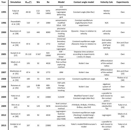
Year Simulation Θadv(o) We Re Model Contact angle model Velocity Calc Experiments
1995 Fukai et al.[43] 49-92 112-733 5476-14062 2-D axisymmetric Lagrangian deforming grid
Constant angle (Adv-Rec) Marker
velocity Own
1996 Pasandideh et al. [18] 110 27 2000
axisymmetric modified SOLA - VOF
Constant equilibrium angle/Dynamic from
experiment
N/A Own
2000 Bussmann et al. [58] 110 440 8000
piecewise linear volume
tracking method
Dynamic - linear in relation to velocity
cell center
velocity Own
2003 Francois et al. [59] 87.4 30 2772
immersed boundary method Eulerian-Lagrangian
Constant equilibrium angle /Dynamic linear in relation to
velocity
2nd marker point veloc (0.8*grid spacing)
Kim and Chun [22]
2005 Gunjal et al. [57] 35-110 3-567 924-10000
VOF - piecewise
linear
Stepwise time variation according to experiments
( every 15 steps)
N/A Own
2005 Sikalo et al. [50] 105 92 4018
VOF-based free-surface capturing method Kistler’s law differentiation of the wetted
radius
Own
2007 Mukherjee et al. [61] 87.4 30 2772 LBM Kistler’s law
differentiation of the wetted
radius
Kim and Chun [22]
2008 Caviezel et al. [55] 100 53 3245 Level Set Constant equilibrium angle N/A Rioboo et al. [30]
2008 Roisman et al. [41] 120 0.88-7.9 400-1200 VOF with Youngs interface tracking Kistler’s law algebraic system of equations Own
2009 Yokoi et al. [54] 107 32 22800 CLSVOF Modified Tanner's law/ Constant angle (Adv-Rec)
u parallel to wall closest to
the contact point x
own
2009 Shin et al. [47] 92 129 5878
level contour reconstruction
method
if θ>θadv, θ=θadv, if θ<θrec, θ=θrec, else θ=θ
shear strain rate(du/dn)
*Δx
Fukai et al. [43]
2012 Ganesan et al. [60] 105 92 4018
Lagrangian– Eulerian approach (ALE-FEM)
Constant equilibrium angle /Hocking’s model/Jiang’s
modle/Bracke’s model
Lagrangian Sikalo et al. [50]
2013 Griebel et al.
[56] 107 32 22800 Level Set
Yokoi’s model/Shikhmurzaev’s model
u parallel to wall closest to
the contact point x
[image:7.612.70.513.76.516.2]Yokoi et al. [54]
Table 1. Contact angle models and velocity calculation methods used in simulations from literature for water droplet impingement.
In Table 1, Fukai et al. [43] simulated impingement onto hydrophilic surfaces for a range of We numbers between 112 and 733. In other works, Ganesan et al. [60] simulated case #7 of Sikalo et al. (Table 2) which concerns the impingement of a water droplet onto a slightly hydrophobic wax surface (θadv =
105o) and afterwards presented their simulations for a droplet impact characterized by a very low
contact angle (θadv = 10o), without a comparison against experimental data. Gunjal et al. [57] simulated
surface. Vadillo et al. [21] showed that during the first milliseconds of a water droplet impingement onto two hydrophilic surfaces with equilibrium contact angles of 5o and 50o respectively, the dynamic contact
angle can reach values of approximately up to 80o-90o. The dynamic contact angle models presented in
Table 1 are representative of what has been documented in literature. For a more thorough, interesting and recent review of the available dynamic contact angle models, the readers can found information in the work by Saha and Mitra [70]. However, the question of how to simulate a priori a non-experimentally investigated case, for which contact angle data are not available, still remains to be answered.
Efforts towards the development of more complete models that can predict the dynamic change of contact angle during the droplet impact have also been reported. Roisman et al. [41] stressed out that the use of a dynamic contact angle model is very important in a CFD simulation, so that the temporal evolution of the phenomenon can be captured more accurately. Yokoi et al. [54] showed that in order to achieve a very good agreement between experimental data and simulation results, especially for the recoiling phase, the right use of a contact angle model is a necessity. In all the previously mentioned cases, the introduction of the contact angle between the droplet and the solid surface is achieved by specifying the contact angle (static or dynamic) as a boundary condition, i.e. as an input for the numerical simulation. This implementation has the basic drawback, that the dynamic contact angle is not a result of the simulated underlying physical mechanisms, and the induced fluid flow characteristics, but is dependent on the previously known values of contact angle temporal variation and the right calculation of the rim velocity.
In CFD simulations, especially using the VOF method, the extrapolation of the contact line velocity, when the interface of the droplet covers 2 or 3 cells, is not an easy process. Therefore, a new model needs to be developed that can dynamically alter the contact angle based on the induced fluid flow characteristics, rather than insert it as a boundary condition.
That is the basic aim of this study, i.e. to develop a new model that does not prescribe the contact angle (or its temporal evolution), but lets the net of forces acting on the free surface of the droplet (capillary, surface tension) and the 3-phase contact line to determine the liquid/gas interface interaction with the surface.
2.
Wettability
2.1
Dynamic contact angle models
Most dynamic contact angle models relate contact line velocity to the dynamic contact angle, which is inserted as a boundary condition. The dynamic contact angle models are briefly presented here below.
2.1.1 Quasi-dynamic contact angle mode (Advancing – Receding)
works of Pasandideh et al. [49] and Berberovic et al. [71]. The basic approach is simply represented by the two equations:
if u 0
dyn adv conline
( 2 )
if u 0
dyn rec conline
( 3 )
2.1.2 Kistler’s law
In the work of Kistler [72], the dynamic contact angle is given as a function of the contact line velocity through the Capillary number and the inverse of Hoffman’s function:
1
(
)
H dyn
f Ca f
H eq
( 4 )H x f x 0.706 0.99
arccos 1 2tanh 5.16
1 1.31 , (
1( ) H eq
x Ca f ) ( 5 )
.Ca liq conlineu
( 6 )
2.1.3 Shikhmurzaev’s model
Shikhmurzaev [73] gave a relation for the dynamic contact angle, as a function of several parameters, i.e.:
* *
1 2 0 1/2
*2 *
2 1
2 ( )
cos cos
(1 )
dyn eq
u a a u
a a u u
( 7 )
, *0 sin cos
sin cos
dyn dyn dyn
dyn dyn dyn
u
,a1 1 (1 a2)(coseqa4) ( 8 )
where a2=0.54 , a3=12.5 , a4=0.07 are phenomenological constants (values taken from [70]).
Basically, the dynamic contact angle models of Kistler and Shikhmurzaev try to deal with the difference observed in experiments between the dynamic contact angle (at microscopic length scale) and the apparent contact angle (at macroscopic length scale) within the inner region near the triple line point. A wide range of empirical correlations can be found in literature (a comprehensive review is presented in the work of Saha and Mitra [70]), that relate the contact line velocity with the dynamic contact angle in order to account for this inner region. This is also addressed in the works of Sikalo et al. [74] and Roisman et al. [41]. The differences in dimensionless spreading dynamics parameters (e.g. temporal evolution of spreading ratio, maximum spreading) which are observed between the simple quasi-dynamic model and these models may be related to that blurred distinction (Yokoi et al. [54]).
* 3
liq conlineu
u a
2.2
Wetting force model (WFM)
The idea behind the derivation of the Wetting Force Model comes from the work of Antonini et al. [75]. The authors investigated experimentally the adhesion force of a droplet sliding down an inclined surface and they derived a methodology for the prediction of this “adhesion” force. The “adhesion force” acts at the contact line, and is responsible for drop capillary adhesion to the surface. In their work [75], this adhesion force, for a contact line of arbitrary shape, is given by:
( 9 )
where L is the total length of the contact line, as visualized in Figure 1 (from [75]). For the validation of their methodology, the magnitude of the “adhesion” force was explicitly calculated, from the component of gravitational force (Figure 1a) acting on the droplet parallel to the solid surface, at the exact moment when it starts moving and for this specific angle of inclination.
[image:10.612.103.502.302.467.2]a b
Figure 1. Adhesion force. a) Droplet sliding down an incline. At the moment it starts moving, Fadhesionmgsina. b) Projection of the contact area of the droplet on the incline. Both Images taken from Antonini et al. [75]
Since the exact shape of the contact line and the complete contact angle distribution may be unknown, a simplified approach is typically used in many works , e.g. by Extrand and Kumagai [76], to estimate the capillary adhesion force. They refer to the adhesion force for solid/liquid/vapor systems, as being mathematically described by the following equation, both for static conditions, as well as dynamic conditions:
cos cos
adh
rec adv
f
K
r ( 10 )
where K is a fitting factor. In fact, the limit of this equation is the presence of the fitting factor K, which changes by changing the liquid-solid system.
Both the previously mentioned cases (Antonini et al. [75] and Extrand and Kumagai [76]) refer to static conditions (a droplet at rest onto a solid surface on the verge of starting to move), but a more complete model should be as well checked for its validation not only under stationary and/or quasi-steady conditions, but as well under dynamic ones. In this light, the scope of this study is to check the modelling
0cos cos L
adh
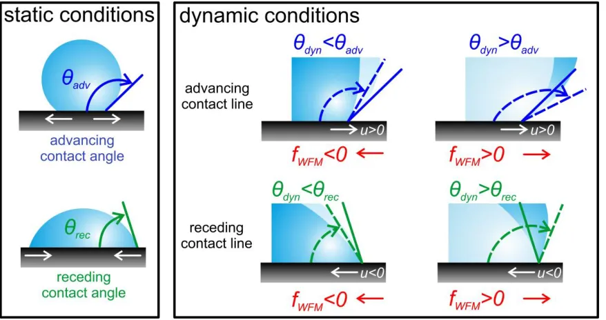
of an adhesion force model to the drop impact problem. The new model proposed considers for the effect that this additional (except from the standard interfacial tensions) contact line force will have - in relation to the “adhesion” force on the inclined surface or the one referred to in eq. 10 - on a spreading rate of a liquid droplet impacting onto both hydrophilic or hydrophobic surfaces. This additional term as implemented here describes the adhesion type force assumed to be parallel to the wall, as in Figure 2, and is expressed as:
dfWFM
(cos
eqcos
dyn)dl
(cos
eqcos
dyn) dr
( 11 ) [image:11.612.89.528.263.495.2]Where the equivalence dl rd
holds for a circular contact line, which is coherent with assumptions of axisymmetric flow for 2-D simulations. The direction of this stress term is presented in Figure 2 and is linked to the “adhesion” force reported before (eq. 10).Figure 2. Direction of the proposed adhesion term at the contact line for dynamic conditions: fWFM points to the left/right
until θeq is reached.
higher and its effect on droplet motion is stronger. Finally, since an axisymmetric case is considered, the force is proportional to the droplet radius (as one can verify from eq. 11).
The basic differentiation of the proposed model relative to previous works is the incorporation of this force into the Navier-Stokes momentum equation instead ofimposing a specific equilibrium or dynamic contact angle value as a boundary condition; from now on this approach will be referred as Wetting Force Model (WFM). In that way the microscopic change of the dynamic contact angle, as well as the macroscopic temporal evolution of the phenomenon, will change according to how this force aids or counteracts the droplet spreading onto the solid substrate. This stress term, therefore, would dynamically affect the formation of the dynamic contact angle in relation to its interaction with the standard surface tension force and viscous dissipation near the wall.
An additional advantage of this approach, when compared to the standard boundary condition (BC) approach, based on the work of Brackbill [69], is that by this methodology, one can really measure the temporal evolution of the dynamic angle the droplet forms, and compare this with available experimental data. This is shedding light on the complicated, not yet fully understood, underlying physical mechanisms controlling droplet impingement on any type of either flat or non-flat solid surfaces.
At this point, it should be mentioned that in their work, Sikalo et al. [50] in 2005 had already presented a study in which they impose as boundary condition the wetting force instead of a contact angle. In their simulations, however, this was only an alternative way to apply the Hoffmann’s law: the force applied at the contact line was calculated as function of the dynamic contact angle, which was derived from using the Hoffman’s law, or alternatively by the theoretical solutions based on creeping flow in the neighborhood of the contact line. In this study, the force does not depend on any law or empirical correlation, but relies on the value of the instantaneous contact angle.
3.
Mathematical modeling
3.1
Volume of Fluid Method
( 12 )
u t
( ) 0 ( 13 )
The solution of the aforementioned equations, in axisymmetric form, was performed in the commercial package of ANSYS FLUENT. The difference of VOF in comparison to other techniques is that a single momentum equation is solved for the two phases (gas – liquid), where the fluid properties are updated according to the volume fraction value of the cell:
(1 )
liq gas
( 14 )(1 )
liq gas
( 15 )Surface tension term fin the momentum equation is taken from the work of Brackbill et al. [69]:
( 16 )
where “κ” is the curvature of the free surface and is approximated as the divergence of unit surface normal, i.e.
n
ˆ ( 17 )n
ˆ ( 18 )
For a more accurate calculation of curvature, the unit surface normal vectors at the computational nodes are used. Pressure–velocity coupling is achieved by adopting a coupled approach [79] for which momentum and pressure-based continuity equations are solved together, while the Rhie-Chow pressure dissipation terms are included in the face mass fluxes [79]. Discretization of the momentum flux term is achieved by a second-order upwind scheme, while for the time discretization an first-order implicit approach is followed (explicit for volume fraction advection, eq. 13). The time-step of the calculations is varying for all simulations, so that the Courant number can be kept at around 0.25.
collisions [78, 85, 86] and impingement onto heated surfaces as reported in the works of researchers from the author’s group [52, 53, 65-67] .
3.2
Implementation of Dynamic contact angle models and Wetting Force
Model (WFM)
3.2.1 Dynamic contact angle models
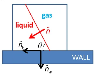
The dynamic contact angles, associated with the quasi-dynamic Adv-Rec, Kistler and Shikhmurzaev models, are implemented in the VOF model using a similar approach to the one presented in Brackbill et al. (eq. 53) [69] and Ubbink (eq. 2.22) [84]. The main idea lies on the use of a prescribed value of the contact angle θ at the wall as a boundary condition. Then based on this value, the normal to the
interface unit vector at the wall boundary cells nˆ is rotated, according to the following equation: ˆ ˆwcos ˆtsin
n n n
( 19 )
[image:14.612.223.384.316.443.2]so that the interface can form the prescribed angle θ, when in contact with the wall. Figure 3 is presented for better understanding of eq.19 concept and notation.
Figure 3. Unit vectors on the wall face, as well as unit free surface normal vector.
In particular, the rotation of this vector influences the interface curvature calculation (eq. 17) at the spreading droplet rim boundary cell, and in turn the surface tension force (eq. 16) applied at the cells. The calculation of the contact line velocity is based on the actual velocity calculated at each computational cell, in the close region of the rim (triple-phase contact region), from which the velocity component parallel to the wall ( ) is derived, according to eq. 20:
( 20 )
Although more accurate methods for contact line velocity have been presented in the literature, based on the time derivative of the radius of the wetted area, as in Sikalo et al. [50] and Roisman et al. [41] (ucontline=dxcontline/dt), the simple approximation used here can be easily extended to a three-dimensional
case. After the contact line velocity is found, the dot product of the velocity vector with the unit free surface normal provides the direction of contact line movement, i.e. if it the rim is advancing or recoiling.
If the resulting value is negative, this means that the rim is advancing ( always points inside the liquid phase), while if it is positive, the rim is recoiling.
In ANSYS FLUENT, a User Defined Function for the dynamic angle value is embedded. The function works as follows: a) it loops over all wall boundary cells, b) it calculates at each cell the contact line velocity (eq.20) along with the contact line direction (eq.21) and c) only at the cells where the volume fraction gradient is non-zero, a prescribed contact angle value is provided. In the background, this value changes the value of at the triple –phase contact region (max 3 cells), according to equation 19.
The choice of the non-zero gradient condition is chosen in accordance with Roisman et al. [41], who applied the contact angle boundary condition imposed on cells in the immediate vicinity of the transition region, characterized by the gradient of the VOF function. This is because the volume tracking algorithm provides a transition region, rather than the exact position of the contact line.
3.2.2 Wetting Force Model (WFM)
The proposed force term (eq. 11) is implemented into the Navier-Stokes momentum equation (eq. 12) as an extra source term, active only at the boundary cells in contact with the wall, in the vicinity of the interface. The theoretical correct way to implement this contact line force is to apply that only at one point, i.e. at the triple phase contact line. However, when the contact line is represented by more than one cell, especially in the case of droplet impacts on hydrophilic surfaces (low contact angle values), this stress term should also be applied in more than one cell, owed to the diffusion of the interface.
The “default” approach is to add this term at the cells in contact with the wall, where the volume fraction gradient is non-zero (as referred in Section 3.2.1). However, when this criterion was used for the application of the WFM, an unphysical velocity field was predicted at the contact line region, especially at the time instants when the droplet stopped advancing, right before the initiation of the recoiling phase.
To be more precise, at the time instant when the droplet stops advancing, the stress term which is applied at the contact line cells is such that the rim turns according to the receding contact angle. This results in the introduction of a force pointing towards the interface outward direction in numerous cells (max 3), which affects the local flow field and culminates in the unphysical breakup of small secondary droplets, Figure 4.
[image:15.612.73.496.546.661.2]t=9.2ms t=9.3ms t=9.4ms
Figure 4. Unphysical diffusion of volume fraction field, followed by the breakup of small secondary droplet observed when the Wetting Force is applied in a wide region around the contact line. Velocity vectors are plotted in the same manner for all pictures. The numerical tests have been performed for the conditions of Case 9.
ˆ
n
ˆ
n
α 0.9
0.5
As the contact angle hysteresis gets higher, this unphysical phenomenon becomes more intense. In order to avoid such unphysical behaviour, two alternative strategies can be implemented:
calculating the contact line velocity as the mass weighted average of all neighbouring cells to the reference cell, so that the contact line velocity can be closer to the liquid phase velocity;
considering, as an additional criterion for the application loci of the adhesion force, all the interface cells, i.e. the cells with the volume fraction ranging lower than a given small value for the gas phase and higher than a threshold value for the liquid phase.
The first test proved to be unsuccessful, while the second appeared valid for all cases examined (a large range of parameters), using the threshold values of 0.05 and 0.95 as the most representative for interface tracking.
The magnitude of which is implemented in the momentum equation is given by the following expression:
( 22 )
where
( 23 )
This stress term is divided by the cell volume in order to be consistent with the momentum equation (eq. 12). The equilibrium contact angle during the spreading phase is assumed to be equal to the advancing contact angle, , whereas during the recoil phase the equilibrium contact angle is equivalent to the
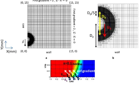
receding contact angle, . and are measured experimentally using the standard sessile drop method, i.e. while expanding and retracting a drop quasi-statically on a horizontal surface; their difference, , is the contact angle hysteresis. The method, based on which this dynamic contact angle is calculated, is crucial as it determines the magnitude of this force, and therefore its contribution to the net force. In this work, the dynamic contact angle was calculated from the slope of the normal to the free surface ( ) in the region near the contact line, as shown in Figure 5c.
At this point, the numerical procedure followed for the implementation of the wetting force is described: i. The contact line velocity (eq.20) and contact line direction (eq. 21) are found for all cells in
contact with the wall, where the volume fraction ranges in-between 0.05 and 0.95. For these cells, it is identified whether the contact line is advancing or recoiling.
ii. Subsequently, advancing or receding contact angles are inserted in eq. 22, in the place of θeq.
iii. The resulting source term is inserted in the momentum equation (eq. 12). For the cases examined in this paper, this additional stress term is inserted only in the radial velocity equation, since an axisymmetric approach is followed.
The particular case of a non-axisymmetric drop sticking to the substrate (with uconline = 0 and a
non-uniform distribution of contact angles on the entire contact line) should be treated in a different,
WFM
f
if u 0
if u 0
adv conline eq
rec conline
adv
rec
adv
rec
adv
recspecific way and it is not considered in the present paper. More specifically, in case of a sticking drop, e.g. a drop either under shear flow or on a tilted surface, the drop has a non-axisymmetric shape with a non-uniform distribution of contact angles. This causes the generation of a net adhesion force, which opposes to the external force (e.g. aerodynamic forces or gravity) and prevents drop motion. Predicting the onset of drop motion, when external forces overcome drop capillary adhesion, is not trivial, and can be complicated by the presence of surface local heterogeneities, as recently addressed by Varagnolo et al. [87] for the case of chemical heterogeneous surfaces with numerical simulations based on the lattice Boltzmann models. In the present paper, the main objective was not to evaluate the static adhesion force term, but to propose a model for the capillary adhesion force acting at the contact line in non-stationary and non-equilibrium impact conditions. To further extend the present work to study static and close-to-equilibrium conditions, such as the case of drops impacting on high hysteresis or tilted surfaces, one possibility could be to implement an adhesion force for the static case, such as:
, if uconline ( 24 )
where should be chosen near to the wetting velocity and generally r is the local curvature radius on the surface plane. This “static adhesion force” plays a role when the drop spreading stops and may have an influence both for the stick and slip behavior or for the time at the maximum spreading (Antonini et al. [38]). It is important to note that this force could also capture specific three-dimensional phenomena like the formation of lobes and the wavy rim on the surface.
3.3
Computational Domain, Boundary conditions, grid refinement
In Figure 5a, the basic 2-D axisymmetric domain, comprising of 60x60 identical quadrilateral cells is shown, where local grid refinement of the region around the droplet has been applied. This adaptive local grid refinement technique is selected in order to increase the numerical accuracy as much as possible, with the minimum computational cost, as will be discussed further in the following section. The initial wall-droplet distance, shown in Figure 5b, is selected to be one droplet diameter (D0) long so the
gas fluid flow around the droplet can develop in a physical way, just before droplet impact onto the surface. The initial droplet velocity and diameter are defined as Uo and Do respectively. Gravitational
acceleration is directed towards the positive values of x axis. It is very important to note that the initial domain for all computations, conducted in this paper, was the same, where the spatial coordinates (x- axial coordinate, y-radial coordinate) ranged between: X Y, 0 0.015m. Therefore, for the wide range of simulated cases presented in Table 2, the total length of the domain boundaries range between
0
(4 6.6D ) .
which was found to be far enough from the interface, so that the gradients of volume fraction are computed in the region with the denser grid cells. In that way, it is guaranteed that the computed surface tension term that will be inserted in the momentum equation will always have the highest level of accuracy.
Since such grid treatment is not given as a standard user option in ANSYS/FLUENT software, implementation of this technique was achieved through a User Defined Function (UDF). The method of refinement was based on the hanging node adaption, available in ANSYS FLUENT. In this work, four levels of refinement were used, achieving a minimum cell size of around Δxinitial/24 = 15.6μm. This
translates to approximately 72-120 cells along droplet radius for all the cases examined, which is in accordance to the current state-of-the art maximum grid resolutions applied in such cases. The application of this technique allows important computational time to be saved, as a uniform grid would require to be comprising of 921,000 cells uniformly distributed over the whole computational domain; for comparison, here only 24,672 cells are required for a typical droplet with initial diameter D0=2.75mm,
for the same grid resolution around the interface to be achieved.
a b
c
Figure 5. a) Initial Domain + Boundary conditions for all cases, b) Depiction of the local refinement technique, c) calculation of θdyn for the WFM.
3.4
Simulated cases
Nine cases are used for the validation of the proposed model; the corresponding conditions are summarized in Table 2 and concern the impingement of a water droplet onto both hydrophilic and hydrophobic surfaces. A wide range of We numbers ranging from as low as 0.2 up to 120 have been examined. Cases 1-4 refer to the impingement on hydrophobic surfaces, while Cases 5-9 concern
X(mm)
[image:18.612.79.524.316.589.2]hydrophilic surfaces. Case 6 (We=0.2) has been included in order to compare its results against those of Case 5, which also refers to a very low Weber number; it is known that for such very low Weber numbers, peculiar post-impingement liquid shapes are forming, as it will be further presented in a following section. The properties for liquid water and air that were used in the simulations are ρliq=998.2
kg/m3, μ
liq=1.003·10-3 kg/ms, ρgas=1.225 kg/m3, μgas=1.7894·10-5kg/ms.
Uo (m/s) Do (mm) θadv
(o)
θrec
(o) We Re
Dmax/D0 % dev
Ref
Cases
Run Exp Sim
Pasand Theory [18] WFM-Exp Pas-Exp 1.
LW-HCA-HH 0.48 2.50 120 65 8 1200 1.50 1.71 1.92 14.2 28.0 [41] 2.
MW-HCA-HH 1 2.28 107
(*90) 77 32 2280 2.29 2.42 2.59 5.7 12.9 [54] 3.
MW-HCA-LH 1.18 2.75 105 95 53 3245 2.62 2.85 2.95 8.8 12.4 [30] 4.
HW-HCA-LH 1.64 2.45 105 95 91 4018 3.1 3.30 3.29 6.5 6.2 [50] 5.
VLW-MCA-LH 0.22 2.40 70* 70 2 527 2.4 1.69 2.46 -29.6 2.4 [40] 6.
VLW-LCA-LH 0.08 2.30 31* 31 0.2 184 1.96 1.86 5.00 -5.1 155.0 [32] 7.
LW-MCA-LH 0.76 2.40 70* 70 19 1821 2.8 2.48 2.88 -11.4 2.7 [40] 8.
MW-LCA-LH 1.18 3.04 10 6 59 3587 3.31 3.62 4.22 9.4 27.6 [30] 9.
HW-MCA-HH 1.50 3.76 60
[image:19.612.75.541.164.424.2](*34) 22 117 5640 4.05 4.18 4.09 3.2 0.9 [43] Table 2. Test Cases used for the validation of the new model. Initial conditions are presented, together with results from the WFM, experiment and the theoretical correlations proposed by Pasandideh [18] (eq. 1). For the simplification of Cases, the following abbreviations are used: first the Weber number (W), then the advancing contact angle (CA), and finally the contact angle hysteresis (H), while the symbols VL , L , M , H represent the words very low, low, moderate and high. (* equilibrium angles (Cases2,9). When only the equilibrium angle is given, the advancing/receding angles take this value, as in Cases5-7.)
4
Results and discussion
In this section the results obtained are presented. Initially, a brief grid dependency study will be presented together with results for validating the global behavior of the model. Then, detailed predictions for the temporal evolution of the relevant phenomena are presented: Initial predictions for the evolution of the dynamic contact angle are given followed by the corresponding ones for hydrophobic and hydrophilic cases.
4.1
Grid size verification
For a thorough validation of the model, and due to the fact that in the present simulations the dynamic contact angle is calculated, the effect of grid size on the numerical results should be investigated, so as to prove that the magnitude of the force exerted, in relation to the surface tension force, is not mesh-dependent. For that reason, Cases 1 (LW-HCA-HH) and 7 (LW-MCA-LH) were run using six levels of local refinement, achieving a minimum cell size of around Δx/26 = 3.9μm. The results for these cases were
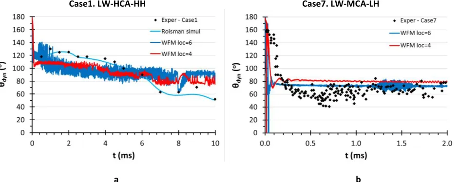
the default choice for this study. Figure 6 presents the temporal evolution of the calculated dynamic contact angle, measured from the volume fraction 0.5 iso-line passing from the reference cell (one cell in contact with the wall), after the application of the Wetting Force Model using 4 (default) and 6 levels of local refinement respectively, in comparison to the available experimental values. Moreover, for Case1(LW-HCA-HH)the experimental data of Roisman et al. [41] are well fitted. It is clear that the effect of grid size is minimal both for hydrophobic (Figure 6a) and hydrophilic (Figure 6b) surfaces, even if in the latter case, the results for the dynamic contact angle are slightly improved by the application of 6 levels of local refinement. The “noise” observed in Figure 6a can be attributed to the very small cell size, in relation to the sign change of the applied wetting force. More precisely, as the reference cell size (where contact angle is measured) gets smaller, the interface is more prone to direction changes owed to a) velocity field fluctuations and b) the application of an updated stress magnitude at each time instant. Additionally, one should not forget that at each time instant the curvature of the interface changes, which in turn affects the induced velocity field and therefore the formed contact angle. This in turn affects the exerted on that cell stress magnitude. Moreover, one could imagine that this oscillating behavior, presented in Fig.4a, may resemble the pinning of droplet during its spreading between two values as stated by [89], but this should be further investigated.
The same behavior is observed for Case7 (LW-MCA-LH), at the time when the dynamic contact angle reaches the set equilibrium value (θ=70o, Table 2). On the whole, the numerical results are not
considered to be highly dependent on the level of local grid refinement and given the fact that 6 levels of local refinement is computationally too expensive, the numerous cases presented in this paper are run using 4 levels of local refinement.
Case1. LW-HCA-HH Case7. LW-MCA-LH
[image:20.612.76.547.419.606.2]a b
Figure 6. Effect of grid size for Cases 1. LW-HCA-HH and 7. LW-MCA-LH of Table 2 a) θdyn as a result of the WFM simulation
using 4 and 6 levels of local refinement in comparison with the experimental values and simulation results of Roisman et al. [41]. b) θdyn as a result of the WFM simulation using 4 and 6 levels of local refinement in comparison with the experimental
values of Roux et al. [40]. The symbol “rm” in the graphs stands for remeshing.
4.2
Global performance of the model
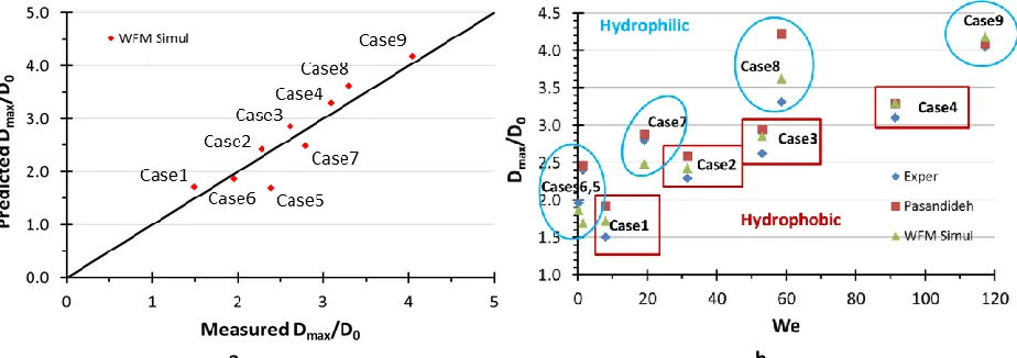
with the exception of Case5 (VLW-MCA-LH). Similarly, Figure 7b presents the maximum dimensionless spreading as a function of Weber number; here 3 sets of data have been included: a) WFM predictions, b) experiments and c) the estimates of the Pasandideh’s correlation (eq. 1). The results obtained by application of the Pasandideh’s equation overestimate the experimental droplet maximum spreading1,
while the WFM model predicts accurately the impingement onto dry hydrophobic surfaces, even if it is less accurate for the hydrophilic ones, particularly for moderate Weber numbers. Concerning the hydrophobic surfaces, results of the WFM slightly overestimate (approx. 10%) the experimental findings. On the other hand, for hydrophilic surfaces, not a monotonic overestimation or underestimation of the model predictions against experimental data is tracked.
[image:21.612.76.538.223.386.2]a b
Figure 7. Summary of simulation results with the use of WFM model. a) Droplet maximum spreading plotted against the experimental values, b) Maximum spreading plotted against experimental values and results of eq (1).
Being able to predict the droplet maximum spreading for a variety of contact angles and Weber numbers, it can be claimed that the WFM can be trusted; moreover, a simple grid dependency study showed that the results are not mesh affected. After that, a more detailed comparison of the model predictions will follow in the forthcoming sections.
4.3
Dynamic contact angle evolution
The results of the dynamic contact angle predictions for both hydrophobic and hydrophilic surfaces presented in Figure 6 serve as a sign of validity for the new model (WFM), which as noted above can shed light in the temporal evolution of the phenomenon by not prescribing a contact angle value, but on the other hand predicting it. For hydrophobic surfaces, as stated in the Introduction section, only the study of Roisman et al. [41] exhibits dynamic contact angle measurements and thus can be used for validation; in Figure 6a the predictions of the WFM and experimental data are shown for Case1 (LW-HCA-HH), accompanied by the corresponding numerical results presented in the work of Roisman et al. [41], who used the Kistler’s dynamic contact angle model (eq. 6). The dynamic contact angle predicted by the WFM during the advancing phase is lower than the one measured during the experiments, which is a reason for the over-prediction of maximum spreading (Case1 in Figure 7).
1
It should be mentioned that Pasandideh equation is not applicable for very low Weber numbers, because the assumption of a
During the initial stage of impingement, as soon as the liquid droplet comes in contact with the surface, θdyn is approximately 180o. Subsequently, the contact angle reduces rapidly to approximately 110o,
which is lower than the equilibrium angle accounted for in eq. 22 (i.e. the advancing one, 120o) and
slowly reduces during the rest of the advancing phase. θdyn then drops suddenly to 80o at approximately
6.5ms, which can be set as the initiation of the receding phase; this value is higher than the equilibrium value of 65o set in Eq. 22. This shows that the application of the wetting force has smaller effect than
expected. Contact line velocity exhibits similar behavior (presented in Figure 8). At first, a spike is observed when the droplet hits the surface, followed by an almost exponential reduction of its magnitude with time. The time interval between 5 and 6.5ms is considered to be the “hysteresis” time, i.e. the time needed for the contact angle to decrease from values ~θadv to ~θrec. During this stage, the
contact line velocity fluctuates around zero. At later stages, t > 6.5ms, contact line velocity exhibits negative values, i.e. the droplet is recoiing, with substantially smaller magnitude than during the advancing phase.
Case1. LW-HCA-HH
Figure 8. Contact line velocity throughout the impingement for Case1. LW-HCA-HH.
In Figure 6b, the dynamic contact angle for Case7 (LW-MCA-LH) is compared against the experimental values of Roux et al. [40]. During the initial stage of impingement, the contact angle starts with a value again of 180° and drops again quite fast down to 80o. This trend is also observed in the experimental
data; however, the duration of this period is underestimated by the simulation. Afterwards, a constant angle of around 80° is predicted by the model, while the experimental values lie between 50° and 80°. This harmony between simulation and experiment is also confirmed by the agreement in droplet shapes depicted in Figure 17, which will be presented in the following sections.
4.4
Wetting Force Magnitude
much more intense, which however does not exhibit any significant changes in the macroscopic simulation of the phenomenon of liquid droplet impact on a solid flat surface.
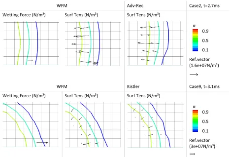
WFM Adv-Rec Case2, t=2.7ms
Wetting Force (N/m3) Surf Tens (N/m3) Surf Tens (N/m3)
Ref.vector (1.6e+07N/m3)
WFM Kistler Case9, t=3.1ms
Wetting Force (N/m3) Surf Tens (N/m3) Surf Tens (N/m3)
[image:23.612.67.534.111.429.2]Ref.vector (3e+07N/m3)
Figure 9 Magnitude of the Wetting Force, as well as surface tension force predicted by the WFM in a random time instant compared to the surface tension force predicted by Kistler’s model. Force vectors are plotted in the same manner for both Cases (using the value of 3e-08 cm/magnitude).
Additionally, if the WFM was simply turned off, the resulting contact angle at the wall boundary would be approximately 90o, since the applied BC would have been that of a zero Neumann boundary
condition ( ).
4.5
Spreading on hydrophobic surfaces
In Figure 10, the temporal evolution of the impingement of a water droplet onto solid hydrophobic surfaces is depicted for the Cases 1-4 of Table 2. More specifically, results from the application of WFM are compared against the corresponding experimental data; in addition, the predictions obtained using the dynamic contact angle models of Kistler and Shikhmurzaev, as well as those obtained by assuming fixed advancing-receding angles are also indicated. Furthermore, in the same figures, results reported in the literature by other researchers for the same cases and referenced in Table 2 have been also included. Exception to this is Case3 (MW-HCA-LH), since previous simulation results cannot be found in literature to the best of the author’s knowledge; it is noted that the results of Caviezel et al. [55], that also refer to this case, present only comparison against corresponding photographs during the impingement process
x y
ˆ
ˆ
n =0, n =0
α 0.9
0.5
0.1
α 0.9
0.5
but the temporal evolution of the spreading radius has not been provided in the corresponding reference.
Case1. LW-HCA-HH. We = 8 Case2. MW-HCA-HH. We = 32
[image:24.612.74.549.115.448.2]Case3. MW-HCA-LH. We = 53 Case4. HW-HCA-LH. We = 91
Figure 10. Comparison of WFM results against experiments and respective simulations for the hydrophobic surfaces of Cases1-4 listed in Table 2(where references can be found); corresponding predictions from other dynamic contact angle models found in literature are also indicated.
In general, the Wetting Force Model overestimates slightly the maximum droplet spreading. Given that the proposed model calculates the contact angle rather than using it as a boundary condition, a good agreement between the results derived from the WFM and the experiments can be claimed. It should be noted that contact angle predictions, as provided by the Shikhmurzaev’s and Kistler’s models as function of the contact line velocity assuming an arbitrary θeq= 90o can give up to 20% difference. This suggests
that significant differences when predicting the contact angle can be expected with all the previous models.
experiment suggests (for example at t=20.54ms, in simulation results, the break-up of the satellite droplet has occurred, while in the experiment this phenomenon occurs later). Similar results are presented by Caviezel et al. [55], indicating a very good agreement between the results of the two codes. In Figure 8, the isosurface =0.5 is depicted, where the interior of the droplet is cut in order to present both the dynamic grid refinement technique and velocity vectors throughout the impingement process. Moreover, the pressure of the liquid phase is shown for the boundary wall cells. For the non-dimensionalisation of these parameters, velocity magnitude is divided by the initial impact velocity, while pressure is divided by the initial kinetic energy of the droplet, thus defining the pressure coefficient as:
2 2
0
1 1
2 2
momentum p
liq
P P P C
U U
( 25 )
In this equation, Poo and Uoo are the velocity and pressure on the far field. The pressure difference is
given by the value of pressure evaluated in the momentum equation.
TIME (ms)
WFM Exper (Rioboo et al.) [30]
t=0
t=1.31
t=3.14
t=6.02
C
0 10
2.5 5 7.5 U/U0
0.05 5
0.15 0.5 1.5
C
0 1.1 5
t=10.26
t=14.02
[image:26.612.73.496.69.483.2]t=20.54
Figure 11. Comparison with experiment for Case 3. MW-HCA-LH (Rioboo et al. [30]). Pictures taken from reference. Results are represented in 3 dimensions, after the revolving of symmetry axis. Cp contour and velocity vectors colored by velocity
magnitude are plotted. Cp values below 0.01 are cutoff. The first Cp contour legend applies to the first two pictures, while
the second one applies to all the following. Velocity contour is the same for all pictures.
At the initial stage of impingement, t=0–1.31ms, pressure can reach up to 9.7 times of droplet initial kinetic energy, which can be explained by pressure rise due to formation of a dimple upon drop impact [90]. During the rest of the spreading phase and the start of the recoiling phase (t=3.14-6.02ms), Cp is
In Figure 12, the comparison between pictures taken from the work of Sikalo et al. [50] (Case4 HW-HCA-LH) are compared against the results of the WFM simulation. Again, very good qualitative agreement is observed between simulation and experiment. In this figure, the pressure contours, as well as the induced flow field during the process are presented.
t = 0.05 ms t = 0.86 ms
t = 1.25 ms t = 1.95 ms
t = 3.86 ms t = 4.67 ms
t = 5.7 ms
t = 7.8 ms
Figure 12. Comparison with experiment for Case4. HW-HCA-LH (Sikalo et al. [50]). Pictures taken from reference. Cp contour and velocity vectors colored by velocity magnitude are plotted. Cp values below 0.01 are cutoff. The first contour legends
apply to the first picture, while the second one applies to all the other.
X/R0 X/R0
X/R0 X/R0
X/R0 X/R0
X/R0 X/R0
Cp
1.6 11.4
4.9 8.1
Y/
R0
Y/
R0
Y/
R0
Y/
R0
Cp
0.0 1
0.9
0.3 0.6
U/U0
0.1 1.5
0.5 1.1 U/U0
0.3 5
Typical impingement behavior is again observed in these pictures, where during the initial stage of the process, velocity magnitude reaches up to 4 times the initial impact velocity. Moreover, the vortex on the top of droplet rim is again visible, while it changes direction between 3.86ms and 4.67ms (receding phase). At the moment when the droplet hits the surface, Cp can reach up to 10 times the initial kinetic
energy of the droplet, while for the rest of the process the maximum one is only 0.85 of the initial kinetic energy Finally, in the last picture, at t=7.8ms, the ejection of a small droplet on the symmetry axis is predicted, which comes from the quick break-up of the droplet in the symmetry axis, just as the liquid mass was retracting.
In Figure 13, the non-dimensional spreading radius is plotted against time, for all 4 cases concerning the impingement of a water droplet onto hydrophobic surfaces. It is clear that at the first stage of impingement (τ=t Uo/Do < 0.2) the four lines coincide in one, depicting the uniform character of the
[image:28.612.169.401.281.429.2]impingement process, which has been also reported by Rioboo et al. [30].
Figure 13. Non-dimensional spread factor from WFM simulation plotted against non-dimensional time for hydrophobic surfaces. θadv= 105o-120o. We=8-91, x-axis, logarithmic scale.
4.6
Spreading on Hydrophilic surfaces
Case5. VLW-MCA-LH. We = 2 Case7. LW-MCA-LH. We = 19
[image:29.612.74.544.74.410.2]Case8. MW-LCA-LH. We = 59 Case9. HW-MCA-HH. We = 117
Figure 14. Comparison of WFM results against experiments and respective simulations for the hydrophilic surfaces of Cases5,7-9 listed in Table 2 (where references can be found); corresponding predictions from other dynamic contact angle models found in literature are also indicated.
The first two experimental cases presented in Figure 14 are taken from the work of Roux et al. [40] and concern the impingement of a water droplet onto a hydrophilic surface at low Weber numbers (We=2 and 19). In their work, Roux et al. [40] give experimental measurements for the time evolution of droplet radius only for the first 4ms of the impingement, while they present the droplet maximum radius in one Figure relating that to the Reynolds number. Therefore, the comparison between model and experiments for these cases is limited to this specific time interval (initial 4ms), while the respective comparison with the value of maximum spreading is given in Table 2 and presented in Figure 7.
For Case8 (MW-LCA-LH), a significant over-prediction of droplet spreading is predicted by the simulation, as it is shown in Figure 14. This Case is taken from the work of Rioboo et al. [30] where it is reported that the advancing contact angle takes the value of 10 degrees (Table 2). Using this value, none of the dynamic contact angle models was able to reach a non-dimensional maximum diameter of 3.31 as measured in the experiments. The Wetting Force Model, on the other hand, predicts a non-dimensional spreading substantially lower than the other models and significantly closer to the experiments. Additionally, the recoiling of the drop is predicted, unlike to what the experiment suggests and this is the reason that the results for only the first 15ms are presented.
Finally, for Case9 (MW-LCA-LH), all models seem to behave better than previously, and the maximum spread is well captured. Shikhmurzaev’s dynamic contact angle model gives the best results among all the standard used contact angle models. For once more, the Wetting Force Model, seems to behave slightly better during the advancing phase, but predicts a quicker recoiling phase. In Figure 15 the prediction of “hysteresis” time for Case 9 is depicted for the WFM model in comparison to the advancing-receding model. Firstly, it is obvious that the hysteresis time lasts much longer for the Advancing-Receding model. This is shown by the “turning” of the rim at time instant t=13.66ms for the Advancing-Receding model, in conjunction with the slight “turn” in 9.93ms for the Wetting Force Model.
Constant values for Advancing/Receding CA WFM
t=8.09 ms t=7.76 ms
t=13.66 ms t=9.93 ms
t=31.68 ms t=15.62 ms
Figure 15. Prediction of “hysteresis” time for WFM in comparison to Advancing-receding model. Velocity vectors colored by velocity magnitude are plotted. Higher receding angle which results in quicker recoiling phase is predicted by the WFM.
Secondly, it is evident that the receding contact angle that is formed is not the same for the two models. The Wetting Force Model predicts a higher receding contact angle, which is the main reason for the quicker recoiling phase, as observed in Figure 14. Finally, on the third picture (15.62ms for the WFM) it is
X/R0
3 3.5 4 4.5 0.4 0.3 0.2 0.1 0 Y/ R 0 X/R0
3 3.5 4 4.5 0.4 0.3 0.2 0.1 0 Y/ R0 X/R0
3 3.5 4 4.5 0.4 0.3 0.2 0.1 0 Y/ R0 X/R0
3 3.5 4 4.5 0.4 0.3 0.2 0.1 0 Y/ R0 X/R0
3 3.5 4 4.5 0.4 0.3 0.2 0.1 0 Y/ R 0 X/R0
obvious that the highest angle that is formed using the WFM results in the prediction of a different flow field (vortex over the rim), which additionally has higher receding velocity values. Thus, a quicker receding phase is observed. The simulation stopped at 30ms because droplet break-up in the symmetry axis was observed, and the present axisymmetric application of the Wetting Force Model cannot be considered as valid after that time instant. Finally, the direction turn of the vortex which lies on top of droplet rim is obvious in the transition from advancing to receding phase.
In Figure 16 and Figure 17 the shape of the drop at characteristic times during the impingement of Cases 5 (VLW-MCA-LH) and 7 (LW-MCA-LH) is presented. In Figure 16 the phenomenon is captured qualitatively.
Case5. VLW-MCA-LH - Exper (Roux et al.) We=2
texp = 0.089, 1.157, 3.314, 4.272, 8.455, 10.146 ms
[image:31.612.77.516.223.621.2]tsim = 0.089, 0.53, 1.5, 3.4, 5.49, 6.21 ms
Figure 16. Comparison with experiment for Case5. VLW-MCA-LH. Cp contour and velocity vectors colored by velocity
magnitude are plotted. Cp values below 0.01 are cutoff. The first contour legends apply to the first 3 pictures, while the
second one applies to all the other.
However, as it was also observed in Figure 14, droplet initial spreading is overestimated, meaning that the phenomenon is predicted to be much quicker that in real time. This is evident in Figure 16, where the simulation time is much smaller than the real time. Moreover, in the first 4 experimental pictures,
X/R0 X/R0 X/R0
X/R0 X/R0 X/R0
Cp
5 12
8.5
U/U0
0.6 7
2.2
Cp
3 24
13.5
U/U0
0.1 6


![Table 2. Test Cases used for the validation of the new model. Initial conditions are presented, together with results from the WFM, experiment and the theoretical correlations proposed by Pasandideh [18] (eq](https://thumb-us.123doks.com/thumbv2/123dok_us/1517127.104321/19.612.75.541.164.424/validation-conditions-presented-experiment-theoretical-correlations-proposed-pasandideh.webp)