HAR Modeling for Realized Volatility Forecasting

City, University of London Institutional Repository

Citation

:

Corsi, F., Audrino, F. and Reno, R. (2012). HAR Modeling for Realized Volatility

Forecasting. In: Handbook of Volatility Models and Their Applications. (pp. 363-382). New

Jersey, USA: John Wiley & Sons, Inc. ISBN 9780470872512

This is the accepted version of the paper.

This version of the publication may differ from the final published

version.

Permanent repository link:

http://openaccess.city.ac.uk/4438/

Link to published version

:

http://dx.doi.org/10.1002/9781118272039.ch15

Copyright and reuse:

City Research Online aims to make research

outputs of City, University of London available to a wider audience.

Copyright and Moral Rights remain with the author(s) and/or copyright

holders. URLs from City Research Online may be freely distributed and

linked to.

City Research Online:

http://openaccess.city.ac.uk/

[email protected]

CHAPTER 1

HAR MODELING FOR REALIZED

VOLATILITY FORECASTING

Fulvio Corsi (University of St. Gallen), Francesco Audrino (University of St. Gallen),

1

Roberto Ren `o (University of Siena)

2

3

1.1 INTRODUCTION

4

The importance of financial market volatility has generated a very large literature

5

in which volatility dynamics has been modelled in order to take into account its

6

most salient features: clustering, slowly decaying auto-correlation, and non-linear

7

responses to previous market information of a different type.

8

In the literature, these phenomena have typically given rise to models in which

9

volatility is generated by a long memory process, characterized by fractional

inte-10

gration and an hyperbolic decay of the autocorrelation function. However, in this

11

chapter we follow an alternative direction which generates very similar stylized facts

12

for volatility series using the superposition of short memory frequencies. This

frame-13

work turns out to be easier to handle, with a straightforward economic interpretation

14

and an excellent fit to the data.

15

Volatility Models and Their Applications. By Bauwens, Hafner, Laurent

Copyright c2011 John Wiley & Sons, Inc.

Originally, this framework was inspired by the work of [66] and [41]. We view

1

volatility persistence as the result of the aggregation of the heterogeneous components

2

present in the financial market (the so called Heterogeneous Market Hypothesis).

Het-3

erogeneity among participants in the financial market may be of a different nature:

4

differences in the endowments, institutional constraints, risk profiles, information,

5

geographical locations, and so on. The proposed model concentrates on the

het-6

erogeneity that originates from (or materializes in) the difference in time horizons.

7

Typically, a financial market is composed of participants having a large spectrum

8

of trading frequencies. At one end of the spectrum are dealers, market makers,

9

and intraday speculators with an intraday trading horizon. At the other end, there

10

are institutional investors, such as insurance companies and pension funds trading

11

much less frequently and possibly for larger amounts. The key idea is that agents

12

with different time horizons perceive, react to, and cause different types of volatility

13

components.

14

In addition, it has been recently observed that volatility over longer time intervals

15

has stronger influence on volatility over shorter time intervals than conversely.1This

16

can be economically explained by noticing that for short-term traders the level of

17

long-term volatility matters because it determines the expected future size of trends

18

and risk. The overall pattern that emerges can be statistically described by a cascade of

19

heterogeneous volatility components (generated by the action of market participants

20

of different natures) from low frequencies to high frequencies.

21

This idea has been pursued in [34], who proposed an additive cascade model

22

of realized volatility aggregated at different time horizons. This cascade of

het-23

erogeneous volatility components leads to a simple AR-type model in the realized

24

volatility that considers volatilities realized over different time horizons and is thus

25

called Heterogeneous Auto-Regressive (HAR). In spite of its simplicity and the fact

26

that it does not formally belong to the class of long-memory models, the HAR model

27

for realized volatility is able to reproduce the volatility persistence revealed by the

28

empirical analysis on financial markets. The combination of ease of implementation

29

with a very accurate fit of financial volatility time series has made the HAR models

30

very popular in the financial econometrics community.

31

In this chapter we survey the HAR model for realized volatility forecasting and

32

its extensions. After reviewing some stylized facts of realized volatility we present

33

the derivation and possible interpretations of the heterogeneous structure of the HAR

34

model. We then discuss different extensions of the univariate HAR model aiming at

35

modeling the forecasting power of jumps, leverage effect and structural breaks.

36

In particular, we provide evidence for the contention that jumps have

signifi-37

cant impact on future realized volatility and that the impact of negative returns (the

38

so-called leverage effect) is highly persistent and also presents a HAR structure,

39

confirming the view of the existence of an heterogeneous structure in the financial

40

market. Moreover, we also provide empirical evidence of the existence of other

non-41

linear effects of past market information on volatility on the top of the leverage effect

42

STYLIZED FACTS 3

by introducing a flexible HAR-type model able to explicitly take into account

struc-1

tural breaks and regime-switches. Finally, we provide a brief review of multivariate

2

models for realized variance-covariance matrix dynamics.

3

1.2 STYLIZED FACTS ON REALIZED VOLATILITY

4

Summarized from the vast literature on the empirical analysis of financial markets,

5

the main characteristics of financial markets volatility are:

6

1. Long range dependence: (hourly, daily, weekly and monthly) realized volatility

7

displays significant autocorrelations even at very long lags. This property is

8

often ascribed to a long memory data generating process. In this chapter, we

9

take another approach by using a superposition of autoregressive processes

10

with different time scales.

11

2. Leverage effect: it is empirically observed that returns are negatively

corre-12

lated with (realized) volatility. In particular, volatility bursts are more likely

13

associated with negative past returns.

14

3. Jumps: financial prices are subject to abrupt variations. Jumps are not very

15

frequent and practically unpredictable, but they have a strong positive impact

16

on future volatility.

17

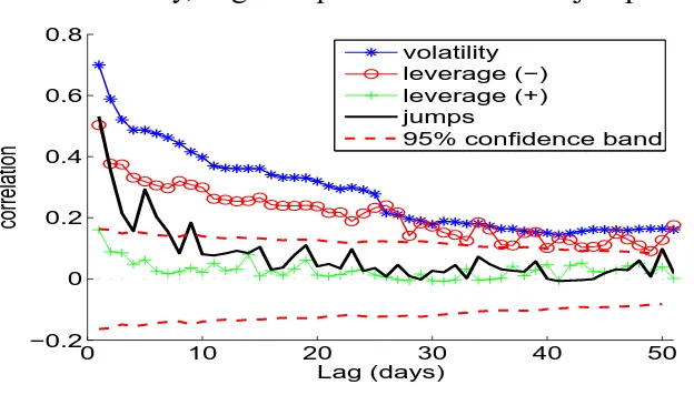
To illustrate these stylized facts of realized volatility (RVt), let us now consider

18

historical data on the S&P 500 stock index over the period 1982-2009. Figure 1.1 plots

19

Corr(RVt, Zt−h), i.e. the correlation betweenRVtandZt−h, forh= 1, . . . ,50.Zt

20

corresponds either toRVt, negative daily returns (r−t =min(rt,0), wherertis the

21

return on dayt), positive returns (r+t =max(rt,0)) or jumps (Jt). More details on the

22

data and the estimation ofRVtandJtare given in Section 1.3. Corr(RVt, RVt−h)

23

is the AutoCorrelation Function (ACF) of RVt. Figure 1.1 clearly suggests the

24

presence of long-memory in the realized volatility. This figure also suggests that

25

while past positive daily returns (r_t+_−h) are not significantly correlated withRVt, past

26

negative returns (r_t−_−h) have a significant impact on futures volatilities, and negative

27

shocks take a long time to die out (which might also be viewed as long-memory).

28

Interestingly, jumps seem also to have a positive impact on future values ofRVt,

29

although their effect decays at a faster rate thanRVtandr−_t−h. This motivates the

30

analysis in the following sections.

31

1.3 HETEROGENEITY AND VOLATILITY PERSISTENCE

32

The appearance of long range dependence might be due to a genuine long-memory

33

data generating process or, alternatively, it can be explained as a combination of

34

different short memory processes (as discussed further below). Although a true long

35

memory process requires the aggregation of an infinite number of short memory

36

processes (as shown by [52]), an approximated long memory process (practically

Correlation between realized volatility and past realized

volatility, negative/positive returns and jumps.

0 10 20 30 40 50

−0.2 0 0.2 0.4 0.6 0.8

Lag (days)

correlation

volatility leverage (−) leverage (+) jumps

95% confidence band

Figure 1.1 Corr(RVt, Zt−h) (h = 1, . . . ,50) for the S&P 500 series for the period January 1990 to February 2009. Ztcorresponds either toRVt, negative daily returns (r−t =

min(rt,0), wherertis the return on dayt), positive returns (r+t =max(rt,0)) or jumps (Jt). The displayed95%confidence bands (dashed lines) are computed with the generalized Bartlett’s formula of [46].

indistinguishable from a true one) can be obtained by aggregating only few

hetero-1

geneous time scales ([58]).

2

The need for multiple components in the volatility process has been advocated

3

by (among others) [66], [43], [21], [14], and [26] and has been reconsidered by

4

making use of the concept of an additive cascade of realized volatility aggregated

5

over different time horizons in [34]. In what follows, we briefly review this latter

6

approach.

7

We assume that the state variableX (typically the log price) is driven by the stochastic process:

dXt=µtdt+σtdWt+ctdNt, (1.1)

whereµtis predictable,σtis c´adl´ag andNtis a doubly stochastic Poisson process2 whose intensity is an adapted stochastic processλt, the random times of the corre-sponding jumps are(τj)j=1,...,NT andcjare iid adapted random variables measuring

the size of the jump at timeτj. In practice, e.g. for risk management purposes, we

HETEROGENEITY AND VOLATILITY PERSISTENCE 5

are interested in forecasting the quadratic variation defined as:

e

σ2t = Z t+1

t

σs2ds+ X

t≤τj≤t+1

c2τj,

where the time unit is one day.

1

This quantity is not directly observable and therefore has to be estimated. Let us denote byVˆta consistent estimator ofσe2t, that is:

log_eσt2= log ˆVt+ωt,

whereωtis iid noise.3 In the ideal case of no microstructure noise,RVtis the most

2

natural choice forVˆt. In the presence of microstructure noise, other estimators are

3

preferable such as the two-scale estimator proposed by [74], the realized kernels

4

method of [13], the pre-average approach of [55], or the multi-scales Discrete Sine

5

Transform estimator (DST) of [40]. In our empirical analysis in Section 1.6, we use

6

theDSTestimator.

7

Consider the aggregated values oflogVbt, defined as:

logVb(tn)=

1

n

n X

j=1

logVbt−j+1 (1.2)

and assume two different time scales, of lengthn1andn2, withn1> n2(e.g. weekly

and daily). For the largest time scale, assume thatσ_e2

t, once aggregated as in (1.2), is determined by:

logσ_e2,(n1)

t+n1 =c

(n1)_+β(n1)_logVb(n1)

t +ε

(n1)

t+n1 (1.3)

whereε(n1)

t is an iid random variable with mean zero and unit variance which is

8

independent on the estimation errorωt, andc(n1)andβ(n1)are unknown parameters.

9

This can be explained by assuming that the level of short-term volatility does not affect the trading strategies of long-term traders.4 On the other hand, for short-term traders the level of long-term volatility matters because it determines the expected future size of trends and risk. Hence, the shorter time scale(n2)is assumed to be

influenced by the expected future value of the largest time scale(n1), so that:

logσe2,(n2)

t+n2 =c

(n2)_+β(n2)_logVb(n2)

t +δ( n2)_E

t h

logeσ2,(n1)

t+n1

i

+ε(n2)

t+n2, (1.4)

whereε(n2)

t is an iid random variable with mean zero and unit variance, independent onε(n1)

t andωtandδ(n2)is a constant. The economic interpretation of this mech-anism is that each volatility component corresponds to a market component whose

3_{The model can also be specified in terms ofbV} tand for

q b

Vt, as in [34] [3] and [38]. However, the log specification has the double advantage of avoiding imposing positivity constraints and making the distribution closer to normality, see e.g. [51].

expectation on next period volatility is formed looking at, beyond the current realized volatility value, the forecast on the longer time horizon. The basic idea is that agents with different time horizons perceive, react to, and cause different types of volatility components. By substitution, this gives:

logVb(tn+2n)2 =c+β

(n2)_logVb(n2)

t +β(n1)logVb

(n1)

t +εt; (1.5)

whereεtis iid noise depending onε

(n1)

t , ε

(n2)

t , ωt. The model (1.5) can be easily

1

extended todhorizons of lengthn1> n2> . . . > nd. Typically, three components

2

are used with lengthn1= 22(monthly),n2= 5(weekly),n3= 1(daily).

3

The HAR model is then a parsimonious AR model reparameterized by imposing

4

different sets of restrictions (one for each volatility component) on the autoregressive

5

coefficients of the AR model. Each set of restrictions takes the form of equality

6

constraints among the autoregressive coefficients constituting a given time horizon,

7

so that once combined they lead to a step function for the autoregressive weights.

8

In this sense, the HAR can be related to the MIDAS regression of [47], [48], and

9

[45], although the standard MIDAS with the estimated Beta function lag polynomial

10

cannot reproduce the HAR step function weights.

11

In practice, the HAR model provides a simple and flexible method to fit the

12

partial autocorrelation function of the empirical data with a step function which has

13

predefined tread depth and estimated (by simple OLS) rise height. More generally,

14

however, nothing prevents the use of different types of kernel in the aggregation of

15

b

Vtinstead of the rectangular one used in the simple moving average; in this case we

16

would no longer have a step function for the coefficients but a more general function

17

given by a mixture of kernels (e.g. mixture of exponentials for exponentially weighted

18

moving averages) which can still be easily estimated by simple OLS.

19

Even if the HAR model does not formally belong to the class of long memory

20

processes, it fits the persistence properties of financial data as well as (and potentially

21

better than) true long memory models, such as the fractionally integrated one, which,

22

however, are much more complicated to estimate and to deal with (see the review of

23

[10]). For these reasons, the HAR model has been employed in several applications

24

in the literature, of which an incomplete list is: [47] and [45] compare this model

25

with the MIDAS model; [3] use an extension of this model to forecast the volatility

26

of stock prices, foreign exchange rates and bond prices; [31] implement it for risk

27

management with VaR measures; [20] use it to analyze the risk-return tradeoff; [18]

28

use it to study the relation between intraday serial correlation and volatility.

29

HETEROGENEITY AND VOLATILITY PERSISTENCE 7

model which, with the three commonly used frequencies, reads:

logbV(1)t+1=c+β(1)logVb (1)

t +β(5)logVb

(5)

t +β(22)logVb

(22)

t +

p

htεt (1.6)

ht=ω+ q X

j=1

aju2t−j+ p X

j=1

bjht−j (1.7)

εt|Ωt−1∼iid(0,1), (1.8)

whereΩt−1denotes theσ-field generated by all the information available up to time

1

t₋1andut=√htεt.

2

1.3.1 Genuine long memory or superposition of factors?

3

Assessing whether volatility persistence is generated by a data-generating process

4

with genuine long memory or from a superposition of factors as illustrated above may

5

appear an impossible task. Clearly, the two possibilities might generate very similar

6

empirical features which would make them indistinguishable. In this case, analytical

7

tractability becomes the most important feature to take into account. However, as we

8

discuss here, some specific data generating processes can be ruled out on the basis of

9

the statistical features of the realized volatility time series.

10

Such an investigation is carried out in [39]. They propose two competing continuous-time models for the volatility dynamics which belong to the class (1.1). The first one is a genuine long-memory model with constant volatility-of-volatility:

dlogσt=k(ω−logσt)dt+ηdWt(d), (1.9)

wheredWt(d)is a fractional Brownian motion with memory parameterd∈[0,0.5],

11

see [33]. The valued = 0 corresponds to the standard Brownian motion, while

12

higherdcorrespond to higher memory in the time series. Model (1.9) (or its discrete

13

counterpart) is usually advocated as the source of long memory in volatility, even

14

if it is very difficult to deal with mathematically and econometrically. It is

impor-15

tant to note that in this model persistence comes both from the mean-reverting term

16

k(ω₋logσt)and from the fractional Brownian motiondW( d)

t . [39] estimate model

17

(1.9) via indirect inference, using the HAR model as auxiliary model. The advantage

18

of indirect inference is that, beyond providing an estimate of the parametersk, ω, η,

19

andd, it provides overall statistics of the goodness-of-fit of the model. They find

un-20

ambiguously that the model (1.9) is unable to reproduce the time series of volatilities

21

in the S&P500 index.

22

The second model they test is an affine two-factor model:

σ2t =Vt1+Vt2

dV1

t =κ1(ω1−Vt1) +η1

p

V1

tdWt1

dVt2=κ2(ω2−Vt2) +η2

p

V2

tdWt2,

where W1 _{and W}2 _{are two independent Brownian motions. In this case, even}

1

imposing the restrictionω1 = ω2 to identify the model5, the two-factor model is

2

perfectly able to reproduce the statistical features of the volatility of the S&P500

3

index. The obtained estimates ofˆκ1 = 2.138andκˆ2 = 0.006imply the presence

4

of a fast mean-reverting factor and a slowly mean-reverting factor with a half-life of

5

nearly166days, which is usually suggested in the empirical literature on stochastic

6

volatility and option pricing.

7

Clearly, a more complicated long-memory model (e.g. with two factors) might

8

also reproduce the volatility time series, so it would be wrong to conclude that these

9

results rule out the presence of genuine long memory in the volatility series. However,

10

these results show that the superposition of volatility factors is able to reproduce the

11

long range dependence displayed by realized volatility, for which a genuine long

12

memory data generating process is unnecessary (and certainly not mathematically

13

convenient).

14

These results can also help explaining the good performance of multi-factor model

15

in the option pricing, see e.g. [16]. They also suggest that two factors might be

16

unnecessary if the volatility dynamics is specified directly with a model similar to

17

HAR: an attempt in this direction is the study proposed by [36] where a realized

18

volatility option-pricing model is developed based on the HAR structure. Such a

19

model is found to provide good pricing performances.

20

1.4 HAR EXTENSIONS

21

1.4.1 Jumps measures and their volatility impact

22

The importance of jumps in financial econometrics is rapidly growing. Recent research focusing on jump detection and volatility measuring in presence of jumps includes [12], [62], [59], [56], [2], [1], [29], [63] and [24]. [3] suggested that the continuous volatility and jump component have different dynamics and should thus be modelled separately. In this section, we closely follow [38] using theC-Tztest6 for jumps detection, andTBPVt, i.e. the threshold bipower variation, to estimate the

5_{The structural model (1.10) has6free parameters while, the auxiliary three components HAR model has}

5(including the parameter of the variance of the innovations). 6_{TheC-Tzstatistics is defined as:}

C-Tzt=δ−

1

2 (RVt−C-TBPVt)·RV

−1

t

r

π2 4 +π−5

maxn1,C-TTriPVt

(TBPVt)2

o, (1.11)

whereδis the time between high-frequency observations,C-TBPVtis a correction of (1.12) devised to be unbiased under the null andC-TTriPVis a similar estimator of integrated quarticityR_tt+1σ4

HAR EXTENSIONS 9

continuous part of integrated volatility, defined as:

TBPVt=

π

2

n_X−2

j=0

|∆t,jX| · |∆t,j+1X|I{|∆t,jX|2≤ϑj−1}I{|∆t,j+1X|2≤ϑj}, (1.12)

whereI{·}is the indicator function andϑtis a threshold function which we estimate as in [38]. It can be proved that, under model (1.1),TBPVt →

Rt+1

t σ

2

sdsas the interval between observations goes to zero. This continuous volatility estimator has much better finite sample properties than standard bipower variation and provides more accurate jump tests, which allows for a corrected separation of continuous and jump components. For this purpose, we set a confidence levelαand estimate the jump component as:

Jt=I{C-Tz>Φα}·

b

Vt−TBPVt +

, (1.13)

where Φα is the value of the standard Normal distribution corresponding to the confidence levelα, andx+= max(x,0). The corresponding continuous component is defined as:

Ct=Vbt−Jt, (1.14)

which is equal toVbtif there are no jumps in the trajectory, while it is equal toTBPVt

1

if a jump is detected by theC-Tzstatistics.

2

As forlogVbtwe define aggregated values oflogCtas

logC(tn)=

1

n

n X

j=1

logCt−j+1.

For the aggregation of jumps, given the presence of a large number of zeros in the series, we prefer to simply take the sum of the jumps over the windowhinstead of the average, i.e.:

J(tn)= n X

j=1

Jt−j+1.

Consistent with the above section, in the volatility cascade we assume thatCtand

3

Jtenter separately at each level of the cascade, that is:

4

logeσ2,(n1)

t+n1 =c

(n1) _{+ α}(n1)_{log(1 +J}(n1)

t ) +β(

n1)_logC(n1)

t +ε

(n1)

t+n1

logeσ2,(n2)

t+n2 =c

(n2) _{+ α}(n2)_{log(1 +J}(n2)

t ) +β(

n2)_logC(n2)

t

+ δ(n2)

Et

h

logσe2,(n1)

t+1

i

+ε(n2)

t+n2

originating the model:

5

logVb(t+n2n)2 = c + α

(n1)_{log(1 +J}(n1)

t ) +α(

n2)_{log(1 +J}(n2)

t ) (1.15)

+ β(n2)_logC(n2)

t +β

(n1)_logC(n1)

t +εt.

Note that we uselog(1 +Jt)instead oflogJtsinceJtcan be zero. This model has

6

been introduced as the HAR-CJ model by [3].

1.4.2 Leverage effects

1

It is well known that volatility tends to increase more after a negative shock than

2

after a positive shock of the same magnitude: this is the so-called leverage effect (see

3

[30, 27, 50] and more recently [19]).

4

Given the stylized facts presented in Section 1.2, it is then natural to extend the

5

Heterogeneous Market Hypothesis approach to leverage effects. We assume that

6

realized volatility reacts asymmetrically not only to previous daily returns but also

7

to past weekly and monthly returns. We model such heterogeneous leverage effects

8

by introducing asymmetric return-volatility dependence at each level of the cascade

9

considered in the above section. Define daily returnsrt=Xt−Xt−1and aggregated

10

returns as:

11

r(tn)=

1

n

n X

j=1

rt−j+1.

To model the leverage effect at different frequencies, we definer(tn)−= min(r

(n)

t ,0).

12

We assume that integrated volatility is determined by the following cascade:

13

logeσ2,(n1)

t+n1 = c

(n1)_+β(n1)_logVb(n1)

t +γ(

n1)_r(n1)−

t +ε

(n1)

t+n1

logeσ2,(n2)

t+n2 = c

(n2)_+β(n2)_logVb(n1)

t +γ(n2)r

(n2)−

t +δ(n2)Et h

logeσ2,(n1)

t+n1

i

+ε(n2)

t+n2,

whereγ(n1,2)_{are constants. This now gives:}

logVb(tn+2n)2 = c+β

(n2)_logVb(n2)

t +β(

n1)_logVb(n1)

t +γ(

n2)_r(n2)−

t +γ(

n1)_r(n1)−

t + ˜εt. (1.16) We then postulate that leverage effects influence each market component

sepa-14

rately, and that they appear aggregated at different horizons in the volatility dynamics.

15

Combining heterogeneity in realized volatility, leverage, and jumps, we construct

16

the Leverage Heterogeneous Auto-Regressive with Continuous volatility and Jumps

17

(LHAR-CJ) model. As is common in practice, we use three components for the

18

volatility cascade: daily, weekly and monthly. Hence, the proposed model reads:

19

logVb(th+)h=c + β( d)_logC

t+β(w)logC

(5)

t +β(

m)_logC(22)

t

+ α(d)log(1 +Jt) +α(w)log(1 +J(5)t ) +α

(m)_{log(1 +J}(22)

t )

+ γ(d)rt−+γ( w)_r(5)−

t +γ(

m)_r(22)−

t +ε

(h)

t . (1.17)

Model (1.17) nests the other models introduced in the chapter. Whenα(d,w,m) ₌

20

γ(d,w,m) _{= 0 andC}

t = Vbt, the model reduces to the HAR model (1.5). When

21

γ(d,w,m)_{= 0, we get the HAR-CJ model (1.15).}

22

Model (1.17) can be estimated by OLS with the Newey-West covariance correction

23

for serial correlation. In order to make multiperiod predictions, we will estimate the

24

model considering the aggregated dependent variablelogVb(_t+h)_hwithhranging from

25

1 to 22, i.e. from one day to one month.

HAR EXTENSIONS 11

1.4.3 General non-linear effects in volatility

1

Another question of interest is to investigate whether the leverage effects introduced

2

in the previous section are the only relevant non-linear (in that case asymmetric)

3

behaviors present in the realized volatility dynamics in response to past shocks in the

4

market and, more in general, in the whole (macro)economy. In fact, in the last five

5

years several empirical studies published in the literature applied different (parametric

6

and non-parametric) methodologies to the problem of estimating and forecasting

7

realized volatilities, covariances, and correlations dynamics. These showed that they

8

are subject to structural breaks and regime-switches driven by shocks of a different

9

nature: see, among others, [65], [69], and [7].

10

To investigate this, we generalize the LHAR-CJ model introduced in (1.17) to estimate leverage effects. We propose a tree-structured local HAR-CJ model (Tree HAR-CJ) which is able to take into account both long-memory and possible general non-linear effects in the (log-) realized volatility dynamics. Tree-structured models belong to the class of threshold regime models, where regimes are characterized by some threshold for the relevant predictor variables. The class of tree-structured GARCH models was introduced by [5] in the financial volatility literature, and was generalized recently to capture simultaneous regime shifts in the first and second conditional moment dynamics of returns series (see, for example, [8]). The proposed model reads:

logVb(th+)h=Et[logVb

(h)

t+h] +ε

(h)

t , (1.18)

whereEt[·]denotes (as usual) the conditional expectation given the information up

11

to timet. The conditional dynamics of the realized (log-) volatilities are given by:

12

Et[logVb

(h)

t+h] = Pk

j=1

cj +β

(d)

j logCt+β

(w)

j logC

(5)

t +β

(m)

j logC

(22)

t

+α(_jd)log(1 +Jt) +α

(w)

j log(1 +J

(5)

t ) +α

(m)

j log(1 +J

(22)

t )

+γj(d)rt+γ

(w)

j r

(5)

t +γ

(m)

j r

(22)

t

I_[Xpred

t ∈Rj], (1.19)

whereθ = (cj, α

(d,w,m)

j , β

(d,w,m)

j , γ

(d,w,m)

j , j = 1, . . . , k) is a parameter vector

13

which parameterizes the local HAR-CJ dynamics in the different regimes,kis the

14

number of regimes (endogenously estimated from the data), andI[·] is the identity

15

function that defines regime-shifts.7

16

The regimes are characterized by partition cells_Rjof the relevant predictor space

GofXpredt :

G=

k [

j=1

Rj, Ri∩ Rj=∅(i6=j).

For modeling (log-)realized volatilities, the relevant predictor variables in Xpredt

1

are past-lagged realized volatilities (considering the estimated ones, as well as the

2

continuous and the jump parts alone), and past-lagged returns of the underlying

3

instrument under investigation to allow explicitly for leverage effects. In taking

4

volatility cascades into account, all such predictor variables are considered at three

5

different time horizons: daily, weekly, and monthly. We also consider time as an

6

additional predictor variable to investigate the relevance of structural breaks in time.8

7

To completely specify the conditional dynamics given in (1.19) of the realized

8

volatilities, we determine the shape of the partition cells_Rj, which are admissible in

9

the Tree HAR-CJ model. Similar to the standard classification and regression trees

10

(CART) procedure (see [25]), the only restriction we impose is that regimes must be

11

characterized by (possibly high-dimensional) rectangular cells of the predictor space,

12

with edges determined by thresholds on the predictor variables. Such partition cells

13

are practically constructed using the idea of binary trees. Introducing this restriction

14

has two major advantages: it allows a clear interpretation of the regimes in terms

15

of relevant predictor variables, and it also allows an estimation of the model using

16

large-dimensional predictor spacesG.

17

The Tree HAR-CJ model introduced above can be estimated for any fixed sequence

18

of partition cells using quasi-maximum likelihood (QML). The choice of the best

19

partition cells (that is, splitting variables and threshold values) involves a model

20

choice procedure for non-nested hypotheses. Similar to CART, the model selection

21

of the splitting variables and threshold values can be performed using the idea of

22

binary trees (for all details, see [8], Section 2.3 and Appendix A). Within any

data-23

determined tree structure, the best model is selected using information criteria or a

24

more formal sequence of statistical tests to circumvent identification problems (see

25

[65]).

26

1.5 MULTIVARIATE MODELS

27

We now turn to a multivariate setting, in which aRN-valued stochastic processXt evolves over time according to the dynamics:

dXt=µtdt+ ΣtdWt+dJt

whereµtis anRN-valued predictable process,ΣtanRN×N-valued c´adl´ag process,

28

W1, . . . , WN is anN−dimensional Brownian motion anddJtis aRN valued jump

29

process. Modeling and forecasting asset returns (conditional) covariance matrix

30

Σtis pivotal to many prominent financial problems such as asset allocation, risk

31

management and option pricing. However, the multivariate extensions of the realized

32

volatility approach pose a series of difficult challenges that are still the subject of

33

active research.

34

MULTIVARIATE MODELS 13

First, in addition to the common microstructure effect biasing realized volatility

1

measures (i.e. bid-ask spread, price discreteness, etc.), the so called non-synchronous

2

trading effect ([60]) strongly affects the estimation of the realized covariance and

3

correlation measures. In fact, since the sampling from the underlying stochastic

4

process is different for different assets, assuming that two time series are sampled

5

simultaneously when, indeed, the sampling is non-synchronous gives rise to the

6

non-synchronous trading effect. As a result, standard covariance and correlation

7

measures constructed by imposing an artificially regularly spaced time series of

8

high frequency data will possess a bias toward zero which increases as the

sam-9

pling frequency increases.9 _{This effect of a consistent drop of the absolute value of}

10

correlations when increasing the sampling frequency was first reported by [44] and

11

hence called the Epps effect. To solve this problem, various approaches have been

12

proposed in the literature: incorporate lead and lag cross returns in the estimator

13

([70], [32],[22], [9]), avoid any synchronization by directly using tick-by-tick data

14

([42],[54],[53],[67],[71],[72],[35]), multivariate realized kernel ([11]), and the

mul-15

tivariate Fourier method ([68, 64]). Given the high level of persistence presents in

16

both realized covariances and correlations, the HAR model has also been employed

17

to model the univariate time series dynamics of realized correlations as in [7].

18

Second, when realized volatility and covariance measures apply any kind of

cor-19

rection for microstructure effects, the resulting variance-covariance matrix is not

20

guaranteed to be positive semi-definite (psd). Exceptions are the multivariate

real-21

ized kernel with refresh time of [11] and the multivariate Fourier method of [64].

22

In both cases, however, the frequency at which all the realized variance-covariance

23

estimates are computed are dictated by the asset having the lowest liquidity, hence

24

discarding, in practice, a considerable amount of information especially for the most

25

liquid assets.

26

Third, in order to have a valid multivariate forecasting model, it is necessary to

27

construct a dynamic specification for the stochastic process of the realized covariance

28

matrix which produces symmetric and psd covariance matrix predictions. In the

29

still relatively scarce but growing literature on multivariate modeling of realized

30

volatilities, three types of approaches have been proposed thus far: modeling the

31

Cholesky factorization ofΣ([28]), its matrix log transformation ([17]), and directly

32

modeling the dynamics ofΣas a Wishart Autoregressive model (WAR) ([23] and

33

[57]).

34

Fourth, as with all other types of multivariate models, the multivariate modeling of

35

realized volatilities is prone to the curse of dimensionality in the number of parameters

36

of the model. This problem is made particularly severe by the high persistence of

37

the variance-covariance processes, which requires consideration of a large number

38

of variance-covariance elements in the conditioning set. To precisely deal with this

39

problem, the HAR modelling approach has been also adopted in the multivariate

1

framework and, because of its simplicity, is often preferred to multivariate long

2

memory models.

3

For instance, after decomposing the realized covariance matrix into Cholesky factorsPt, where

Pt0Pt= Σt,

[28] apply both a vector fractionally integrated model (where the same fractional

4

difference parameter is imposed) and an HAR specification with scalar coefficients to

5

the vector of the lower triangular elements of the Cholesky factorization (i.e. toUt=

6

vech(Pt)). In their HAR specification, they also include the biweekly frequency, in

7

addition to the commonly used daily, weekly, and monthly frequencies. The authors

8

find that, in comparison with the more involved vector fractionally integrated model,

9

“the HAR specification shows very good forecasting ability".10

10

ForΣt, [17] chose the bi-power covariance of [15], but the same principle can be

11

applied to any other covariance estimators. Then they apply a multivariate extension

12

of the HAR-RV model to the principal components oflogm(Σt).11 They also include

13

negative past returns to model asymmetric responses and other prediction variables

14

that have been shown to forecast stock returns (such as interest rates, dividend yields,

15

and credit spreads). In their empirical application they find that “lagged principal

16

components of realized weekly and monthly bi-power covariation have a strong

17

predictive power" on the covariance matrix dynamics of size-sorted stock returns.

18

[23] propose capturing the persistence properties in the realized variances and

co-19

variances with a Wishart-based generalization of the HAR model. The HAR structure

20

is then obtained by direct temporal aggregation of the daily covariance matrices over

21

different window lengths. The authors propose a restricted parametrization of their

22

Wishart HAR-type model that is able to deal with large asset cross-section

dimen-23

sions. In a four dimensional application using two US treasury bills and two exchange

24

rates they show that the restricted specification of the model provides results similar

25

to the fully parameterized model for variance forecasting and risk evaluation.

26

In the same direction, [57] propose a Wishart specification having HAR type

com-27

ponents (i.e. defined as sample averages of past realized covariance matrices). Two

28

types of time-varying Wishart models are considered by the authors: one in which

29

the components affect the scale matrix of the Wishart distribution in a multiplicative

30

way and the second with the components entering in an additive way. Both models

31

are estimated using standard Bayesian techniques with Markov Chain Monte Carlo

32

(MCMC) methods for posterior simulation given that the posterior distribution is

33

unknown. In their empirical analysis on five assets stock prices, the additive

spec-34

10_{The authors find a slightly superior performance of the fractionally integrated model at a longer horizon.} However, this result could be due to the authors’ choice to neglect, in the long horizon direct forecast, the forecasting contribution coming from the higher frequency volatility components.

11_IfΣ

APPLICATIONS 15

ification showed better performance in terms of density forecasts of returns up to 3

1

months ahead.

2

1.6 APPLICATIONS

3

The purpose of this section is first to empirically analyze the performance of the

4

LHAR-CJ model (1.17) and then investigate the presence of other non-linear effects

5

in the dynamics of the S&P500 futures volatilities in addition to the leverage effects.

6

Our data set covers a long time span of almost 20 years of high frequency data for

7

the S&P 500 futures from January 1990 to February 2009, for a total of 4,766 daily

8

observations. In order to reduce the impact of microstructure effects, the estimator for

9

the daily volatilityVbtis computed with the multi-scales DST estimator of [40]. The

10

multi-scales DST estimator combines the DST orthogonalization of the volatility

11

signal from the microstructure noise with a multi-scales estimator similar to that

12

proposed by [73]12_{but constructed with a simple regression based approach.}

13

The (significant) jump componentJtin (1.13) and the continuous volatilityCtin

14

(1.14) are computed at the 5-minute sampling frequency (corresponding to84returns

15

per day). The confidence levelαin (1.13) is set to 99.9%. All the quantities of

16

interest are computed on an annualized base.

17

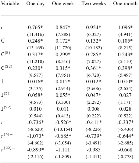
The results of the estimation of the LHAR-CJ on the S&P500 sample from January

18

1990 to February 2009, withh= 1,5,10,22are reported in Table 1.1, together with

19

their statistical significance, evaluated with the Newey-West robust t-statistic with44

20

lags.

21

As usual, all the coefficients of the three continuous volatility components are

22

positive and highly significant. We observe that the coefficient measuring the impact

23

of monthly volatility on future daily volatility (i.e. 0.203) is more than twice as big

24

as the one of daily volatility on future monthly volatility (i.e. 0.105). This finding

25

is consistent with the hierarchical asymmetric propagation of the volatility cascade

26

formalized in Section 1.3.

27

A similar hierarchical structure, although less pronounced, is present in the

im-28

pact of jumps on future volatility. The daily and weekly jump components remain

29

highly significant and positive especially when modelling realized volatility at short

30

horizons. In addition, their impact declines when the frequency at which RV is

31

modelled declines. The jumps aggregated at the monthly level, however, turn out to

32

be insignificant on the considered data set.

33

Interestingly, estimation results for model (1.17) reveal the strong significance

34

(with the economically expected negative sign) of the negative returns at (almost) all

35

frequencies, which unveils the presence of a heterogeneous structure in the leverage

36

effect as well. In fact, the daily volatility is significantly affected, not only by the

37

daily negative return of the day before (the well know leverage effect) but also of

38

the week and of the month before. This result suggests that the market aggregates

39

S&P500 LHAR in-sample regression

Variable One day One week Two weeks One month

c 0.765* 0.847* 0.954* 1.096* (11.416) (7.888) (6.327) (4.941)

C 0.248* 0.172* 0.132* 0.105*

(13.169) (11.720) (10.182) (8.215)

C(5) 0.317* 0.299* 0.285* 0.243* (11.210) (8.516) (7.027) (5.110)

C(22) 0.230* 0.315* 0.361* 0.398* (8.577) (7.951) (6.720) (5.497)

J _{0.016* 0.012* 0.012* 0.010*}

(3.135) (2.914) (3.606) (2.654)

J(5) 0.058* 0.055* 0.047* 0.027

(4.573) (3.330) (2.282) (1.171)

J(22) 0.010 0.011 0.008 0.028

(0.544) (0.413) (0.222) (0.522)

r− _{-0.736* -0.526* -0.411* -0.337*} (-8.620) (-10.154) (-8.226) (-5.436)

r(5)− _{-1.070* -0.685* -0.739* -0.644*} (-4.602) (-3.054) (-3.491) (-2.685)

r(22)− _{-0.899* -1.111 -0.985 -0.668} (-2.116) (-1.809) (-1.411) (-0.778)

Table 1.1 OLS estimates of the LHAR-CJ model (1.17), for S&P500 futures from January 1990 to February 2009, (4,766observations). The LHAR-CJ model is estimated withh= 1(one day),h= 5(one week),h= 10(two weeks) andh= 22

APPLICATIONS 17

information at the daily, weekly and monthly levels and reacts to shocks happening

1

at these three levels/frequencies. These findings thus further confirm the views of the

2

Heterogeneous Market Hypothesis.

3

To evaluate the performance of the LHAR-CJ model, we compare it with the

4

standard HAR (with only heterogeneous volatility) and the HAR-CJ model (with

5

heterogeneous jumps) on the basis of a genuine out-of-sample analysis. For the

6

out-of-sample forecast ofVbton the[t, t+h]interval we keep the same forecasting

7

horizons (one day, one week, two weeks and one month) and re-estimate the model

8

at each day t on a moving window of length 2500 days. Table 1.2 reports the

9

out-of-sample forecasts of the different models evaluated on the basis of the R2

10

of Mincer-Zarnowitz forecasting regressions and the Diebold-Mariano test for the

11

out-of-sample Root Mean Square Error (RMSE).13

12

The superiority of the HAR-CJ model over the HAR model is mild, since it has

13

to be ascribed preeminently to days which follow a jump, and thus on a very small

14

sample; conditioning on days following the occurrence of a jump would show a

15

sharper improvement (as shown in [38]). However, the superiority of the LHAR-CJ

16

model at all horizons, with respect to the HAR (and the HAR-CJ model) is much

17

stronger, validating the importance of including both the heterogeneous leverage

18

effects and jumps in the forecasting model.

19

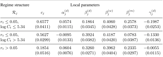
In the second part of our empirical analysis, we estimate the Tree HAR-CJ model

20

introduced in (1.19) to investigate whether additional non-linear effects are present

21

in the dynamics of the S&P500 futures volatilities on the top of the leverage effect

22

and whether the explicit modeling of structural breaks and regime-shifts is able to

23

improve the accuracy of the estimates and forecasts. To simplify the interpretations

24

and reduce the number of parameters in the model, we assume that the cascade is

25

present only in the volatility continuous componentCt(i.e. we set the parameters

26

α(jw,m) andγ

(w,m)

j , j = 1, . . . , k, to zero). Estimated coefficients, as well as the

27

estimated regimes, are reported in Table 1.3 forh = 1. Classical model-based

28

bootstrapped standard errors are given in parentheses.

29

Table 1.3 shows that almost all coefficients in the local dynamics of realized

30

volatilities are highly significant, with a couple of interesting exceptions. As

dis-31

cussed previously, the leverage effect is found to be the most important asymmetry

32

and yields the first binary split in the procedure. The optimal threshold is found

33

to be around zero, highlighting the different reaction of realized volatilities to past

34

positive and negative S&P 500 returns. A second relevant non-linear behavior of

35

realized volatility dynamics is found in response to past low and moderate vs. high

36

(continuous part) volatilities when past S&P 500 returns are negative. In fact, the

37

threshold valued2 = 5.34corresponds to the70%quantile of the estimatedlogCt

38

series.

39

In these three regimes, local volatility dynamics show significant differences. In

40

particular, it is worth mentioning the following two results: First, past lagged S&P

41

S&P500 out-of-sample performances

Variable One day One week Two weeks One month

HAR 0.8073 0.8351 0.8162 0.7573

HAR-CJ 0.8107 0.8397 0.8188 0.7597 (1.994) (1.808) (0.835) (0.115)

LHAR-CJ 0.8238 0.8487 0.8279 0.7651 (4.663) (2.854) (2.023) (1.169)

Table 1.2 R2of Mincer-Zarnowitz regressions for out-of-sample forecasts for horizonsh= 1(one day),h= 5(one week),h= 10(two weeks) andh= 22(one month) of the S&P500 from January 1990 to February 2009 (4,766 observations, the first 2500 observations are used to initialize the models). The forecasting models are the standard HAR, the HAR-CJ and the LHAR-CJ model. In parentheses is reported the Diebold-Mariano test for the out-of-sample RMSE with respect to the standard HAR model.

Tree HAR-CJ estimates and regimes

Regime structure Local parameters

Rj cj α(

d)

j β

(d)

j β

(w)

j β

(m)

j γ

(d)

j

rt≤0.05, 0.6577 0.0574 0.1864 0.4060 0.2578 −0.1987 logCt≤5.34 (0.0411) (0.0115) (0.0345) (0.0428) (0.0373) (0.0253)

rt≤0.05, 0.5627 −0.0095 0.3924 0.4187 0.0783 −0.1330 logCt>5.34 (0.0299) (0.0133) (0.0382) (0.0420) (0.0387) (0.0136)

rt>0.05 0.1854 0.0604 0.3260 0.3962 0.2335 −0.0055 (0.0516) (0.0076) (0.0271) (0.0404) (0.0297) (0.0115)

CONCLUDING REMARKS AND AREAS FOR FUTURE RESEARCH 19

500 returns are significant only in the regimes where they are negative, yielding to

1

an increase in the realized volatilities. When past lagged S&P 500 returns are

posi-2

tive (last regime) their impact in estimating future volatility dynamics is negligible.

3

Second, the impact of jumps highly changes depending on the regime in which they

4

occur: it is positive and significant in regimes characterized by (somehow) stable

5

financial markets (regimes 1 and 3), yielding to an increase of realized volatility.

6

By contrast, in times of market turbulence (measured by past negative returns and

7

high past volatilities), jumps are found to have no particular impact in driving future

8

realized volatility dynamics. These interesting results confirm and extend previous

9

empirical findings shown in this section.

10

Similarly to what has been shown above for the LHAR-CJ model, in a preliminary

11

series of forecasting experiments forhequal to one, the Tree HAR-CJ model has

12

been found to be able to significantly improve the out-of-sample performance of the

13

classical HAR and HAR-CJ models. A more detailed and complete investigation

14

of how the introduction of regimes (threshold-based or of a Markovian type) may

15

improve predictions in a general HAR setting is left for the future.

16

1.7 CONCLUDING REMARKS AND AREAS FOR FUTURE RESEARCH

17

By projecting a dynamic process on its own past values aggregated over different time

18

horizons, the HAR model is a general and flexible approach to fit the autocorrelation

19

function of any persistent process in a very simple and tractable way. In this chapter

20

we have briefly surveyed the nature, construction, and properties of the HAR class

21

of models for realized volatility estimation and prediction. We discussed some

22

of the extensions of the standard HAR model that have been recently proposed to

23

explicitly take into account the predictive power of jumps, leverage effects, and other

24

non-linearities (i.e. structural breaks and regime switches driven by the different

25

sources acting on the financial market) for the time-varying dynamics of realized

26

volatilities. We also reviewed some recent studies generalizing the HAR model

27

for predicting univariate realized volatilities to the multivariate setting of realized

28

covariance matrices. This is a fast-growing field and the list of references will no

29

doubt need updating in the near future.

30

In our review of the extant literature on HAR models a number of topics stand

31

out as possible avenues for future research. The most obvious, and perhaps difficult,

32

is to generalize the univariate flexible HAR model with jumps, leverage effects,

33

and other non-linear behaviors due to regime changes to the multivariate context.

34

Existing models do not take these effects into account and are not well-designed

35

to deal with (possibly) high-dimensional realized covariance matrices. What is

36

needed are flexible yet parsimonious multivariate HAR-type extensions that remain

37

computationally feasible in large dimensions. This task may be accomplished using

38

recent techniques coming from the computational statistics community, similar to

39

what was done ten years ago in [6] for the estimation of a flexible volatility matrix in

40

a multivariate GARCH setting.

REFERENCES

1

1. Y. A¨ıt-Sahalia and J. Jacod. Testing for jumps in a discretely observed process. Annals

2

of Statistics, 37:184–222, 2009.

3

2. Y. A¨ıt-Sahalia and L. Mancini. Out of sample forecasts of quadratic variation. Journal of

4

Econometrics, 147(1):17–33, 2008.

5

3. T. Andersen, T. Bollerslev, and F. X. Diebold. Roughing it up: Including jump components

6

in the measurement, modeling and forecasting of return volatility. Review of Economics

7

and Statistics, 89:701–720, 2007.

8

4. A. Arneodo, J.F. Muzy, and D. Sornette. Casual cascade in stock market from the

9

"infrared" to the "ultraviolet". European Physical Journal B, 2:277, 1998.

10

5. F. Audrino and P. B¨uhlmann. Tree-structured garch models. Journal of the Royal

11

Statistical Society, Series B, 63:727–744, 2001.

12

6. F. Audrino and P. B¨uhlmann. Volatility estimation with functional gradient descent for

13

very high-dimensional financial time series. Journal of Computational Finance, 6(3):1–

14

26, 2003.

15

7. F. Audrino and F. Corsi. Modeling tick-by-tick realized correlations. Computational

16

Statistics & Data Analysis, 54:2373–2383, 2010.

17

8. F. Audrino and F. Trojani. Estimating and predicting multivariate volatility regimes in

18

global stock markets. Journal of Applied Econometrics, 21:345–369, 2006.

19

9. F.M. Bandi and J.R. Russell. Realized covariation, realized beta and microstructure noise.

20

Unpublished paper, Graduate School of Business, University of Chicago, 2005.

21

10. A. Banerjee and G. Urga. Modelling structural breaks, long memory and stock market

22

volatility: An overview. Journal of Econometrics, 129(1-2):1–34, 2005.

23

11. O. E. Barndorff-Nielsen, P. R. Hansen, A. Lunde, and N. Shephard. Multivariate realised

24

kernels: Consistent positive semi-definite estimators of the covariation of equity prices

25

with noise and non-synchronous trading. Working Paper Series, 2010.

26

12. O. E. Barndorff-Nielsen and N. Shephard. Power and bipower variation with stochastic

27

volatility and jumps. Journal of Financial Econometrics, 2:1–48, 2004.

28

13. O.E. Barndorff-Nielsen, P.R. Hansen, A. Lunde, and N. Shephard. Designing realized

29

kernels to measure the ex post variation of equity prices in the presence of noise.

Econo-30

metrica, 76(6):1481–1536, 2008.

31

14. O.E. Barndorff-Nielsen and N. Shephard. Non-Gaussian Ornstein–Uhlenbeck-based

32

models and some of their uses in financial economics. Journal of the Royal

Statisti-33

cal Society: Series B (Statistical Methodology), 63(2):167–241, 2001.

34

15. O.E. Barndorff-Nielsen and N. Shephard. Measuring the impact of jumps in multivariate

35

price processes using bipower covariation. 2005.

36

16. D. Bates. Post-’87 crash fears in the S&P 500 futures option market. Journal of

Econo-37

metrics, 94:181–238, 2000.

38

17. G.H. Bauer and K. Vorkink. Forecasting multivariate realized stock market volatility.

39

Journal of Econometrics, 2010.

40

18. S. Bianco, F. Corsi, and R. Ren`o. Intraday LeBaron effects. Proceedings of the National

41

Academy of Science of the USA, 106:11439–11443, 2009.

REFERENCES 21

19. T. Bollerslev, J. Litvinova, and G. Tauchen. Leverage and volatility feedback effects in

1

high-frequency data. Journal of Financial Econometrics, 4(3):353, 2006.

2

20. T Bollerslev, G Tauchen, and H Zhou. Expected stock returns and variance risk premia.

3

Review of Financial Studies, 22(11):4463–4492, 2008.

4

21. T. Bollerslev and J.H. Wright. Volatility forecasting, high-frequency data, and frequency

5

domain inference. Review of Economics and Statistics, 83:596–602, 2001.

6

22. T. Bollerslev and B. Y. B. Zhang. Measuring and modeling systematic risk in factor

7

pricing models using high-frequency data. Journal of Empirical Finance, 10(5):533–558,

8

2003.

9

23. M. Bonato, M. Caporin, and A. Ranaldo. Forecasting realized (co)variances with a block

10

structure Wishart autoregressive model. Working Papers, 2009.

11

24. K. Boudt, C. Croux, and S. Laurent. Outlyingness weighted quadratic covariation.

Work-12

ing Paper, 2008.

13

25. L. Breiman, J. Friedman, C. J. Stone, and Richard A. Olshen. Classification and regression

14

trees. Chapman & Hall/CRC, 1984.

15

26. L.E. Calvet and A.J. Fisher. How to forecast long-run volatility: Regime switching and

16

the estimation of multifractal processes. Journal of Financial Econometrics, 2(1):49–83,

17

2004.

18

27. J. Y. Campbell and L. Hentschel. No news is good news: a asymmetric model of changing

19

volatility in stock returns. Journal of Financial Economics, 31:281–318, 1992.

20

28. R. Chiriac and V. Voev. Modelling and forecasting multivariate realized volatility. Journal

21

of Applied Econometrics, 2010.

22

29. K. Christensen, R. Oomen, and M. Podolskij. Realised quantile-based estimation of the

23

integrated variance. Journal of Econometrics, 159(1):74–98, 2010.

24

30. A. Christie. The stochastic behavior of common stock variances: value, leverage and

25

interest rate effects. Journal of Financial Economics, 10:407–432, 1982.

26

31. M.P. Clements, A.B. Galv˜ao, and J.H. Kim. Quantile forecasts of daily exchange rate

27

returns from forecasts of realized volatility. Journal of Empirical Finance, 15(4):729–750,

28

2008.

29

32. K. Cohen, G. A. Hawawini, S. F. Maier, R. Schwartz R., and D. Whitcomb D. Friction in

30

the trading process and the estimation of systematic risk. Journal of Financial Economics,

31

12:263–278, 1983.

32

33. F. Comte and E. Renault. Long memory in continuous-time stochastic volatility models.

33

Mathematical Finance, 8(4):291–323, 1998.

34

34. F. Corsi. A simple approximate long-memory model of realized volatility. Journal of

35

Financial Econometrics, 7:174–196, 2009.

36

35. F. Corsi and F. Audrino. Realized covariance tick-by-tick in presence of rounded time

37

stamps and general microstructure effects. Unpublished manuscript, University of St.

38

Gallen, 2008.

39

36. F. Corsi, D. La Vecchia, and N. Fusari. Realizing smiles: Pricing options with realized

40

volatility. Working Paper, 2010.

41

37. F. Corsi, S. Mittnik, C. Pigorsch, and U. Pigorsch. The volatility of realized volatility.

42

Econometric Reviews, 27(1-3):1–33, 2008.

38. F. Corsi, D. Pirino, and R. Ren`o. Threshold bipower variation and the impact of jumps

1

on volatility forecasting. Journal of Econometrics, 159:276–288, 2010.

2

39. F. Corsi and R. Renò. Discrete-time volatility forecasting with persistent leverage effect

3

and the link with continuous-time volatility modeling. Working Paper, 2010.

4

40. G. Curci and F. Corsi. Discrete sine transform for multi-scales realized volatility measures.

5

Quantitative Finance, 2010. Forthcoming.

6

41. M.M. Dacorogna, U.A. M¨uller, R.D. Davé, R.B. Olsen, and O.V. Pictet. Modelling

short-7

term volatility with garch and harch models. In "Nonlinear Modelling of High Frequency

8

Financial Time Series", pages 161–76, 1998. edited by C. Dunis and B. Zhou, John Wiley,

9

Chichester.

10

42. F. De Jong and T. Nijman. High frequency analysis of lead-lag relationships between

11

financial markets. Journal of Empirical Finance, 4(2-3):259–277, 1997.

12

43. R.F. Engle and G.G.J. Lee. A permanent and transitory component model of stock return

13

volatility. In R.F. Engle and H. White, editors, Cointegration, Causality, and Forecasting:

14

A Festschrift in Honor of Clive WJ Granger, pages 475–497. Oxford University Press,

15

Oxford, 1999.

16

44. T. Epps. Comovements in stock prices in the very short run. Journal of the American

17

Statistical Association, 74:291–298, 1979.

18

45. L. Forsberg and E. Ghysels. Why do absolute returns predict volatility so well? Journal

19

of Financial Econometrics, 5:31–67, 2007.

20

46. C. Francq and J.M. Zakoian. Bartlett’s formula for a general class of nonlinear processes.

21

Journal of Time Series Analysis, 30(4):449–465, 2009.

22

47. E. Ghysels, P. Santa-Clara, and R. Valkanov. Predicting volatility: getting the most out of

23

return data sampled at different frequencies. Journal of Econometrics, 131(1-2):59–95,

24

2006.

25

48. E. Ghysels, A. Sinko, and R. Valkanov. Midas regressions: Further results and new

26

directions. Econometric Reviews, 26:53–90, 2006.

27

49. R. Giacomini and H. White. Tests of conditional predictive ability. Econometrica,

28

74(6):1545–1578, 2006.

29

50. L. Glosten, R. Jagannathan, and D. Runkle. On the relation between the expected value of

30

the volatility of the nominal excess return on stocks. Journal of Finance, 48:1779–1801,

31

1989.

32

51. S. Gonc¸alves and N. Meddahi. Box-Cox transforms for realized volatility. Journal of

33

Econometrics, 160(1):129–144, 2011.

34

52. C. Granger. Long memory relationships and the aggregation of dynamic models. Journal

35

of Econometrics, 14:227–238, 1980.

36

53. J.E. Griffin and R.C.A. Oomen. Covariance measurement in the presence of

non-37

synchronous trading and market microstructure noise. Journal of Econometrics, 160(1):58–

38

68, 2011.

39

54. T. Hayashi and N. Yoshida. On covariance estimation of non-synchronously observed

40

diffusion processes. Bernoulli, 11(2):359, 2005.

41

55. J. Jacod, Y. Li, P.A. Mykland, M. Podolskij, and M. Vetter. Microstructure noise in the

42

continuous case: The pre-averaging approach. Stochastic Processes and their

Applica-43

tions, 119(7):2249–2276, 2009.

REFERENCES 23

56. G.J. Jiang and R.C.A. Oomen. Testing for jumps when asset prices are observed with

1

noise–a "swap variance" approach. Journal of Econometrics, 144(2):352–370, 2008.

2

57. X. Jin and J. Maheu. Modelling realized covariances and returns. Working Papers, 2010.

3

58. B. LeBaron. Stochastic volatility as a simple generator of financial power-laws and long

4

memory. Quantitative Finance, 1:62131, 2001.

5

59. S.S. Lee and P.A. Mykland. Jumps in financial markets: A new nonparametric test and

6

jump dynamics. Review of Financial studies, 21(6):2535, 2008.

7

60. A. Lo and W. Andrew. An econometric analysis of nonsynchronous trading. Journal of

8

Econometrics, 45(1-2):181–211, 1990.

9

61. P. Lynch and G. Zumbach. Market heterogeneities and the causal structure of volatility.

10

Quantitative Finance, 3(4):320–331, 2003.

11

62. C. Mancini. Non-parametric threshold estimation for models with stochastic diffusion

12

coefficient and jumps. Scandinavian Journal of Statistics, 36(2):270–296, 2009.

13

63. C. Mancini and R. Ren`o. Threshold estimation of Markov models with jumps and interest

14

rate modeling. Journal of Econometrics, 160(1):77–92, 2011.

15

64. M.E. Mancino and S. Sanfelici. Estimating covariance via Fourier method in the presence

16

of asynchronous trading and microstructure noise. Journal of Financial Econometrics,

17

2010. Forthcoming.

18

65. A. McAleer and M.C. Medeiros. A multiple regime smooth transition heterogeneous

19

autoregressive model for long memory and asymmetries. Journal of Econometrics,

20

147:104–119, 2008.

21

66. U. Muller, M. Dacorogna, R. Dav´e, R. Olsen, O. Pictet, and J. von Weizsacker. Volatilities

22

of different time resolutions - analyzing the dynamics of market components. Journal of

23

Empirical Finance, 4:213–239, 1997.

24

67. A. Palandri. Consistent realized covariance for asynchronous observations contaminated

25

by market microstructure noise. Unpublished Manuscript, 2006.

26

68. R. Ren`o. A closer look at the Epps effect. International Journal of Theoretical and

27

Applied Finance, 6(1):87–102, 2003.

28

69. M. Scharth and M.C. Medeiros. Asymmetric effects and long memory in the volatility of

29

dow jones stocks. International Journal of Forecasting, 25:304–327, 2009.

30

70. M. Scholes and J. Williams. Estimating betas from nonsynchronous data. Journal of

31

Financial Economics, 5:181–212, 1977.

32

71. K. Sheppard. Realized covariance and scrambling. Unpublished Manuscript, 2006.

33

72. V. Voev and A. Lunde. Integrated covariance estimation using high-frequency data in the

34

presence of noise. Journal of Financial Econometrics, 5:68–104, 2007.

35

73. L. Zhang. Efficient estimation of stochastic volatility using noisy observations: a

multi-36

scale approach. Bernoulli, 12(6):1019–1043, 2006.

37

74. L. Zhang, P. A. Mykland, and Y. A¨ıt-Sahalia. A tale of two time scales: Determining

38

integrated volatility with noisy high-frequency data. Journal of the American Statistical

39

Association, 100:1394–1411, 2005.