A new flat shell finite element for the linear analysis of thin shell structures

City, University of London Institutional Repository

Citation

: Hamadi, D., Ayoub, A. & Abdelhafid, O. (2016). A new flat shell finite element for

This is the accepted version of the paper.

This version of the publication may differ from the final published

version.

Permanent repository link:

Link to published version

: http://dx.doi.org/10.1080/17797179.2016.1153401

Copyright and reuse:

City Research Online aims to make research

outputs of City, University of London available to a wider audience.

Copyright and Moral Rights remain with the author(s) and/or copyright

holders. URLs from City Research Online may be freely distributed and

linked to.

City Research Online: http://openaccess.city.ac.uk/ [email protected]

A NEW FLAT SHELL FINITE ELEMENT FOR THE LINEAR

ANALYSIS OF THIN SHELL STRUCTURES

Djamal Hamadi

, Ashraf Ayoub

, and Ounis Abdelhafid

a, c

Civil Engineering and Hydraulics Department, Faculty of Sciences and Technology, Biskra University, B.P.145, 07000 Biskra – Algeria

b

Corresponding author; School of Mathematics, Computer Science, and Engineering, City University London, Northampton Square, London EC1V 0HB, UK., Phone: 44(0) 20 7040 8912, Email:

A NEW FLAT SHELL FINITE ELEMENT FOR THE LINEAR

ANALYSIS OF THIN SHELL STRUCTURES

Abstract

In this paper, a new rectangular flat shell element denoted 'ACM_RSBE5' is presented. The new element is obtained by superposition of the new strain-based membrane element 'RSBE5' and the well-known plate bending element 'ACM'. The element can be used for the analysis of any type of thin shell structures; even if the geometry is irregular. Comparison with other types of shell elements is performed using a series of standard test problems. A correlation study with an experimentally tested aluminum shell is also conducted. The new shell element proved to have a fast rate of convergence and to provide accurate results.

Keywords: Flat shell element; thin shell; strain based approach; static condensation.

1. Introduction

Analytical solutions of practical thin shell structures, particularly those with irregular geometrical shapes, are complex and thus a resort to numerical methods when analyzing them becomes essential. Early work aimed to study shells of revolution in which closed ring shell segments are used [e.g. Jones and Strome, 1966]. The formulation of flat elements [Zienkiewics, 1977] and curved rectangular elements [Corner and Brebbia, 1967] followed. These elements are based on assumed polynomial displacements with linear representation of the in-plane displacements. These elements were found to have a slow rate of convergence, thus the development of high order elements received more attention. Meanwhile, a simple strain-based alternative approach was proposed by Ashwell and Sabir (1972). In this approach, the exact terms representing all rigid body modes and displacement functions corresponding to the element strains are determined by assuming independent strain functions that satisfy the compatibility equations. This approach was used successfully by Sabir and his co-workers (1982, 1985, 1990, 1997) and Mousa and Sabir (1994) to analyze cylindrical, hyperbolic and conical shell structures. These elements in general proved to have a faster convergence rate compared to other models available in the literature. On the other hand, a family of enhanced strain elements, originally developed by Simo and Rifai (1990), were proposed. These include one-point quadrature elements developed by Cardoso et al. (2006, 2008), 4-node exact geometry element proposed by Kulikov and Plotnikova (2010), the improved solid-shell elements of Abed-Meraim and Combescure (2009) using physical stabilization, of Reese (2007) using hourglass stabilization, and of Schwarze and Reese (2009) using reduced integration.

of freedom at each node and proved to yield accurate results even when using very few finite elements. We note here that most of the above efficient elements are formulated with the appropriate coordinates of the geometrical shape of the structures. Generally, for design purposes, shell structures are constructed with very complicated geometrical shapes and elements, such as folded plates and edge beams. Additional geometrical problems arise, such as when openings, anisotropy, or variation of thickness, are present. However, for practical purposes the flat element approximation gives generally adequate results and permits easy coupling with edge beams and rib members, a capability usually not present in curved element formulations [Zienkiewics and Taylor, 2000]. In flat shell elements, the coupling between membrane and bending action is accounted for at the integration points due to the varying orientation of the element. For practical analysis of shell structures, such flat plate element assumption is typically acceptable, and has the advantage of ease of modeling with reasonable accuracy. Further, because the membrane and bending stresses within an element are decoupled it is easy to understand and control the behaviour of such elements [Hartmann and Kats, 2007]. In this case, the behaviour of a continuously curved surface is represented by a surface made up of small flat elements. Intuitively, as the size of the subdivision decreases it would seem that convergence must occur as discussed by Zienkiewics and Taylor (2000).

In this paper, a new flat shell element is proposed and is denoted as (ACM_ RSBE5). The element is developed by superposition of the new rectangular membrane element R4SBE5 based on the strain approach and the well-known plate bending element ACM discussed in detail in Adini and Clough (1961) and Melosh (1963). The element is characterized by its simplicity compared to existing elements, without compromising its numerical robustness. The stiffness matrix of the new shell element is obtained by combining the two independent membrane and bending stiffness matrices. The displacement field for the strain based membrane element RSBE5 used to construct the flat shell element fully satisfies the equilibrium equations in addition to the compatibility equations. Also, the technique of static condensation of a middle node and the new analytical integration employed in the formulation are the new additions that distinguish this element from other flat shell elements presented in previously published works [e.g. Ashwell and Sabir, 1972; Sabir and Lock, 1972; Belarbi, 2000; Batoz and Dhatt, 1992].

Ashwell and Sabir (1972) developed a cylindrical shell finite element. The element is a rectangular one, having twenty degrees of freedom. It uses only external geometrical nodal displacement, three linear displacements and two rotations; and its formulation is based on strain functions using polar coordinates. The effectiveness of this element has been tested by using it for the analysis of pinched cylinder shell and barrel vault problems. The results showed rapid convergence for displacement. Sabir and Lock (1972) also developed a curved cylindrical shell finite element. They used the standard finite element approach for the formulation adopted by Cantin and Clough (1968), but removed the nodal degrees wxy and included terms containing trigonometrical functions to develop a rectangular cylindrical shell element with 4 nodes and 5 dof/node; which leads to a 20x20 element stiffness matrix. This element is found to converge more rapidly than the Cantin and Clough’s model for both symmetrical and unsymmetrical loading conditions. The applications of the elements developed by Sabir and his co-workers are limited to cylindrical shell structures, while the proposed element is a flat shell which can be used for the analysis of general-shape shell structures. The present element contains a middle node to enrich the displacement field that is subsequently condensed out. The element also uses an analytical integration to evaluate the stiffness matrix.

(Melosh, 1963). The SBQ4 element (Strain Based Quadrilateral element with 4-node) is based on the strain approach, with three degrees of freedom per node including a drilling rotation. The membrane and bending stiffness matrix is obtained by using an analytical integration. This element was examined with three essentials shell tests and the results obtained are compared with those of the proposed 'ACM_RSBE5 in addition to the reference solution. The membrane element SBQ4 contains 4 nodes and 3DOF/node (2 translations and one drilling rotation); but the present element RSBE5 contains 5 nodes: 4 corner nodes and a middle node with 2 translations/node.

Batoz and Dhatt (1992) formulated a set of quadrilateral shell elements based on displacement formulations ; among them Q4 24 and DKQ24. The first element is based on the Mindlin theory formulation, having four nodes with six degrees of freedom per node and using numerical integration. The second is a flat shell element obtained by superposition of the well-known classical quadrilateral membrane element Q4 and the plate bending element DKQ (Discrete Kirchhoff quadrilateral element with 4 nodes and 3 dof per node). The DKQ24 element is based on Kirchhoff theory with four nodes and six degrees of freedom per node. These two elements are applied to the numerical analysis of Scordelis-Lo (1969) roof test presented in the numerical section in this paper. The results obtained are compared with the reference solutions for both shallow and deep shell theory, in addition to the new formulated element 'ACM_RSBE5' and the flat shell element ACM-SBQ4. We should mention here that the analytical integration technique is used to compute the element stiffness matrices for both elements 'ACM_RSBE5' and ACM-SBQ4. The improved results obtained from the numerical simulations clearly prove the advantages of the proposed element.

In the next section, the formulation of the new element ACM_RSBE5 is presented, followed by standard test problems to evaluate its convergence compared to other quadrilateral shell elements present in the literature. Finally, a correlation study with an experimentally tested elliptical paraboloid shell structure subjected to a uniformly distributed load is presented and the results are discussed.

2. Construction of the New Flat Shell Element ACM_RSBE5

The proposed rectangular shell element is obtained by the superposition of the new formulated element "RSBE5" based on the strain approach and described in the next section, and the ACM standard plate bending element. The stiffness matrix of the shell element ACM_ RSBE5 is calculated through analytical integration of the membrane and bending stiffness matrices.

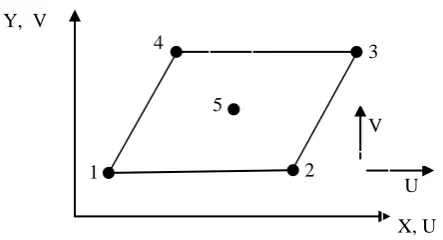
2.1. Formulation of the New Membrane Element "RSBE5"

Figure 1 shows the geometry and nodal displacements of the “RSBE5” element (Rectangular Strain Based Element with 5 nodes). The degrees of freedom at each node (i) are denoted U_iand V_i for the horizontal and vertical displacements respectively. The element was developed by Hamadi (2006) and has four nodes at the corner in addition to an internal node, each having two degrees of freedom (d.o.f). Through the introduction of an additional internal node, the element has proven to be more accurate, even though it requires static condensation following the approach of Bathe and Wilson (1976).

[Fig. 1]

The strain components at any point in the Cartesian coordinate system are expressed in terms of the displacements U and V as follow:

y = V,y (1b)

xy = U,y+ V,x (1c)

If the strains given by equations (1) are equal to zero, the integration of equations (1) leads to expressions of the form:

U = a1 - a3 y

(2a) V = a2 + a3 x

(2b)

Equations (2) represent the displacement field in terms of its three rigid body displacements. The strains in equation (1) cannot be considered independent since they must satisfy the compatibility equation. This equation can be obtained by eliminating U, V from equation (1), hence:

0 2 2 2 2 2    y x x y xy y x           (3)

Equation (2) represents the three components of the rigid body displacements through three independent constants (a1, a2, a3). Thus seven additional constants (a4, a5… a10) are needed to express the displacements due to straining of the element. These seven independent constants are used to describe the strains as follow:

4 5 9

6 7 10

5 7 8 9 10

a a a

a a a

a R a R + a a a

x y xy

y x

x y

x y Hy Hx

             _{    }  (4) With:

 

 

1 1 v H R v v    

The strains given by equations (4) satisfy both the compatibility equation (3) and the two-dimensional equilibrium equations (5a) and (5b):

  0

y x xy x     (5a) 0   x y xy y     (5b)

By integrating equations (4), the displacements are evaluated as follow:

U = a4 x+ a5 xy - a7 y2 (R +1)/2+ a8 y/2 + a9 (x2 – H y2)/2

(6a)

V = - a5 x2(R + 1)/2+ a6 y+ a7 xy + a8 x/2 + a10 (y2 – Hx2)/2 _(6b)









2

2 2

1 3 4 5 7 8 9

2

2 2

2 3 5 6 7 8 10

1 2 1

2

1

a a a a a a a ( )

2 2

1

a +a a a a a +a ( )

2 2

y R

x R

y

U y x xy x Hy

x

V x y xy y Hx

                      (7)

The stiffness matrix is then calculated from the well-known expression:

[Ke] = [A-1 ]T [K0 ] [A-1 ] (8a)

where [K0] =

    

S T

.



 

0 0 0 0 0 1

y x

Q x y

xR yR Hy Hx

               (9)

[D] =       

D11 D12 0

D12 D22 0

0 0 D33

is the usual constitutive matrix





11 22 1 E D D   

 ;





. 12 1 E D   

 ; 33 2 1 

E D







For [A] and [K0] see Appendices A and B.

At the end of the state determination, the 2 additional middle dofs are condensed out. The evaluation of the integral in Eq. (8b) follows the approach of Hamadi and Belarbi (2006) using an exact and not reduced analytical integration. Such an approach resolves numerical problems associated with geometrical distortions of the element.

2.2. Rectangular Plate Element ‘ACM’

The displacement fields of the ACM element (Fig.2) are given by the following expressions:

[Fig. 2]

W(x,y) = a1 + a2 x + a3 y+ a4 x2 + a5 xy + a6 y 2 + a7 x3 + a8 x2y

+ a9 xy2 + a10 y3 + a11 x3y + a12 xy3

x = -(a3+ a5 x +2 a6 y+ a8 x

2

+ 2a9 xy + 3 a10 y 2 + a11 x3 +3 a12 xy2) (10)

_y = a2 + 2a4 x + a5 y+3a7 x2 + 2a8 xy + a9 y2 +3 a11 x2 y+ a12 y3

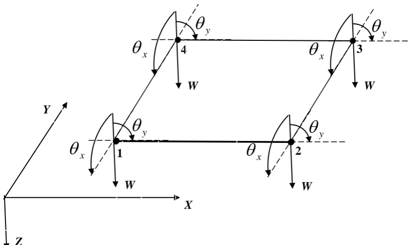
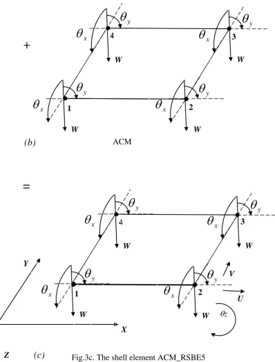
(a)

+ (b) = (c)

[Fig. 3]

3. Numerical Tests

The performanceof the formulated flat shell element is evaluated using the following popular test problems:

3.1. Clamped Cylindrical Shell

In this test problem, a clamped cylindrical shell (Fig.4 a) is evaluated. This test of thin shells (R/h=100) is considered by many researchers as a severe test. It makes it possible to examine the aptitude of shell elements to simulate complicated membrane state problems dominated by bending. The dimensions, material properties, and loading conditions are shown in Fig.4. Due to symmetry, only 1/8 of the shell (region ABCD) is considered in the finite element idealisation (Fig.4 b).

[Fig. 4]

The results obtained for different meshes for both, the proposed ACM_RSBE5 and the ACM_SBQ4 of Belarbi (2000), are presented in Tables 1 and 2.

[Tables 1-2]

The numerical results are compared to the analytical solution based on thin shell theories (R/h=100), and given below by Flugge and Fosberge (1966) and Lindberg et al. (1969):

WC = -WC Eh/P = 164.24 deflection under load P at point C only

VD = -VD Eh/P = 4.11 deflection in the Y direction

Table 1 also summarizes the solution time used in the analysis of the clamped cylindrical shell with different meshes. The processor machine used has the following properties: Intel(R) Core(TM) i3-2330M [email protected] GHZ RAM: 4.00Go

et al. (2013), its performance is relatively good (0.955 as opposed to 0.979 for a mesh of 8x8).

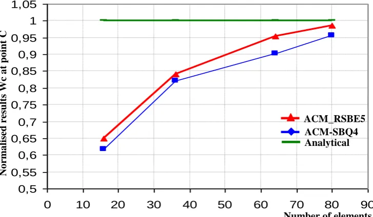
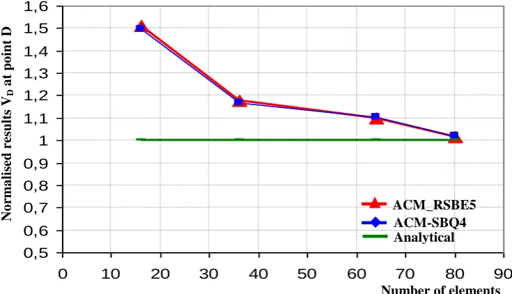
The results obtained for both deflections WC and VD for the refined mesh (20x4) of the proposed element are in good agreement with the analytical solution.

Figures 5 and 6 show the convergence curves for the results obtained from elements ACM_RSBE5 and ACM-SBQ4 for the deflections at points C and D. From the above figures, it is concluded that the ACM_RSBE5 has a good convergence rate.

[Figs. 5-6]

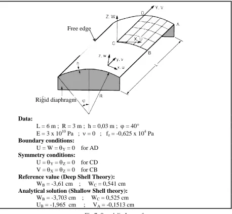
3.2. Scordelis-Lo Roof

In the next test problem, the Scordelis-Lo (1969) roof is considered. The roof structure has the geometry shown in Fig.7. The straight edges are free, while the curved edges are supported on rigid diaphragms along their plane. The geometry and material properties are given in Fig.7. Considering the symmetry of the problem, only one quarter of the roof is analysed (part ABCD). The results obtained using the proposed element ACM_RSBE5 are compared to the reference values based on the deep shell theory.

[Fig. 7]

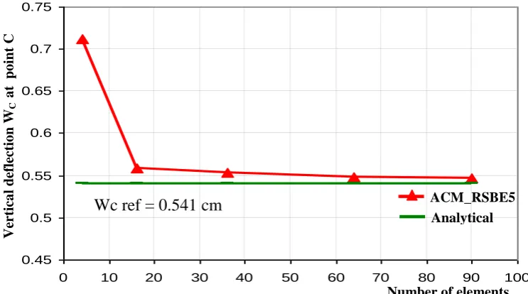
The analytical solution based on the shallow shell theory is given by Scordelis and Lo (1969), which is slightly different from the deep shell theory. The convergence curves are presented in Figs.8 and 9 for the vertical displacement at the midpoint B of the free edge and the center C of the roof.

[Figs. 8-9]

The results are also compared to several other quadrilateral shell elements, namely Q4 24, DKQ24 presented by Batoz and Dhatt (1992) and ACM-SBQ4 developed by Belarbi (2000). Figures 8, 9, 10, and 11 show the convergence curve for the deflections Wc at point C and WB at point B obtained from the quadrilateral shell elements cited above.

The above results confirm the good convergence of the new formulated shell element ACM_RSBE5.

[Figs. 8-11]

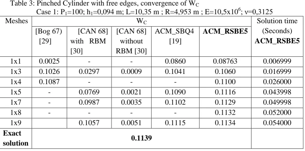
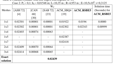
3.3. Pinched Cylinder with Free Edges

The pinched cylinder shown in Fig. 12 is one of the most common examples used in the literature to test shell elements. Indeed, since 1967 this example served as a test problem to assess the performance of new axisymmetric shell elements regarding the rapidity of convergence and especially the representation of rigid body modes. By reason of symmetry, only one-eighth of the cylinder is modeled. The symmetry conditions are imposed along AB, AD and DC (Fig.12). Two cases of cylinder thickness and applied loads are considered (h1, F1 and h2, F2).

[Fig. 12]

with the analytical solution (deep shells theory) and with other elements available in the literature; these are models: BOG (Bogner et al. 1967); CAN68 (Cantin and Clough, 1968); ASH72 (Ashwell and Sabir, 1972); and SAB72 (Sabir and Lock, 1972). The results obtained are presented in Tables 3 and 4, and the convergence curves for different elements are shown in Figs. 13 and 14.

[Tables 3-4]

[Figs. 13-14]

The results obtained and presented in Tables 3, 4 and Figs. 13 and 14 confirm the excellent performance of the formulated element ACM_RSBE5. The ACM_RSBE5 converges to deep shell solutions (to WC = - 0.1139 m for h = 0.094m and F= 100 and from WC = - 0.02439 m h = 0.01548 m) with only a few elements (9 elements for the first case and 3 elements for the second case), contrarily to the other elements and slightly better than ACM_SBQ4.

4. Experimental Investigation

A correlation study with an experimentally tested shell structure is conducted. The shell is assumed to be constructed from a perfectly elastic material. Tests on full-scale shell structures are scarce due to the associated high cost; hence the experimental work described in this study is for a small-scale specimen. The test details are described next.

4.1. Description of the Elliptical Paraboloid Shell Model (Fig.15)

The equation for the surface is written in the following manner as discussed by Beles and Soare (1975):

Z f x l f y l x x y y 1 2 2 2 2 4 4

  (11a)

2 2 2 ) ( 4 ) ( 4 y y y x x x l l y y f l l x x f

Z     (11b)

Z f x

l f y l x x y y 3 2 ₂ 2 2 1 4       

  (11c)

[Fig. 15]

The elliptical shape specimen is made of an aluminum alloy and has a constant thickness of 2 mm with a rectangular projection of 880 mm by 400 mm (Fig. 16). The material properties used are: The modulus of elasticity E = 70000 N/mm2, the Poisson ratio = 0.33. The shell is free along the long edges, and fixed on a wooden support along the short edges. Due to the double symmetry in geometry and loading, the measuring points are located on one quarter of the area of the model, at the eight points shown in Fig.17.

Eight deflections gauges capable of measuring displacements perpendicular to the surface of the shell are located under the shell. A further two deflection gauges are mounted to check for symmetry (Fig.17).

4.2. Loading

A uniform normal pressure is applied by covering the shell top surface with a pneumatic pressure bag. Four different values of loading are applied, 10, 20, 30, and 40 cm of water (in which 1 cm of water = 0.0142233 lb/ in2 equivalent to 2.5x103 N/mm2).

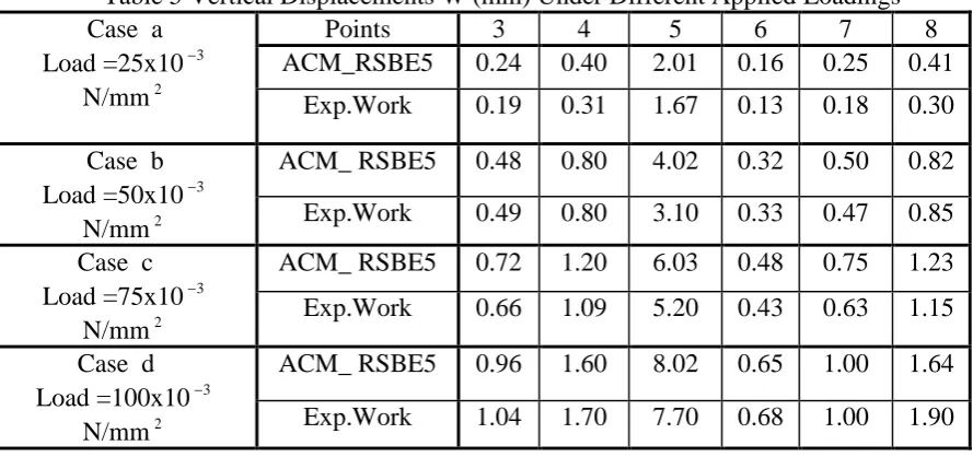
4.3 Numerical and Experimental Results

A mesh of 16x8 elements is used for the numerical analysis. The experimental and analytically computed vertical deflections for the different loading levels are presented in Table 5.

[Table 5]

4.4. Comparison between Theoretical and Experimental Results

In elastic analysis, as the loading was doubled, the deflections were doubled. This was not the case in the experimental work. This is due to a few points which could be explained as follows:

One of the main problems with the experiment was the lack of uniformity of the distributed load. The air-filled bag did not evenly distribute the pressure because loads measured at the four corners were found to be slightly different.

A further probable cause of inaccuracy was the positioning of the deflection gauges. The problem was to ensure that the gauges were perpendicular to the shell surface. Although this was easy to achieve in the central position (since it is horizontal), this was note so easily achieved near the edges where the shell surface is considerably angled.

In addition to the various experimental inaccuracies, in the theoretical analysis non deflecting support conditions are assumed, which is not strictly the case in the experiments. Finally, differences may results from other considerations. However, in general the results obtained from the finite element analysis are in reasonable agreement with those measured experimentally.

5. Conclusion

References

Abed-Meraim, F., and Combescure, A. (2007). A physically stabilized and locking-free formulation of the SHB8PS solid–shell element. European Journal of Computational Mechanics 16(8):1037–1072.

Abed–Meraim, F., Comberscure, A. (2009). An Improved Assumed Strain Solid shell Element Formulation with Physical Stabilization for Geometric Non–linear Applications and Elastic-plastic Stability Analysis. Int. Journal for Numerical Methods in Eng., 80, 1640–1686.

Abed-Meraim, F., Trinh, V., and Combescure, A. (2012). Assumed strain solid–shell formulation for the six-node finite element SHB6: evaluation on non-linear benchmark problems, European Journal of Computational Mechanics, 21:1-2, 52-71.

Abed-Meraim, F., Trinh, V., and Combescure, A. (2013). New quadratic solid–shell elements and their evaluation on linear benchmark problems. Computing 95:373–394.

Adini A. and Clough R.W. (1961). Analysis of plate bending by the finite element method. Report to the Nat. Sci. Found., U.S.A., G 7337.

Alves de Souza, R.J., Cardoso, R.P.R., Fontes Valente, R.A, Yoon, J.W., Gracio, J.J., and Jorge, R.M.N. (2005). A new one-point quadrature enhanced assumed strain (EAS) solid-shell element with multiple integration points along thickness: Part I—geometrically linear applications. Int. Journal for Numerical Methods in Eng., 62, 952–977.

Ashwell, D.G. and Sabir, A.B. (1972). A new cylindrical shell finite element based on simple independent strain functions. Int. J. Mech. Sci.; (14): 171-183.

Bathe K.J. and Wilson E.L. (1976). Numerical Methods in finite element analysis. Prentice Hall, New Jersey.

Batoz J.L., and Dhatt G. (1992). Modélisation des structures par éléments finis, Vol. 3 : coques, Eds Hermès, Paris.

Belarbi M.T. (2000). Développement de nouveaux éléments finis basés sur le modèle en déformation. Application linéaire et non linéaire. Thèse de Doctorat d’état, Université de Constantine, Algérie.

Beles, A. A. Soare, M. V. (1975). Elliptic and Hyperbolic Paraboloidal Shells Used in Construction. Bucharest, 145-146.

Bogner F.K., Fox R.L. and Schmit L.A. (1967). A cylindrical Shell Discrete Element, AIAA Journal, Vol. 5, N° 4, pp. 745-750.

Cantin G. and Clouth R.W. (1968). A curved cylindrical shell Finite Element, AIAA Journal, Vol. 6, N° 6, pp. 1057-1062.

Cardoso, R.P.R., Yoon, J.W., and Fontes Valente, R.A. (2006). A New Approach to Reduce Membrane and Transverse Shear Locking for One-point Quadrature Shell Elements: Linear Formulation. Int. Journal for Numerical Methods in Eng., 66, 214–249.

Cardoso, R.P., Yoon, J.W., Mahardika, M., Choudhry, S., Alves de Sousa, R.J., and Fontes Valente, R.A. (2008). Enhanced Assumed Strain (EAS) and Assumed Natural Strain (ANS) Methods for One-point Quadrature Solid–shell Elements. Int. Journal for Numerical Methods in Eng., 75, 156–187.

Corner JJ, Brebbia C. (1967). Stiffness matrix for shallow rectangular shell element. J. Eng. Mech., ASCE, 93(EM5): 43-65.

Djoudi, M.S and Bahai, H. (2003). A shallow shell finite element for linear and non-linear analysis of cylindrical shells. Engineering Structures, (25): 769-778.

Djoudi, M.S and Bahai, H. (2004). A cylindrical strain- based shell element for vibration analysis of shell structures. Finite Element in Analysis and Design, (40): 1947-1961. Flugge W. and Fosberge K. (1966). Point load on shallow elliptic paraboloid. J. Appl. Mech.,

Hamadi, D. (2006). "Analysis of structures by non-conforming finite elements. PhD Thesis, Civil Engineering Department, Biskra University, Algeria, pp. 130.

Hamadi, D. and Belarbi, M.T. (2006). Integration solution routine to evaluate the element stiffness matrix for distorted shapes. Asian Journal of Civil Engineering (Building and Housing), 7(5): 525 -549.

Hartmann F. and Kats C. (2007). Analysis with finite element methods. Springer.

Jones RE, Strome DR. (1966). Direct stiffness method analysis of shells of revolution utilizing curved elements. AIAA.J, 4(9): 1519-25.

Kulikov, G.M., Plotnikova, S.V. (2010). A Family of ANS Four–node Exact Geometry Shell Elements in General Convected Curvilinear Coordinates. Int. Journal for Numerical Methods in Eng., 83, 1367–1406.

Lindberg G.M., Olson M.D. and Cowper G.R. (1969). New development in the finite element analysis of shells. Q. Bull Div. Mech. Eng. and Nat. Aeronautical Establishment, National Research council of Canada, Vol. 4.

Melosh R.J., (1963). Basis of derivation of matrices for the direct stiffness method. J.AIAA, 1(N7): 1631-1637.

Mousa, A.I. and Sabir, A.B. (1994). Finite element analysis of fluted conical shell roof structures. Computational Structural Engineering in Practice, Civil Comp. press- ISRN O-948 748- 30x: 173-181.

Mousa, A.I. (1992). Triangular finite element for analysis of spherical shell structures. UWCC Publications, Internal Report, University of Wales, college Cardiff, U.K.

Mousa A.I and EL Naggar, M.H. (2007). Shallow Spherical Shell Rectangular Finite Element for Analysis of Cross Shaped Shell Roof. Electronic Journal of Structural Engineering, (7): 769-778.

Reese, S. (2007). A Large Deformation Solid–shell Concept Based on Reduced Integration with Hourglass Stabilization. Int. Journal for Numerical Methods in Eng., 69, 1671–1716. Sabir A.B. and Lock A.C. (1972). A curved cylindrical shell finite element, IJMS. Vol. 14,

pp. 125-135.

Sabir, A.B and Charchaechi, T.A. (1982). Curved rectangular and general quadrilateral shell finite elements for cylindrical shells. The Math of Finite Element and Appli., IV Academic Press: 231-239.

Sabir, A.B and Ramadhani, F. (1985). A shallow shell finite element for general shell analysis. Variation Method in Engineering, Proceedings of the 2nd International Conference, University of Southampton, England.

Sabir, A.B and Djoudi, M.S. (1990). A shallow shell triangular finite element for the analysis of hyperbolic parabolic shell roof. FEMCAD. Struct. Eng. and Optimization: 49-54. Sabir, A.B. (1997). Strain based shallow spherical shell element. Proc. Int. Conf on the Math.

Finite elements and application, Brunel University, England.

Sabir, A.B and Djoudi, M.S. (1998). A shallow shell triangular finite element for the analysis of spherical shells. Structural Analysis J.: 51-57.

Scordelis A.C. and Lo K.S. (1969). Computer analysis of cylindrical shells. J. Amer. Concrete Institute, (61): 539-561.

Simo, J.C. Rifai, M.S. (1990). A Class of Mixed Assumed Strain Methods and the Method of Incompatible Modes. Int. Journal for Numerical Methods in Eng., 29, 1595–1638.

Schwarze, M., Reese, S. (2009). A Reduced Integration Solid–shell Finite Element Based on the EAS and the ANS Concept—Geometrically Linear Problems. Int. Journal for Numerical Methods in Eng., 80, 1322–1355.

Zienkiewics O.C. (1977). The finite element method. 3rd ed". London: McGraw Hill.

Notations

ai Constants in displacement fields

[A] Transformation matrix

[D] Rigidity matrix

E, v Young's modulus and Poisson's ratio, respectively

h Shell thickness

[Ke] Stiffness matrix

L Shell length

 

R Radius of the shell

U, V In plane displacement in x and y, respectively

W Normal displacement

X, Y Cartesian coordinates

x

 , _y andz rotations about x, y and z axes respectively x, y Direct strains in the x and y directions

Appendices

AppendixA

 

2

2 2

2 2 2

2 2 2

2 2 2 2 2 2 2 2

1 0 0 0 0 0 0 0 0 0

0 1 0 0 0 0 0 0 0 0

1 0 0 0 0 0 0 0

2

( 1)

0 1 0 0 0 0

2 2 2

( 1)

1 0 0 0

2 2 2

( 1)

0 1 0 0

2 2 2

( 1)

1 0 0 0 0 0

2 2 2

0 1 0 0 0 0 0 0

2

1 0 0 ( 1) 0

2 2 4 8 4 8

0 1 0 ( 1) 0

2 8 2 4 4

a a

a R a Ha

a

b R b a Hb

b a ab

a R a b Ha

A a b ab

b R b Hb

b

b b

b a ab b b a Hb

R

a a b ab a b

R                      2 8 Ha                                                      AppendixB

 

1 2 3 4 5 6

7 8 9 10 11 12

0

13 14 15 16

17 18 19 20

21 22 23

24 25

26

0

0

0

0

0

0

0

0

0

0

0

0

0

0

0

0

0

0

0

0

0

0

0

0

0

0

0

H

H

H

H

0

H

H

H

H

H

H

H

H

K

H

H

0

H

H

H

H

H

H

H

H

H

















11 33 11

2 11

3 3

3 12

12 12 33

2

4 12

13 22

2 2

5 11 14 22

2 2

6 12 15 12

3 3 2

7 11 33

2

8 12

2 2 2

9 33 12

1 2 1 4 2 1 3 1 2 1 1 2 2 1 1 2 2 1 3 1 2 4

H Rba D

H abD

H RHD D

H ab D

H abD

H ab D ba RHD

H ba D

H abD

H ba D H ba D

H ab D H ba D

H ab D ba R D H

H ab D

H R D D

a b

a b

























19 12 33

2 2

20 33 22

21 33

2

22 33

2

23 33

3 2 3

24 33 11

2 2 2

2

16 22

25 33 12

3 3 2

3 2 3

17 22 33

26 33 22

2 18 33 1 3 4 1 2 1 2 1 3 1 2 ₄ 1 ₁ 3 ₃ 1 2

H ba D ab RHD

H RHD D

H abD

H ab HD

H ba HD

H ab H D ba D

ab D _{H H D D}

H ba D ab R D _{H ba H D ab D}

H ab RD

a b

a b





11 22 1 E D D   

 ;





. 12 1 E D   

 ; 33 2 1 

E D    ; With:

 

 

Table Caption

Table 1 Clamped cylindrical shell, convergence of WC (normalized values)

Table 2 Clamped cylindrical shell, convergence of VD

Table 3: Pinched Cylinder with free edges, convergence of WC

Table 4: Pinched Cylinder with free edges, convergence of WC

Figure Caption

Fig.1. Co-ordinates and nodal points for the rectangular element” RSBE5”

Fig.2. Co-ordinates and nodal points for the rectangular plate element” ACM”

Fig.3. The shell element ACM_RSBE5

Fig.4. Clamped cylindrical shell

Fig.5. Convergence curve for the deflection Wc at point C

Fig.6. Convergence curve for the deflection VD at point D

Fig.7. Scordelis-Lo roof

Fig.8. Convergence curve for the deflection Wc at point C Scordelis-Lo roof

Fig.9. Convergence curve for the deflection WB at point B for Scordelis-Lo roof

Fig.10. Convergence curve for the deflection Wc at point C for Scordelis-Lo roof

Fig.11. Convergence curve for the deflection WB at point B for Scordelis-Lo roof

Fig.12. Pinched Cylinder with free edges

Fig.13. Convergence curve for the deflection Wc at point C for ACM_RSBE5 element and other quadrilateral shell elements, Pinched Cylinder with free edges, case 1

Fig.14. Convergence curve for the deflection Wc at point C for ACM_RSBE5 element and other quadrilateral shell elements, Pinched Cylinder with free edges, case 2

Fig.15. Elliptic paraboloid rectangular on plan

Fig.16. Elliptical paraboloid shell undergoing the experimental test

Table 1 Clamped cylindrical shell, convergence of WC (normalized values)

Meshes

Displacement Wc at point C Solution time (Sec) ACM_RSBE5 ACM_RSBE

5

ACM-SBQ4 HEX20 SHB8PS RESS

4 x 4 0.649 0.618 0.140 0.387 0.112 0.10000

6 x 6 0.842 0.821 0.328 0.17999

8 x 8 0.955 0.904 0.523 0.754 0.59 0.26999

20 x 4 0.984 0.956 0.675 0.28845

16x16 0.94 0.933

Analytica l solution

164.24

(1.00 Normalized results)

Table 2 Clamped cylindrical shell, convergence of VD

Meshes

Displacement VD at point D

ACM_RSBE5 ACM-SBQ4

4 x 4 6.206 6.153

6 x 6 4.837 4.809

8 x 8 4.521 4.274

20 x 4 4.179 4.192

Table 3: Pinched Cylinder with free edges, convergence of WC

Case 1: P1=100; h1=0,094 m; L=10,35 m ; R=4,953 m ; E=10,5x106; ν=0,3125

Meshes WC Solution time

(Seconds) ACM_RSBE5 [Bog 67)

[29]

[CAN 68] with RBM [30]

[CAN 68] without RBM [30]

ACM_SBQ4 [19]

ACM_RSBE5

1x1 0.0025 - - 0.0860 0.08763 0.006999

1x3 0.1026 0.0297 0.0009 0.1041 0.1060 0.016999

1x4 0.1087 - - - 0.1100 0.026000

1x5 - 0.0769 0.0021 0.1090 0.1116 0.043998

1x7 - 0.0987 0.0035 0.1102 0.1129 0.049998

1x8 - - - - 0.1132 0.052000

1x9 0.1057 0.0051 0.1115 0.1134 0.054000

Exact

Table 4: Pinched Cylinder with free edges, convergence of WC

Case 2: P2 = 0,1; h2 = 0,01548 m; L=10,35 m ; R=4,953 m ; E=10,5x106; ν=0,3125

Meshes

WC Solution time

(Seconds) for ACM_RSBE5 [ASH 72]

[4]

[CAN 68] [30]

[SAB 72] [23]

ACM_SBQ4 [19]

ACM_RSBE5

1x1 0.02301 0.00001 0.00001 0.01922 0.0196 0.0000

1x3 0.02302 0.00001 0.00001 0.02302 0.02343 0.00999

1x4 0.02403 0.00074 0.00063 - -

1x5 - - - 0.02387 -

1x7 - - - 0.02418 -

2x4 0.02409 0.00070 0.00064 - -

3x4 0.02414 0.00068 0.00065 - -

Exact

Table 5 Vertical Displacements W (mm) Under Different Applied Loadings Case a

Load =25x103 N/mm2

Points 3 4 5 6 7 8

ACM_RSBE5 0.24 0.40 2.01 0.16 0.25 0.41

Exp.Work 0.19 0.31 1.67 0.13 0.18 0.30

Case b Load =50x103

N/mm2

ACM_ RSBE5 0.48 0.80 4.02 0.32 0.50 0.82

Exp.Work 0.49 0.80 3.10 0.33 0.47 0.85

Case c Load =75x103

N/mm2

ACM_ RSBE5 0.72 1.20 6.03 0.48 0.75 1.23

Exp.Work 0.66 1.09 5.20 0.43 0.63 1.15

Case d Load =100x103

N/mm2

ACM_ RSBE5 0.96 1.60 8.02 0.65 1.00 1.64

Fig.1. Co-ordinates and nodal points for the rectangular element” RSBE5” Y, V

3 4

2 1

X, U 5

Fig.2. Co-ordinates and nodal points for the rectangular plate element” ACM” 3

4

2 1

X

,

Y

Z

y



x



W

y



x



W

y



x



W

y



x



Y, V

3 4

2 1

X, U

.

5

U V

Y, V

3 4

2 1

X, U

.

5

z

 RSBE5

Fictive rotation z

(a)

3 4 2 y

































(b)

Fig.3c. The shell element ACM_RSBE5

+

=

D

R

A C

P/4 = - 0,25 N

B



Z,W

Y,V

X,U

Clamped

Sym.

Sym. Sym.

L/2

Data:

L=6 m

; R=3m ; h = 0,03m _{; E = 3x10} 10 _Pa ;  _{= 0,3}

Symmetry conditions: _{Boundary conditions:}

W = Y = X = 0 at AB U = W = Y = 0 at AD

V = X = Z = 0 at BC

U = Y = Z = 0 at CD

Rigid diaphragm (a)

(b)

0,5 0,55 0,6 0,65 0,7 0,75 0,8 0,85 0,9 0,95 1 1,05

0 10 20 30 40 50 60 70 80 90

Fig.5. Convergence curve for the deflection Wc at point C

Number of elements

No

rma

lis

ed

re

sult

s

Wc

a

t

po

int

C

0,5 0,6 0,7 0,8 0,9 1 1,1 1,2 1,3 1,4 1,5 1,6

0 10 20 30 40 50 60 70 80 90

Fig.6. Convergence curve for the deflection VD at point D

Number of elements

No

rma

lis

ed

re

sult

s

VD

a

t

po

int

D

Data:

L = 6 m ; R = 3 m ; h = 0,03 m ;  = 40° E = 3 x 1010 Pa ;  = 0 ; fz = -0,625 x 104 Pa

Boundaryconditions:

U = W = Y = 0 for AD

Symmetryconditions:

U = Y = Z = 0 for CD V = X = Z = 0 for CB

Reference value (Deep Shell Theory): WB = -3,61 cm ; WC = 0,541 cm

Analytical solution(Shallow Shell theory): WB = -3,703 cm ; WC = 0,525 cm UB = -1,965 cm ; VA = -0,1513 cm

Fig.7. Scordelis-Lo roof Free edge

0.45 0.5 0.55 0.6 0.65 0.7 0.75

0 10 20 30 40 50 60 70 80 90 100

Fig.8. Convergence curve for the deflection Wc at point C for Scordelis-Lo roof

Number of elements

Ver

tica

l def

lect

io

n

W

C

a

t

po

int

C

ACM_RSBE5 Analytical

3

3.5

4

4.5

5

5.5

6

0 10 20 30 40 50 60 70 80 90 100

Fig.9. Convergence curve for the deflection WB at point B for Scordelis-Lo roof

Number of elements

Ver

tica

l def

lect

io

n

W

B

a

t

po

int

B

ACM_RSBE5 Analytical

0,5 0,51 0,52 0,53 0,54 0,55 0,56 0,57

0 10 20 30 40 50 60 70

Fig.10. Convergence curve for the deflection Wc at point C for Scordelis-Lo roof

Number of elements

Ver

tica

l def

lect

io

n

W

C

a

t

po

int

C

Wc ref. = 0.541 cm

ACM_RSBE5

3,2

3,3

3,4

3,5

3,6

3,7

3,8

0 10 20 30 40 50 60 70

Fig.11. Convergence curve for the deflection WB at point B

for Scordelis-Lo roof WB ref = - 3.61

cm

Ver

tica

l def

lect

io

n

W

B

a

t

po

int

B

ACM_RSBE5

Analytical xact ACM_SBQ4 Q4 24 DKQ24

Data :

L=10,35 m ; R=4,953 m ; E=10,5 106 Pa; =0,3125 F1=100 KN; h1=0,094 m; F2=0,1 KN ; h2=0,01548 m

Fig.12. Pinched Cylinder with free edges

R D

Free edge

0 0,005 0,01 0,015 0,02 0,025

0 2 4 6 8 10

V

e

r

ti

c

a

l

d

isp

la

c

e

m

e

n

t

Wc

a

t

p

o

in

t

C

Number of elements

[ASH 72]

[CAN 68]

[SAB 72]

ACM_SBQ4 [25]

ACM_RSBE5

Exa ct solution

8

4

5 1 0

10 36

6 9

7

10

2

1

3 4

1

22 0

22 0

10 0

10 0

10 0

10 0

5

10

10