Manoeuvring prediction based on CFD generated derivatives

Manoeuvring prediction based on CFD generated derivatives

Shi He, Paula KELLETT, Zhiming YUAN, Atilla INCECIK, Osman TURAN, Evangelous BOULOUGOURIS Department of Naval Architecture, Ocean and Marine Engineering, University of Strathclyde, Glasgow, UK, E-mail: [email protected]

Abstract: This paper presents numerical predictions of ship manoeuvring motions with the help of computational fluid dynamics (CFD) techniques. A program applying the modular concept proposed by the Japanese ship manoeuvring mathematical modelling group (MMG) to simulate the standard manoeuvring motions of ships has been initially developed for 3 degrees of freedom manoeu- vring motions in deep water with regression formulae to derive the hydrodynamic derivatives of the vessels. For higher accuracy, several CFD generated derivatives had been substituted to replace the empirical ones. This allows for the prediction of the maneuve- rability of a vessel in a variety of scenarios such as shallow water with expected good results in practice, which may be significantly more time-consuming if performed using a fully CFD approach. The MOERI KVLCC2 tanker vessel was selected as the sample ship for prediction. Model scale aligned and oblique resistance and Planar Motion Mechanism (PMM) simulations were carried out using the commercial CFD software StarCCM+. The PMM simulations included pure sway and pure yaw to obtain the linear manoeuvring derivatives required by the computational model of the program. Simulations of the standard free running manoeuvers were carried out on the vessel in deep water and compared with published results available for validation. Finally, simulations in shallow water were also presented based on the CFD results from existing publications and compared with model test results. The challenges of using a coupled CFD approach in this manner are outlined and discussed.

Key words: manoeuvring derivatives, shallow water, computational fluid dynamics (CFD), mathematical modelling group (MMG) model, KVLCC2

Introduction

Ship’s maneuverability has drawn much attention nowadays, especially in shallow water which is of great importance for vessels navigating in port areas or channels. Generally speaking, it can be evaluated by free running model tests or numerical simulations using computers in the early design stage. From the point of lower costs and systematic study with mini- mum scale effects, the latter option has been the focus in recent decades[1]_{. With the progress of modern CFD} techniques, simulation by a fully CFD approach is believed to give more accurate prediction. However, it is time-consuming and still not mature enough for practical applications. A more practical alternative is the method of computer simulation using the mathe- matical models which is known as the system based method. There are two distinct groups of mathemati- cal models according to the manner in which to express the hydrodynamic forces and moments acting

* Biography: Shi HE (1986-), Male, Ph. D. Candidate Corresponding author: Paula KELLETT,

E-mail: [email protected]

1. MOERI KVLCC2 general parameters

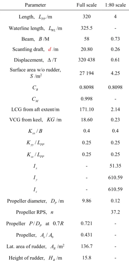
The MOERI KVLCC2 tanker hull and propeller is a benchmark test case for hydrodynamic applicatio- ns. In the CFD work, simulations have been carried out with the vessel at 1:80 scale, while the MMG model simulation uses full scale. The Table 1 shows the general parameters for the vessel at full scale and 1:80 scale[6]_.

Table 1 KVLCC2 general parameters

Parameter Full scale 1:80 scale

Length, L_PP/m 320 4

Waterline length, LWL/m 325.5 -

Beam, B/M 58 0.73

Scantling draft, d/m 20.80 0.26 Displacement, /T 320 438 0.61 Surface area w/o rudder,

S/m2 27 194 4.25

B

C 0.8098 0.8098

M

C 0.998 -

LCG from aft extent/m 171.10 2.14 VCG from keel, KG/m 18.60 0.23

/ xx

K B 0.4 0.4

/ yy PP

K L 0.25 0.25

/ zz PP

K L 0.25 0.25

x

I - 51.35

y

I - 610.59

z

I - 610.59

Propeller diameter, DP/m 9.86 0.12

Propeller RPS, n 37.2

Propeller P D/ P at 0.7R 0.721 - Propeller, A Ae/ 0 0.431 - Lat. area of rudder, AR/m2 136.7 - Height of rudder, H_R/m 15.8 -

Fig.1 Coordinate system

2. Mathematical model

The vessel can be considered as a rigid body. Assuming that the hydrodynamic forces and moments acting on the vessel are quasi-steadily and the lateral velocities are small compared to the forward speed which is not fast enough to take the wave making effect into account and the metacentric height of the vessel is sufficiently large to neglect the roll effect on the manoeuvring motions, the 3 degrees of freedom motion equations are presented as follows with respect to the body fixed coordinates system fixed at mid-ship position as shown in Fig.1.

2

( +m m u_x)&( +m m vr_y) (mx_GY r_r&) =X (1a)

( +m m v_y) + ( +& m m ur_x) + (mx_GY r Y_r&) =& (1b)

(I_zz+J r_zz) + (& mx_GN v ur_v&)( +& ) =N (1c)

Here terms on the right hand side are the external force components and yaw moment. And they can be further divided into three parts based on the MMG modular concept with the subscripts H, P, R to represent the forces and moments acting on the hull, the propeller and the rudder respectively in Eq.(2).

= _H + _P+ _R

X X X X (2a)

= _H+ _P+ _R

Y Y Y Y (2b)

= _H + _P+ _R

N N N N (2c)

The definitions of other nomenclature and symbols in Eq.(1) can be referred to any literature describing a standard MMG modelling procedure. In order to give an accurate prediction of ship manoeuvring motions, the key steps are to evaluate the above stated forces and moments correctly by proper models.

2.1 Hull forces and moments

shed by Kijima, hydrodynamic forces and moments acting on the hull can be expressed as follows[3]_:

2 2

= ( ) + + +

H vv vr rr

X X u X v X vr X r (3a)

2 2

= + + + + +

H v r v v r r vvr vrr

Y Y v Y r Y v v Y r r Y v r Y vr

(3b)

2 2

= + + + + +

H v r v v r r vvr vrr

N N v N r N v v N r r N v r N vr

(3c)

Here all the hydrodynamic derivatives on manoeu- vring, X_vv, X_vr, Xrr; Yv, Yr, Yv v, Yr r, Yvvr ,

vrr

Y ; Nv, Nr, Nv v, Nr r, Nvvr, Nvrr, which are

minimally influenced by scale effects can be derived from model tests, regression formulae or CFD simula- tion results directly. X u( ), representing the longitu- dinal resistance on the ship, can be obtained by refe- rring to several resistance charts, regression formulae, model tests or CFD calculation as well.

2.2 Propeller forces

The forces due to the propeller can be expressed as follows:

2 4

0

= (1 ) ( )

P p P T P

X t n D K J (4a)

= 0

P

Y , N_P= 0 (4b)

Here  is the density of water and tp0 is the thrust

deduction factor when the ship is advancing in a strai- ght line, which can be assumed to be constant during the manoeuvring motions for simplicity. The lateral force component and moment here are neglected due to their relatively small quantities and are included in the hull force part influenced by the propeller in MMG concept. The thrust coefficient KT can be

derived by 2nd order polynomial fitting as follows according to the open water characteristic test results

2

0 1 2

( ) = + +

T P P P

K J a a J a J (5)

The advanced ratio JP is defined as follows

(1 ) = P P P u J nD   (6)

where n, DP are the revolution speed and diameter

of the propeller respectively. The wake coefficient P

changes during the manoeuvring motions in general

and can be evaluated as

2 0

= exp( 4 )

P P P

    (7)

where P0 is the wake coefficient when ship advan-

cing straightly, and P is the geometrical inflow

angle to the propeller which can be derived as follows

=

P x rP

    (8)

Here xP denotes the non-dimensional longitudinal

coordinate of the propeller position.

2.3 Rudder forces and moments

Effective rudder forces and moment can be ex- pressed as follows:

= (1 ) sin

R R N

X  t F  (9a)

= (1+ ) cos

R H N

Y  a F (9b)

= ( + ) cos

R R H H N

N  x a x F  (9c)

Here xR is the longitudinal coordinate of the rudder

with the value of 0.5L_pp, while tR, aH, xH are the

coefficients representing the interaction between the hull and rudder. The rudder normal force FN is expre-

ssed as follows

2

1

= sin

2

N R R R

F A U f_  (10)

where AR denotes the rudder area and f, denoting

the rudder lift gradient coefficient, can be estimated by Fujii’s formula[7] _{which is commonly applied as} follows

6.13 =

+ 2.25

f_ 

 (11)

Here,  denotes the aspect ratio of the rudder. The non-dimensional effective rudder inflow velocity U_R can be estimated by Yoshimura’s model[8] _as:

= (1 ) 1+ ( )

R R

U  CG s (12a)

2

[2 (2 ) ] ( ) = (1 ) p R D s G s H s   

 (12b)

cos (1 )

= 1 U P

s

nP

 

where R denotes the wake coefficient at the rudder

position. The parameter C is the correction factor with different values for port side and starboard side rudder directions, 1.065 and 0.935 respectively[9]_{, due} to the asymmetric propeller slip stream effect. H_R is the rudder height and P is the propeller pitch.  is an experimental constant to reflect the acceleration effect by the propeller.

Regarding the effective rudder inflow angle R,

it can be derived by the following equations:

0

=

R R R

R

U u

     (13a)

=

R l rR

    (13b)

where 0 denotes the rudder angle with zero normal

pressure on the rudder, R is the flow straightening

coefficient and R is the effective inflow angle to

rudder with lR treated as an experimental constant

and can be set as 2xR for simplicity.

3. Generation of manoeuvring derivatives using CFD

The approach of using CFD simulations, rather than experimental tests or regression formulae, to generate the hydrodynamic derivatives on manoeu- vring required by the mathematical models has been in development for several years. Dedicated bench- marking workshops have been carried out since 2008[10]_{, with the most recent being held in December} 2014. Several key papers have been published in rela- tion to the approach in general such as Refs.[11-13].

In this work, 1:80 model scale simulations of the KVLCC2 vessel have been carried out using the commercial CFD software package StarCCM+, deve- loped by CD-Adapco. In order to obtain the linear manoeuvring derivatives, Planar Motion Mechanism (PMM) test simulations have been carried out and validated using experimental results. Oblique towing tests were also carried out in order to further validate the achieved results.

3.1 Simulation approach and set-up

In order to match the experimental results with which the CFD results were being validated, the un- appended hull without the propeller was simulated. An unsteady RANS approach was applied for all simulations. The CFD simulations were carried out in deep and calm water conditions to reduce complexity and enable faster generation of the required derivati- ves. The free surface was simulated using a volume of fluid approach where its location is tracked based on

the volume of air and water within the cells along the free surface. The Realizable Two-Layer k- turbule- nce model was applied throughout.

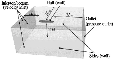
The hull was enclosed in a large rectangular computational domain with boundary conditions as shown in the Fig.2.

Fig.2 Domain and boundary conditions for KVLCC2 PMM test simulations

The automatic meshing tool within StarCCM+ was used, with additional areas of refinement added at the free surface. The resulting mesh consisted of app- roximately 7106 _{cells. A time-step size of 0.01 s was} applied.

Table 2 PMM test motion parameters

Pure sway Pure yaw Forward speed of

carriage, c

U /ms‒1

0.33156 (corresponds to

6 knots at full scale) 0.33156

Amplitude of

motion, a/m 0.3 0.1

Sway oscillation

frequency/s‒1 0.07 0.04

3.2 Planar motion mechanism (PMM) test simulations Two types of PMM tests were carried out at present, namely pure sway and pure yaw. In both cases, as in experimental tests, the vessel travels along a sinusoidal path with the forward moving carriage. In the pure sway simulations the heading angle of the vessel does not change, whilst for the pure yaw simu- lations, the heading of the vessel changes constantly to follow the path. For these simulations, the vessel was constrained in all 6 degrees of freedom. The parame- ters of the motion are outlined in the Table 2. It should be noted that the parameters were selected such that the heading angle of the vessel would be less than

o

10 due to the linear assumption for calculations of the linear derivatives. The parameters for the pure yaw simulations were also set to fulfill the requirement as

0

cos

tan = = = cos

c c

v a t

t

U U

 

Table 3 Comparison of manoeuvring derivatives

MMG regression MOERI EFD Simulation PMM Simulation oblique towing

v

Y −0.020892 −0.016190 −0.022392418 −0.0256669

v

Y& −0.014577 −0.015104 0.014176196 -

v

N −0.008606 −0.008754 0.014127218 −0.0076519

v

N& −0.001129 −0.000785 0.006413009 -

r

Y 0.005550 0.004720 −0.00704479 -

r

Y_& −0.001271 −0.001428 −0.00477182 -

r

N −0.003194 −0.003115 −0.02156711 -

r

N& −0.000729 −0.000800 −0.02299313 -

The time histories of the force in the y-direction and the moment about the z-axis acting on the vessel, in relation to a body-fixed coordinate system with the

-x axis aligned with the centreline of the vessel and centred at midships, were recorded. Then 8 linear manoeuvring derivatives required by the hull forces and moments evaluation module could be obtained by certain data processing procedure.

3.3 Oblique towing tests

Oblique towing tests of the vessel were carried out for drift angles of _6o_{, 4}o_{, 2}o_{, +2 ,}o ₊₄o _and

o

+6 . The resulting side force and moment acting on the vessel were then plotted against the lateral velocity, with the slope of the curves at the origin giving Y_v and Nv which believed to be more accurate and stable

than the ones obtained by the above mentioned PMM tests.

3.4 Generated results

The table below compares the values of the linear derivatives from the above mentioned tests by CFD, with those generated using regression formulae and from experimental data acquired at MOERI[10]_{. As} shown in the Table 3, whilst most of the velocity derivatives are reasonably close, the others do not show good agreement.

It was noted that the predictions arising from the CFD approach are very sensitive to a number of facto- rs, chiefly the selected motion parameters, but also the details of the mesh, meaning that without validation results, it would initially be very difficult to know if the results were reliable. For this reason, further deve- lopment and testing of the CFD approach is required. It is not at present clear why the derivatives arising from the pure yaw simulations are so unsatisfactory.

4. Results and discussion

4.1 Deep water case

As determined from the SIMMAN Website[6]_{, the} approach speed of the full scale KVLCC2 is taken as 15.5 knots in deep water corresponding to Froude number Fr= 0.142, and the rudder rate is assumed to be _{2.34 / s . The propeller rpm is assumed to be con-} o

stant during simulations.

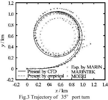
Fig.3 Trajectory of ₃₅o _{port turn}

Due to lack of suitable derivatives, only the first three velocity derivatives, generated from CFD simu- lations by pure sway tests as listed in Table 3, have been selected to be substituted into the mathematical model in place of the original regression based ones, while all the other derivatives are kept at their default empirical values. Figure 3 shows the trajectory of a standard ₃₅o _{rudder angle port turning motion by the}

regression formulae for all derivatives is also prese- nted. A detailed comparison of the characteristic para- meters of the turning motion between the measureme- nts and two simulations carried out by present pro- gram is given in Table 4. Generally speaking, both simulations have yielded good agreement with the measurements and even better than the simulations by other organizations as shown in Fig.3. On the other hand, the improvement of the results by substituting with the linear derivatives obtained from the PMM tests by CFD simulations seems insignificant since the nonlinear derivatives have not been generated by CFD calculations yet as which would significantly affect the accuracy of the results for large angle turning motions.

Table 4 Comparisons of turning characteristic parameters Present

CFD

Present empirical

MARIN

Advance 3.04L 2.9184L 2.98L

Transfer 1.4138L 1.3856L 1.266L

Turning radius 1.2821L 1.2211L 1.228L

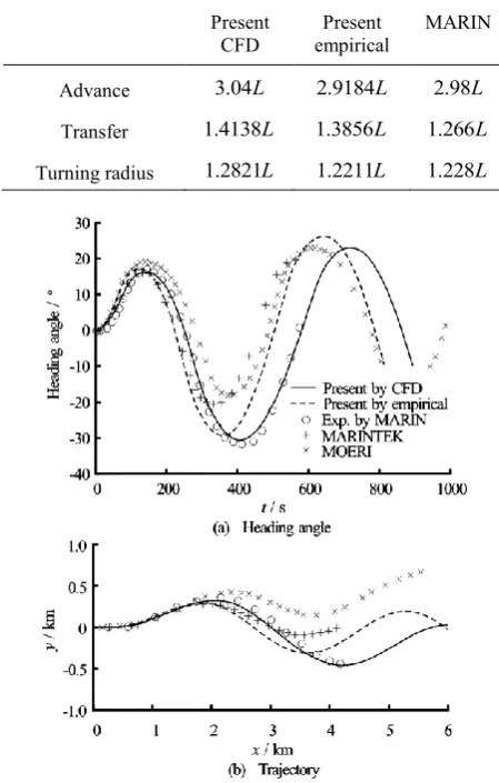
Fig.4 Time history of heading angle and trajectory of _{10 /10}o o Zig-Zag motion

Figure 4(a) shows the time history of the ship’s heading angle during a_{10 /10}o o _{Zig-Zag motion. And}

Fig.4(b) is the trajectory of the Zig-Zag motion. Like- wise, the measurements from MARIN tank, the simu- lations by MARINTEK and MOERI[10]_{, and the simu-}

lation by present program using the original regression based derivatives are again included for comparison. It can be found that the agreement between the measu- rements and both of the simulation results is good and better than the results by other organizations. More- over, remarkable improvements can be observed, according to the figures and the characteristic parame- ters of the motion listed in Table 5, by substituting the linear derivatives generated from CFD simulations when the vessel experiences small amplitude yaw motions which can be considered as linear problems.

Table 5 Comparisons of Zig-Zag characteristic parameters Present

CFD empirical Present MARIN 1st overshoot/o _{6.42 7.2 7.9} 2nd overshoot/o _{20.5 19.3 21.6}

Initial turning 1.92L 1.61L 1.94L

Fig.5 Trajectories of turning motion when heading angle up to o

40

4.2 Shallow water case

Simulation results for the shallow water condi- tion are in progress waiting for the manoeuvring deri- vatives from CFD calculations. Temporarily, the values of the derivatives from existing publication[4] obtained by model tests or CFD approach were used in the simulations based on a modified MMG model with the hull forces and moment evaluated by a 3rd order polynomial expression as follows:

2 2 4

= ( ) + + + +

H vv vr rr vvvv

X X u X v X vr X r X v (15a)

3 3 2 2

= + + + + +

H v r vvv rrr vvr vrr

3 3 2 2

= + + + + +

H v r vvv rrr vvr vrr

N N v N r N v N r N v r N vr

(15c)

The approach speed of the full scale KVLCC2 is set as 7 knots in shallow water simulations. Other initial conditions are the same as those in deep water.

Validations were carried out by comparing our results with the free running model tests conducted by KRISO[14] _{recently. 35}o _{turning manoeuvers were}

firstly executed until the heading angle of the ship reaches _{40 . The trajectories of the motions are illu-} o

strated in Fig.5 and the mean values of the characteri- stic parameters are listed in Table 6. Although oppo- site asymmetry of turning port and starboard side due to the propeller slip stream can be observed in the figure between the present simulations and the model tests, deviations of the mean values are small at the water depth of / =1.5h d . Besides, the tendency of longer distances with the decreasing water depth is captured which indicates that the shallow water effects would make the ship’s turning ability poorer. This is because the damping moment acting on the ship would increase when the ship turns in shallow water, which leads to lower yaw rates and smaller drift angles. Moreover, the speed loss would decrease due to smaller drift angles.

Table 6 Mean values of characteristic parameters when heading angle reaches ₄₀o

/

h d 1.5 1.2

Exp. Present Exp. Present

Mean X 1.69L 1.71L 2L 2.15L

Mean Y 0.29L 0.32L 0.39L 0.52L

Mean time/s 157 161 184 209

Then, _{20 / 5}o o _{Zig-Zag motions in shallow}

water were carried out with the time histories of the rudder and heading angles shown in Figs.6-9.

Fig.6 Time histories of rudder and heading angles during _{20 /}o o

5 Zig-Zag motions at h d/ =1.5

Fig.7 Time histories of rudder and heading angles during o o

20 /5

 Zig-Zag motions at h d/ =1.5

Fig.8 Time histories of rudder and heading angles during _{20 /}o o

5 Zig-Zag motions at h d/ =1.2

Fig.9 Time histories of rudder and heading angles during o o

20 /5

 Zig-Zag motions at h d/ =1.2

accurate coefficients obtained from CFD computatio- ns for the full scale ship. In addition, more free- running model tests should be conducted for compari- son.

Fig.10 Trajectories of _35o _{turn in deep and shallow water}

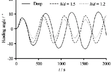
Fig.11 Time histories of heading angle of _{10 /5}o o _Zig-Zag motion in deep and shallow water

Once more, typical shallow water effects can be clearly seen in Fig.10 and Fig.11 by plotting the simu- lations in deep and shallow water together, which are the radius of the turning circle becoming larger with decreasing water depth according to the trajectories of

o

35

 turning motions and the improved course stabi- lity in shallow water according to the time histories of the heading angle of _{10 / 5}o o _{Zig-Zag motions respe-}

ctively.

5. Conclusion

In this paper, MMG model was applied for the standard manoeuving motion simulations performed on a full scale KVLCC2 ship. Regression formulae were firstly used to obtain the manoeuvring derivati- ves required by the model in the deep water simula- tions. Then CFD technique was introduced into the simulations in order to obtain the derivatives instead of empirical ones for higher accuracy. It can be confi- rmed that both sets of results derived by the present program are in good agreement with experimental measurements. Although it was also found that the

CFD results are very input-sensitive, there are promi- sing signs observed especially in the current predi- ction of the linearly dominated Zig-Zag manoeuver based on CFD results. Further study is required to improve the CFD approach. Furthermore, CFD results also need to be generated for the non-linear derivati- ves in order to have a full set of simulated rather than regression values. Finally, initial simulations in sha- llow water by a modified model with the data from existing publications are presented and compared with a set of model test results. The shallow water effects can be clearly captured from present simulations. These results can be considered as the benchmarks for further shallow water case studies based on CFD calculations in the near future.

Acknowledgements

This work is carried out within the scope of the ongoing collaborative EU Funded FP7 Framework Project SHOPERA (Energy Efficient Safe Ship Ope- ration) (Grant No. 605221 under the theme SST.2013.4-1). Results were obtained using the EPSRC funded ARCHIE-West High Performance Computer (www.archie-west.ac.uk). EPSRC (Grant No. EP/K000586/1).

References

[1] The Manoeuvring Committee. Final report and recommen- dations to the 25th ITTC[C]. 25thInternational Towing Tank Conference. Fukuoka, Japan, 2008, 1: 143-208. [2] OGAWA A., KOYAMA T. and KIJIMA K. MMG report-

I, on the mathematical model of ship manoeuvring[R]. Japan: The Bulletin of Society of Nval Architects of Japan, 1977, 575: 22-28.

[3] AOKI I., KIJIMA K. and FURUKAWA Y. et al. On the prediction method for maneuverability of a full scale ship[J]. Journal of the Japan Society of Naval Archite- cts and Ocean Engineers, 2006, 3: 157-165.

[4] YASUKAWA H., SANO M. Maneuvering prediction of a KVLCC2 model in shallow water by a combination of EFD and CFD[C]. 2nd Workshop on Verification and Validation of Ship Manoeuvring Simulation Methods. Kongens Lyngby, Denmark, 2014.

[5] YASUKAWA H., YOSHIMURA Y. Introduction of MMG standard method for ship maneuvering predictions[J]. Journal of Marine and Science Technology, 2015, 20(1): 37-52.

[6] SIMMAN Website.

http://simman2014.dk/ship-data/moeri-kvlcc2-tanker/geo-metry-and-conditions-moeri-kvlcc2-tanker/[OL]. 2014.

[7] FUJII H., TUDA T. Experimental research on rudder

performance[J]. Journal of the Society of Naval Archite- cts of Japan, 1961, 110: 31-42.

[9] HIRANO M. On calculation method of ship maneuvering motion at initial design phase[J]. Journal of the Society of Naval Architects of Japan, 1980, 147: 144-153. [10] The SIMMAN2008 Committee. Comparison of results for

free manoeuvre simulations[C]. Proceedings of SIMMAN 2008. 1st Workshop on Verification and Validation of Ship Manoeuvring Simulation Methods. Copenhagen, Denmark, 2008.

[11] SIMONSEN C. D., OTZEN J. F. and KLIMT C. et al. Maneuvering predictions in the early design phase using CFD generated PMM data[C]. 29th Symposium on Naval Hydrodynamics. Gothenburg, Sweden, 2012, 26- 31.

[12] STERN F., AGDRUP K. and KIM S. Y. et al. Experience from SIMMAN 2008The first workshop on verification and validation of ship Maneuvering simulation methods[J]. Journal of Ship Research, 2011, 55(2): 135-147. [13] ZOU Lu, LARSSON Lars and Orych Michal. Verification

and validation of CFD predictions for a manoeuvring tanker[J]. Journal of Hydrodynamics, 2010, 22(5Suppl.): 438-445.