Incremental dataset definition for large scale musicological research

City, University of London Institutional Repository

Citation

:

Wolff, D., Tidhar, D., Benetos, E., Dumon, E., Cherla, S. and Weyde, T. (2014).

Incremental dataset definition for large scale musicological research. In: Page, K. and Fields,

B. (Eds.), DLfM '14 Proceedings of the 1st International Workshop on Digital Libraries for

Musicology. (pp. 1-8). New York: ACM. ISBN 978-1-4503-3002-2

This is the accepted version of the paper.

This version of the publication may differ from the final published

version.

Permanent repository link:

http://openaccess.city.ac.uk/4076/

Link to published version

:

Copyright and reuse:

City Research Online aims to make research

outputs of City, University of London available to a wider audience.

Copyright and Moral Rights remain with the author(s) and/or copyright

holders. URLs from City Research Online may be freely distributed and

linked to.

City Research Online:

http://openaccess.city.ac.uk/

publications@city.ac.uk

Incremental Dataset Definition for Large Scale

Musicological Research

Daniel Wolff

daniel.wolff.1@city.ac.uk

Dan Tidhar

∗

dan.tidhar.1@city.ac.uk

emmanouil.benetos.1@city.ac.uk

Emmanouil Benetos

Edouard Dumon

edouard.dumon

@ensta-paristech.fr

Srikanth Cherla

srikanth.cherla.1@city.ac.uk

Research Group Dept. of Computer Science

City University London

Tillman Weyde

t.e.weyde@city.ac.uk

ABSTRACT

Conducting experiments on large scale musical datasets of-ten requires the definition of a dataset as a first step in the analysis process. This is a classification task, but metadata providing the relevant information is not always available or reliable and manual annotation can be prohibitively ex-pensive. In this study we aim to automate the annotation process using a machine learning approach for classification. We evaluate the effectiveness and the trade-off between accu-racy and required number of annotated samples. We present an interactive incremental method based on active learn-ing with uncertainty sampllearn-ing. The music is represented by features extracted from audio and textual metadata and we evaluate logistic regression, support vector machines and Bayesian classification. Labelled training examples can be iteratively produced with a web-based interface, selecting the samples with lowest classification confidence in each it-eration.

We apply our method to address the problem of instrumen-tation identification, a particular case of dataset definition, which is a critical first step in a variety of experiments and potentially also plays a significant role in the curation of digital audio collections. We have used the CHARM data-set to evaluate the effectiveness of our method and focused on a particular case of instrumentation recognition, namely on the detection ofpiano solo pieces. We found that uncer-tainty sampling led to quick improvement of the classifica-tion, which converged after ca. 100 samples to values above 98%. In our test the textual metadata yield better results

∗_{Dan Tidhar is also a member of the Department of Music}

at City University London.

†_{Edouard Dumon is also a member of ENSTA Paristech.}

than our audio features and results depend on the learning methods. The results show that effective training of a clas-sifier is possible with our method which greatly reduces the effort of labelling where a residual error rate is acceptable.

1.

INTRODUCTION

Digital libraries are growing quickly to sizes that render many research tasks too time consuming and costly when performed manually. Although standard library classifica-tion should include relevant classificaclassifica-tion data, the situa-tion in practice is that metadata is heterogeneous. It often comes from different sources, has been encoded by different standards and is of unknown quality and reliability. This situation is similar to other fields, such as health, geography and marketing, where the concepts and methods associated with the keywordBig Data have recently gained attention in many areas of research and applications. In order to ef-ficiently annotate and index digital collections of music, the statistical and machine learning techniques that enable au-tomation need to become part of the research method in digital musicology.

We are working on the adaptation of Big Data to musicology in the current Digital Music Lab1 _{project. As part of this}

project we apply automatic classification methods to define datasets for music research. Even answers to simple ques-tions, like the instrumentation of a piece, are not straight-forward to extract from existing metadata. With datasets that reach millions of audio, video and symbolic informa-tion items, manual labelling takes too long and is too costly. Therefore automatic classification is needed to reduce the human labelling effort and make large scale music research possible.

But even with automatic classifiers, a certain amount of training data is usually needed for supervised training. In this paper, we present an application of uncertainty sam-pling and active leaning in an effort to minimise the amount of training data needed for building high-performance clas-sifiers. We furthermore employ unsuperwised training in conjunction with Restricted Boltzmann Machines in an

ef-1

fort to further improve the classification performance using the remaining data yet to be labelled.

2.

RELATED WORK

Underwood et al. [19] present a principal example of the ap-plication of automatic classification algorithms to big datasets: They classify fiction literature from the period 1750-1850 by “point of view” into first person versus third person, with high accuracy on a pre-annotated set of 288 items, and ap-ply their method for further analysis on a dataset of over 30,000 titles.

The task of instrument identification is not new to the disci-pline of Music Information Retrieval (MIR). Earlier work, such as Ch´etry [5] focuses on identifying instruments in isolated instrument recordings, whereas later work such as Giannoulis and Klapuri [10] handles mixed instruments in polyphonic audio.

It should be noted that the problem of instrument iden-tification is indeed related but is certainly not identical to the problem at hand:instrumentationidentification is moti-vated by our need to characterise recordings according to the

entire setof instruments taking part in a track (in the con-text of classical music this can be thought of as one possible way of sub-genre classification). With very few exceptions, this variant of the problem has not so far been approached in the literature. One such exception is provided by Schedl and Widmer [16], who use web-mining and a purely text-based approach to obtain information about band members and in-strumentation for Rock tracks. Barbedo and Tzanetakis [2] apply audio-based instrument recognition to polyphonic au-dio by extracting segments in which individual instruments appear in isolation. Brown [4] apply MFFC-based classifica-tion to detect specific instruments (clarinet and saxophone) and carefully select their test set to contain these instru-ments in isolation. Itoyama et al. [14] combine source sepa-ration methods with Bayesian instrument classification and successfully apply their instrument identification techniques to mixtures of 2-3 instruments. All the above citations make valuable contributions to the field, yet do not provide a fea-sible direct solution to our particular problem due to per-formance limitations and due to the crucial difference in the problem formulation as explained above.

3.

THE CHARM DATASET

In this study we use a dataset published by the AHRC Re-search Centre for the History and Analysis of Recorded Mu-sic (CHARM) (2004-2009). It contains digitised versions of nearly 5000 copyright-free historical recordings, dated (1902-1962) as well as metadata describing both the provenance of the recordings and the digitisation process.

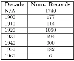
The richness of annotations in the CHARM dataset as well as its size render it a good subject of musicological analysis using computational methods. Table 2 shows the distribu-tion of included records over time, with the most included items being recorded between 1920 and 1950. The com-posers with the most recorded pieces in the dataset are Schu-bert, Mozart, Bach, Beethoven, Brahms, Wagner, Haydn and Chopin.

3.1

Ground Truth for Piano Solo

For our first classification experiments and to bootstrap our sampling process we annotated a sample of 591 recordings in the CHARM dataset regarding to their instrumentation by listening into the acoustic content of the pieces as well as taking into account the existing metadata. A histogram of those annotations is given in Table 1.

Instrumentation Count

piano solo 133 orchestra 123 vocal + orchestra 64 chamber 42

choir 40

vocal + piano 40 violin + piano 37 string quartet 25 vocal + organ 20

organ 13

piano + orchestra 9 piano duet 7

violin 7

piano quartet 6 harpsichord 5

vocal 5

cello + piano 4 vocal + harp 3 organ + orchestra 2 violin + harpsichord 2

banjo 1

brass 1

oboe + piano 1 viola + piano 1 Total 591

Table 1: Histogram of our expert annotations on the CHARM data subset.

In the present paper we focus on whether pieces are an-notated as piano solo or otherwise. The piano solo cate-gory marks music that contains only piano as an instrument through the whole recording. Out of all annotated pieces, 133 fall into this category, and 458 recordings were anno-tated as the mutually exclusive categorynot solo piano.

Decade Num. Records

N/A 1740 1900 177 1910 114 1920 1060 1930 694 1940 900 1950 182 1960 6

Artist Composer Notes Title

519 246 335 1074

Table 3: Number of unique terms in each metadata field.

4.

FEATURE EXTRACTION

For representing the CHARM dataset to the classifier, we extracted a set of features representing the different sources of information. In order to compare their effectiveness, we extracted features from the metadata and audio, and later test their individual and combined effect on classification performance in Section 6.2.

4.1

Metadata

One of the outputs of CHARM is a spreadsheet contain-ing manually created metadata for the entire dataset. The spreadsheet associates with each file name several metadata fields, some related to the recording itself (such as title, artist, composer) and some relating to the digitisation pro-cess (including stylus weight and speed). Additionally, there is a field titled ”Notes” which sometimes includes some in-formation about instrumentation (e.g. in some piano solo recordings, but certainly not all, it contains the string ”Pi-anoforte solo”), it is often empty, and sometimes also in-cludes other notes inserted by the CHARM team.

Since the different fields potentially have different contribu-tions to our classification task, and in order to avoid ex-tremely sparse representations, we applied a standard bag-of-words feature extraction, separately to each metadata field.

We transferred the contents of the metadata spreadsheet to a MySQL database, and extracted the bag of words frequency vectors in the following manner: For each of the relevant fields (Title, Artist, Composer, Notes), we created a separate list of words containing all the words that appear in that field across the entire database. Table 3 contains the number of unique terms found for each of those fields.

For each file, we then collected the term frequencies in four separate vectors (one for each field), with a dimensional-ity corresponding to the respective number of unique terms. The vectors were then concatenated to yield the metadata featuresx∈R2174.

4.2

Instrumentation Audio Features

In order to estimate instrumentation directly from poly-phonic audio, we employed the efficient automatic music transcription method of Benetos et al. [3]. The transcrip-tion system is based on probabilistic latent component anal-ysis, which is a spectrogram factorisation technique that is able to produce a pitch activation matrix (useful for multi-pitch detection) but also an instrument contribution matrix (useful for instrument assignment experiments).

In specific, the model takes as input a normalised log-frequency spectrogramVω,tand approximates it as a bivariate

proba-bility distributionP(ω, t), which is in turn decomposed as:

P(ω, t) =P(t)X

p,f,s

P(ω|s, p, f)Pt(f|p)Pt(s|p)Pt(p) (1)

s

P

(

s

)

0 2 4 6 8 10 12 14

0 0.05 0.1 0.15 0.2 0.25

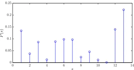
Figure 1: Extracted instrumentation features for an orchestral recording from the CHARM database. Index s corresponds to (from left to right): piano1, piano2, piano3, cello, clarinet, flute, guitar, harpsi-chord, oboe, violin, tenor sax, bassoon, and horn.

where P(ω|s, p, f) are pre-extracted spectral templates for pitchpand instruments, which are shifted across log-frequency according to parameter f. P(t) is the spectrogram energy (known quantity),Pt(f|p) is the time-varying log-frequency

shifting for pitch p,Pt(s|p) is the instrument contribution,

and Pt(p) is the pitch activation. All unknown parameters

can be estimated iteratively using the Expectation-Maximi-sation algorithm (15-20 iterations are required for conver-gence).

In order to extract instrumentation features, the instrument contribution Pt(s|p) is used. We first create a joint

prob-ability distribution of instruments, pitches and time using estimated parameters:

P(s, p, t) =Pt(s|p)Pt(p)P(t) (2)

Subsequently, we marginalise the joint distribution in or-der to compute a probability of each instrument across all pitches, for the complete duration of each recording:

P(s) =X

p,t

P(s, p, t) (3)

For the specific experiments, the transcription system used a dictionary of pre-extracted templates for bassoon, cello, clarinet, flute, guitar, harpsichord, horn, oboe, piano, tenor sax, and violin. Templates were extracted using isolated note samples from the RWC database of Goto et al. [11], as well as the MAPS database of Emiya et al. [8]. The length ofswas 13, covering 3 piano templates as well as one template for each other instrument. As an example, Figure 1 shows the instrumentation featuresx∈R13extracted for an

orchestral music recording.

4.3

Combined Features

It has been shown that the combination of different feature types can improve performance of classification methods. We therefore generate combined features by concatenating all metadata and audio features, resulting in feature vectors

1

. . .

. . .

W c

b

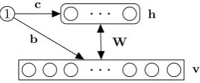
Figure 2: A simple Restricted Boltzmann Machine with four visible, two hidden, and no bias units.

4.4

RBM Feature Transformation

The large dimensionality and sparsity of the features de-scribed above motivates the use of a feature-transform that might potentially reduce the dimensionality and increase the efficiency of the feature representation. Restricted Boltz-mann Machines (RBMs) can be used for learning such a transformation that furthermore increases the complexity of functions which can be represented by linear models such as Support Vector Machines (SVMs) (see Section 5.3). The RBM is an undirected, bipartite graphical model con-sisting of a set ofr units in its visible layer v and a set of

qunits in itshidden layer h(Figure 2). The two layers are fully inter-connected by a weight matrixWr×qand there

ex-ist no connections between any two hidden units, or any two visible units. Additionally, the units of each layer are con-nected to a bias unit whose value is always 1. The weights of connections between visible units and the bias unit are contained in thevisible bias vectorbr×1. Likewise, for the

hidden units there is thehidden biasvectorcq×1. The RBM

is fully characterised by the parametersW,bandc. In its original form, the RBM has binary, logistic units in both layers. The activation probabilities of the units in the hidden layer given the visible layer (and vice versa) are de-termined by the logistic sigmoid function asp(hj= 1|v) =

σ(cj+Wj·v), andp(vi= 1|h) =σ(bi+Wi0·h) respectively.

Due to the RBM’s bipartite structure, the activation proba-bilities of the nodes within one of the layers are independent, if the activation of the other layer is given, i.e.

p(h|v) =

q Y

j=1

p(hj|v) (4)

p(v|h) =

r Y

i=1

p(vi|h). (5)

This property of the RBM makes it suitable for learning a non-linear transformation of an input feature space [6]. This is typically carried out in two steps: (1) unsupervised pre-training, and (2) supervised fine-tuning of the model[13]. Pre-training is done using the Contrastive Divergence algo-rithm [12], and fine-tuning using backpropagation [15]. Transformed features obtained after each of these steps, when used with the original features, have been found to improve the performance on a classification/prediction task [13]. In the present paper, we transform the audio features with an RBM trained only in an unsupervised manner.

5.

ACTIVE LEARNING WITH

INCREMEN-TAL TRAINING SETS

We formulate the task of detecting whether a pieces instru-mentation corresponds topiano soloor not as a binary clas-sification task:

y= classify(x) (6) Here, y ∈ {0,1}2 _{is the binary representation of the class}

(1 representing piano solo and 0 any other instrumentation) andx∈Rcorresponds to the feature vector describing the

record in question.

In this paper we explore how automatic classifiers can be trained to high performance using a minimal amount of data training data. With the perspective of building interactive access and research tools for large music collections, we fol-low the paradigms of incremental and interactive data col-lection. The data collection is controlled by active learning, i.e. the learning systems determines which data next to re-quest labels for from the human annotator [1, 17].

In order to facilitate incremental data collection, we imple-mented a web interface based on Wolff et al. [20]. The gamified interface provides annotators with an additional incentive to contribute, while allowing annotations to be dis-tributed in time and in space. The system’s training data can be updated either after each submission, or alternatively, submissions can be accumulated and processed as batch if the user base grows and heavier traffic is expected.

Figure 3: A screenshot of the gamified web interface for incremental annotation.

Depending on the algorithm, learning from added training data can be accomplished by retraining models with the ex-tended training sets or by online learning, which allows mod-els to adapt to new training data by modifying some of the learnt parameters. In the experiments below, we simulate active learning by incrementally sampling from the training data and retraining the models.

5.1

Uncertainty Sampling

In our experiments we select new training samples using a confidence measure. The goal is to query the human an-notator about samples that the automatic classifier is most

2

uncertain about. To this end we define confidence measures which describe the confidence of a model for classifying a specific sample.

The definition of this measure and possible alternatives de-pend on the classifier type. For probabilistic classifiers, we measure uncertainty using the classifier’s prediction proba-bility of both classes. Letx be the feature vector, then we derive the confidence as the sum of the absolute values of the probability estimates:

confidence =|P(y= 1|x)−0.5|+|P(y= 0|x)−0.5| (7) For the SVM algorithm described in Section 5.3, where this estimate is not available, we use the distance of x to the hyperplanewwhich was learnt to separate the classes. We now describe the algorithms evaluated in our experi-ments. Our experiments are based on the implementations in the python frameworkscikit-learn3_.

5.2

Logistic Regression

A standard tool in classification, Logistic Regression (LREG) can be used to predict a binary target vector from a binary input. The conditional probability of an output given the input is defined by

Pw(y=±1|x) =

1

1 +e−yw|x. (8)

Here,wis a weight vector,xcorresponds to the input fea-tures of a record andyis the output classification.

In our experiments we use theliblinear4implementation as included in scikit-learn. We chose to use the L2-norm for penalising unmatched training data, a stopping criteria tol-erance of 10−8 and add a constant intercept to the model. We furthermore employ only weak regularisation using a reg-ularisation factor of C = 100000.0. For further details on the optimisation procedure see Yu et al. [21].

5.3

Support Vector Machines

A SVM [7] is a non-probabilistic binary linear classifier which constructs a hyperplane in a high- or infinite-dimensional space, which can be used for classification or regression. This mapping to a higher-dimensional space than the one in which features originally reside helps in achieving lin-ear separability which may not always be the case in the lower-dimensional space. Moreover, the mapping is designed to ensure that dot-products may be computed efficiently in terms of the variables in the original space, by defining them in terms of akernel function selected to suit the problem. The hyperplanes in the higher-dimensional space are defined as the set of points whose dot-product with a vector in that space is constant. And while there may be many hyper-planes which classify a given set of features correctly, the SVM chooses the one that represents the largest separa-tion, or margin, between two classes. This is known as the

maximum-margin hyperplane. The samples on the margin are known asSupport Vectors.

3_{http://scikit-learn.org} 4

http://www.csie.ntu.edu.tw/~cjlin/liblinear/

Given a training set of feature-label pairs (xi, yi) wherexi∈

Rn andy ∈ {1,−1}, the SVM requires the solution of the following optimisation problem:

min

w,b,ξ

1 2w

T w+C

l X

i=1

ξi (9)

subject to yi(wTφ(xi) +b)≥1−ξi,

ξi≥0,

where the function φ maps the training feature vectors xi

into the higher-dimensional space. C > 0 is the penalty parameter of the error term. K(xi,xj) ≡ φ(xi)Tφ(xj) is

the aforementioned kernel function.

While several different kernels of differing complexities are available, in the present work we employ a linear kernel which is defined asK(xi,xj) =xTixj. This linear SVM can

be solved efficiently by gradient methods such as coordinate descent [9].

We here compare the implementation based on liblinear, with parametersC= 105 _{as well as the stochastic gradient}

descent version directly implemented inscikit-learn, which we call Stochastic Gradient Descent (SVMGD).

5.4

Multinomial Naive Bayes

A Multinomial Naive Bayes (BAY) classifier is a probabilis-tic model. The conditional probability of a recordd belong-ing to classcis computed as

P(c|d)∝P(c) Y

1≤k≤n

P(xk|c) (10)

where n is the feature vector size and xk the k-th feature

element. We use a multinomial distribution with Laplacian smoothing as the event model P(f|c). The underlying as-sumption of Naive Bayes is that the features are indepen-dent, which is generally a simplification. Nevertheless, it has been been used successfully in text classification [22]. The probabilities can be updated incrementally, thus supporting online learning.

6.

EXPERIMENTS

For our experiments we used 4-fold cross-validation, which split the ground truth data into randomly selected sets of training data used for fitting the classifiers, and test sets for analysing their generalisation performance: The data were split into four subsets. Special characteristics of the meta-data such as artists were not considered when splitting the dataset. In each of four iterations, three subsets were used as training sets and the remaining one as test set. The param-eters concerning regularisation during training of the differ-ent classifiers as reported in Section 5 where determined in previous experiments on the CHARM dataset.

6.1

Overall Performance

classify the test data with less than 6% error rate given the full training set. In particular, the SVM-based and RBM approaches achieve less than 3% error, RBM providing the top performance in this comparison. The online-learning BAY algorithm shows the worst performance, which is in line with earlier experiments, and motivates future exper-iments on the parametrisation of online learning with un-certainty sampling. Given the high dimensionality of the combined features, the good performance of the algorithms is probably related to close relations of terms such as artists or further annotations in the metadata features to thepiano soloclassification. Regarding this property, CHARM is not exceptional and the good results should very well apply to other datasets.

In order to assess the effectiveness of uncertainty sampling as described in Section 5.1, we also analyse how fast the al-gorithms converge to their final performance when the train-ing set grows incrementally. The number of traintrain-ing samples needed is determined as the point where an algorithm’s per-formance does not exceed its perper-formance for the full train-ing set (final err) by more than 1%. Considertrain-ing that the measured standard deviation of the algorithms along the cross validation folds averages around 1%, we choose this heuristic as an indicator of the effectiveness of our approach of uncertainty sampling.

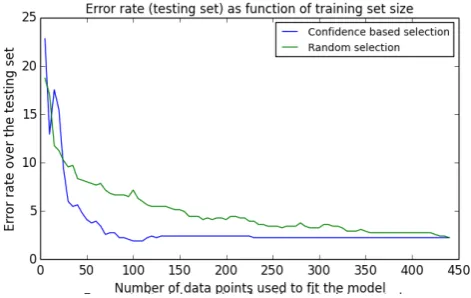
In Figure 4, the test set performance of SVM is plotted for uncertainty sampling (“Confidence-based selection”, blue curve) and Random selection (green curve) for adding train-ing data. While the blue curve reaches the final performance with only 85 training examples, the performance of random selection only converges to the same performance with all training examples.

As can be seen in the first column of Table 4, uncertainty sampling can achieve improved performance earlier – with less training data – for all classifiers. Random sampling does only reach its best performance with the full or considerably larger training sets. Table 4 also reports the classification er-ror difference at the number of training constraints sufficient for uncertainty sampling to approach its best performance within 1%. We call this a plateau. Except for the RBM approach, the random sampling performs worse than uncer-tainty sampling when this plateau is reached. The RBM features allow better results even when no uncertainty sam-pling is used.

Figure 5 shows the confidence of classifications on the test set for SVM. The blue curve corresponding to uncertainty samling reaches higher confidence on the unknown test set when compared to random sampling. While the training set confidence (not plotted here) is low due to the explicit selection of such data, we find that selecting this data is beneficial for faster learning and better generalisation.

6.2

Feature Type

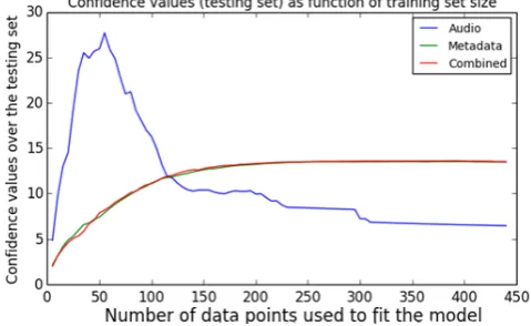
It has been shown that feature information also strongly in-fluences a classifier’s generalisation performance. We com-pared the performance of metadata, audio and combined features. Our experiments showed that metadata features performed well with or without the audio features. Audio features on the other hand only allowed for low performance

Figure 4: Test set performance of SVM. The bottom blue curve corresponds to uncertainty sampling, the top green curve measures random sampling.

Figure 5: Confidence of classifications on the test set for SVM. The bottom blue curve corresponds to uncertainty sampling, the top green curve measures random sampling.

with an error around 10% when used on their own, as is plotted for logistic regression in Figure 6. Still, uncertainty sampling outperforms random sampling on small training sets.

When examining the confidence values, again with logistic regression, for the different feature types as plotted in Fig-ure 7, we found that acoustic featFig-ures actually lost confi-dence on the test set after starting with high conficonfi-dence. This might be related to a misinterpretation of audio fea-tures relating to the labels that gathers high confidence and misleads the iterative optimisation. Still, the performance reported for acoustic features is similar to the human per-formance for classifying isolated instruments into 9 classes based only on listening as reported by Srinivasan et al. [18].

6.3

Batch Sizes

method first plateau err@plateau rand.err@plateau final err train err

LREG 55 3.06 8.67 3.23 0.0 SVM 85 2.210 6.63 2.21 0.0 SVMGD 140 2.38 5.10 2.38 0.0 LREG + RBM 325 2.04 3.40 2.04 0.0 BAY 55 5.10 5.78 5.95 0.68

Table 4: Overall classification performance of the tested algorithms in percentage of misclassifications. “first plateau” counts the training samples needed to reach the final performance within 1% in our uncertainty sampling approach. The performance of uncertainty (err@plateau) and random sampling (rand.err@plateau) for this point are reported. The rightmost columns list the test and training error for the full training set.

Figure 6: Performance of the audio features for ran-dom and uncertainty sampling. The performance is relatively low in both cases.

Figure 7: Comparison of feature types’ effects on the confidence of test set classifications. Audio features perform badly with large training sets.

Figure 8: Comparison of different increment sizes over growing training sets. Smaller increments show better performance with few training data.

especially with small numbers of training data. Small batch sizes gain higher performance and a batch size of 5 items added per training cycle seems optimal.

7.

CONCLUSION

7.1

Future Work

We are looking forward to applying this experiment in a real-time active learning experiment involving the gamified version of the data collection interface as presented above. The presented method can be directly applied to the anno-tation of (music) datasets with similar metadata.

Where metadata is lacking, more research is needed into audio features that provide more relevant information to the task of instrumentation recognition. For instance, rep-resentation of the audio features learned by the RBM can be further improved with the additional fine-tuning step as mentioned in Section 4.4.

The resulting interfaces and learning methods will be fur-thermore employed in the AHRC Digital Transformations project Digital Music Lab for annotating large scale music data in an interactive infrastructure for music research.

8.

ACKNOWLEDGEMENTS

This work is supported by the AHRC project “Digital Music Lab - Analysing Big Music Data”, grant no. AH/L01016X/1. Emmanouil Benetos is supported by a City University Lon-don Research Fellowship.

References

[1] Hybrid active learning for reducing the annotation ef-fort of operators in classification systems. Pattern Recognition, 45(2):884 – 896, 2012. ISSN 0031-3203. [2] J. G. A. Barbedo and G. Tzanetakis. Musical

in-strument classification using individual partials. IEEE Transactions on Audio, Speech, and Language Process-ing, 19(1):111–122, Jan. 2011.

[3] E. Benetos, S. Cherla, and T. Weyde. An efficient shift-invariant model for polyphonic music transcription. In

6th International Workshop on Machine Learning and Music, Prague, Czech Republic, Sept. 2013.

[4] J. C. Brown. Computer identification of musical in-struments using pattern recognition with cepstral coef-ficients as features.Journal of the Acoustical Society of America, 105(3):1933–1941, Mar. 1999.

[5] N. D. Ch´etry.Computer Models for Musical Instrument Identification. PhD thesis, Queen Mary, University of London, 2006.

[6] A. Coates, A. Y. Ng, and H. Lee. An analysis of single-layer networks in unsupervised feature learning. In

International Conference on Artificial Intelligence and Statistics, pages 215–223, 2011.

[7] C. Cortes and V. Vapnik. Support-vector networks.

Machine learning, 20(3):273–297, 1995.

[8] V. Emiya, R. Badeau, and B. David. Multipitch esti-mation of piano sounds using a new probabilistic spec-tral smoothness principle. IEEE Transactions on Au-dio, Speech, and Language Processing, 18(6):1643–1654, Aug. 2010.

[9] R.-E. Fan, K.-W. Chang, C.-J. Hsieh, X.-R. Wang, and C.-J. Lin. Liblinear: A library for large linear classifi-cation. The Journal of Machine Learning Research, 9: 1871–1874, 2008.

[10] D. Giannoulis and A. Klapuri. Musical instrument recognition in polyphonic audio using missing feature approach. IEEE Transactions on Audio, Speech, and Language Processing, 21(9):1805–1817, 2013.

[11] M. Goto, H. Hashiguchi, T. Nishimura, and R. Oka. RWC music database: music genre database and musi-cal instrument sound database. In International Sym-posium on Music Information Retrieval, Oct. 2003. [12] G. E. Hinton. Training products of experts by

minimiz-ing contrastive divergence. Neural computation, 14(8): 1771–1800, 2002.

[13] G. E. Hinton and R. R. Salakhutdinov. Reducing the dimensionality of data with neural networks. Science, 313(5786):504–507, 2006.

[14] K. Itoyama, M. Goto, K. Komatani, T. Ogata, and H. G. Okuno. Simultaneous processing of sound source separation and musical instrument identification using Bayesian spectral modeling. In IEEE International Conference on Acoustics, Speech and Signal Processing, pages 3816–3819, May 2011.

[15] D. E. Rumelhart, G. E. Hinton, and R. J. Williams. Learning representations by back-propagating errors.

Cognitive modeling, 1988.

[16] M. Schedl and G. Widmer. Automatically detecting members and instrumentation of music bands via web content mining. In N. Boujemaa, M. Detyniecki, and A. N¨urnberger, editors,Adaptive Multimedia Retrieval: Retrieval, User, and Semantics, volume 4918 ofLecture Notes in Computer Science, pages 122–133. Springer Berlin Heidelberg, 2008. ISBN 978-3-540-79859-0. doi: 10.1007/978-3-540-79860-6 10.

[17] B. Settles. Active learning literature survey. Technical report, University of Wisconsin–Madison, 2010. [18] A. Srinivasan, D. Sullivan, , and I. Fujinaga.

Recogni-tion of isolated instruments tones by conservatory stu-dents. InIn Proc. ICMPC, 2002.

[19] T. Underwood, M. Black, L. Auvil, and B. Capitanu. Mapping mutable genres in structurally complex vol-umes. In 2013 IEEE International Conference on Big Data, Santa Clara, CA, 10/2013 2013.

[20] D. Wolff, G. Bellec, A. Friberg, A. MacFarlane, and T. Weyde. Creating audio based experiments as social web games with the casimir framework. In Proc. of AES 53rd International Conference: Semantic Audio, Jan 2014.

[21] H.-F. Yu, F.-L. Huang, and C.-J. Lin. Dual co-ordinate descent methods for logistic regression and maximum entropy models. Mach. Learn., 85(1-2): 41–75, Oct. 2011. ISSN 0885-6125. doi: 10. 1007/s10994-010-5221-8. URL http://dx.doi.org/ 10.1007/s10994-010-5221-8.