J-SELF-ADJOINT BLOCK OPERATOR MATRICES
MATTHIAS LANGER AND MICHAEL STRAUSS
Abstract. We study the spectrum of unboundedJ-self-adjoint block opera-tor matrices. In particular, we prove enclosures for the spectrum, provide a sufficient condition for the spectrum being real and derive variational princi-ples for certain real eigenvalues even in the presence of non-real spectrum. The latter lead to lower and upper bounds and asymptotic estimates for eigenval-ues.
AMS Subject classification 2010: 47B50, 47A10; 47A56, 46C20, 49R05.
Keywords: J-self-adjoint operator, spectral enclosure, Schur complement, quadratic numerical range, Krein space, spectrum of positive type.
1. Introduction
Let H1 and H2 be Hilbert spaces and consider a block operator matrix acting in
the direct sumH:=H1⊕ H2, i.e. an operator of the form M0=
A B C D
,
where, e.g.Ais an operator inH1andBan operator fromH2toH1. Such operators play an important role in many spectral problems and their applications; see, e.g. the monograph [30] and the references cited therein. In recent years, many papers have studied and described spectral properties of such block operator matrices in terms of their entries A, B, C and D. In particular, spectral enclosures and variational principles for characterising eigenvalues, often in a gap in the essential spectrum, have received a great deal of attention; see, e.g. [1, 3, 4, 5, 9, 13, 15, 17, 19, 21, 24, 25, 26, 28, 29]. In many of these papers the case was studied when A and D are self-adjoint andC=B∗, in which caseM0 is a symmetric operator in
H, and often even essentially self-adjoint.
In the present paper we consider the situation when A and D are self-adjoint and C =−B∗. In this case the operator M0 is J-symmetric whereJ = I0−I0 ; this means thatJM0is a symmetric operator inH, or in other words, the operator
M0 is symmetric in the Krein space K:=H1⊕ H2 with indefinite inner product [x, y] := hJ x, yi, where h·,·i denotes the inner product in the Hilbert space H. Every bounded self-adjoint operator in a Krein space can be written as a block operator matrix with A, D self-adjoint and C = −B∗. However, this is not true in general for unbounded operators. Moreover, for given self-adjoint A, D and C = −B∗ it is not guaranteed that M0 has a closure that is self-adjoint in the
Krein space. Even if the latter is true, it is not clear whether this closure has non-empty resolvent set.
We consider two classes of unbounded block operator matrices: certain upper dominant matrices (where the operators in the top row, i.e. Aand B are stronger than those in the bottom row in the sense that the latter are relatively bounded with respect to the former) and certain diagonally dominant matrices (where the stronger operators are the diagonal operators A and D). In these situations the
operator M0 is closable, its closure M is J-self-adjoint, i.e. self-adjoint in the
Krein space, and it has non-empty resolvent set. Certain diagonally dominant J-self-adjoint block operator matrices, often with bounded B or some other extra assumptions, have been investigated, e.g. in [1, 3, 4, 15, 19, 20, 21, 29]. However, to our knowledge, upper dominant J-self-adjoint block operator matrices have been studied only in few papers; see [15, 28].
Since in both cases that we consider (upper and diagonally dominant case) the operator A is stronger in some sense thanC =−B∗, there exista∈R andb≥0 such thatkB∗xk2≤akxk2+bhAx, xifor allx∈dom(A). Using these constantsa, b
and the location of the spectra ofAandDwe prove enclosures for the spectrum of
M. In particular, the non-real spectrum is always contained in a compact set and hence the resolvent set is non-empty; see Theorem 4.13. We also give a sufficient condition for the spectrum of Mbeing real, namely condition (A) introduced in Definition 4.5. In the latter situation we can give an enclosure that consists of one interval (in a limiting case) or of two disjoint intervals (in the generic case). The main tool for proving these enclosures is the quadratic numerical rangeW2(M)⊂
C, which was introduced in [26] and whose closure contains the spectrum in many situations; see Definition 4.1 and Proposition 4.12.
The second set of results concerns the characterisation of certain eigenvalues with variational principles. Instead of the classical Rayleigh quotient we use either a functional that is connected with the quadratic numerical range (see Theorem 5.12) or a generalised Rayleigh functional that is associated with the Schur complement of the block operator matrix (see Theorem 5.6); the Schur complement is formally given by
S(z) =A−z+B(D−z)−1B∗
and is an operator function acting only in the first componentH1. With the help of these variational principles we also prove enclosures for eigenvalues ofMas well as asymptotic enclosures under the extra assumption thatAhas compact resolvent.
Further, we prove some results concerning the properties ofMconsidered as an operator in a Krein space. In particular, we prove that spectral points in a certain interval are of positive type, and therefore there exists a local spectral function for the operator M. If Ahas compact resolvent, thenM is definitisable. Finally, we discuss some examples with differential operators as entries to illustrate our results. Let us give a brief synopsis of the paper. In Section 2 we define the operator
Notation. For a linear operator T we denote its spectrum by σ(T) and its resolvent set byρ(T). In addition, we define theessential spectrum,point spectrum, discrete spectrum,approximate point spectrumand thenumerical range as follows:
σess(T) :=
z∈C:T−zis not Fredholm , σp(T) :=
z∈C: ker(T−z)6={0} ,
σdis(T) :=z∈σp(T) :T−z is Fredholm andzis isolated in σ(T) ,
σapp(T) :=
z∈C:∃xn∈dom(T),kxnk= 1,(T−z)xn →0 , W(T) :=hT x, xi:x∈dom(T),kxk= 1 .
The square root of a real number is defined such that √t ≥0 for t ∈ [0,∞) and Im√t >0 for t ∈(−∞,0). Moreover, we use the notation (t)+ := max{t,0} for
t∈R.
2. J-self-adjoint operator matrices
Throughout this paper letH1andH2 be Hilbert spaces with inner productsh·,·i; we also denote the inner product in H:=H1⊕ H2 byh·,·i. Moreover, let Abe a self-adjoint operator acting inH1which is bounded from below; letB be a densely defined and closable operator acting from H2 to H1; and letD be a self-adjoint operator acting in H2 which is bounded from above. Let a and d be the closed
quadratic forms associated with the operators AandD, respectively, and set α−:= minσ(A), δ+:= maxσ(D). (2.1)
We shall be concerned with the spectral properties of (the closure of) the block operator matrix
M0:=
A B
−B∗ D
:H1⊕ H2→ H1⊕ H2 (2.2) with dom(M0) = dom(A)∩dom(B∗)× dom(B)∩dom(D). We consider two classes of matrices, which are introduced in the following assumption.
Assumption 2.1. LetA,B,D andM0 be as above. We assume that one of the
following conditions is satisfied:
(I) dom(a)⊂dom(B∗), dom(B)⊂dom(D), dom(B) is a core forD; (II) dom(a)⊂dom(B∗), dom(d)⊂dom(B).
Under Assumption 2.1.(I) the block operator matrix M0is upper dominant in the sense that the operators in the second row are relatively bounded with respect to the operators in the first row; see [30, Definition 2.2.1]. If Assumption 2.1.(II) is satisfied, then M is diagonally dominant. As we shall see below, M0 is closed in case (II) and closable in case (I). In both cases, we denote the closure of M0 by
M.
The condition dom(a)⊂dom(B∗) (which is satisfied in both cases (I) and (II)) ensures the existence of constantsa∈Randb≥0 such that
kB∗xk2≤akxk2+ba[x] for all x∈dom(a). (2.3)
Clearly, one can choose a and b such that both are non-negative, but we allow a to be negative to have more flexibility in our estimates. Moreover, let b0 be the
relative bound, i.e. b0:= inf
However, for many theorems, in particular, in later sections, we fix one pair a, b such that (2.3) holds.
Remark 2.2. Relation (2.3) implies that, forx∈dom(a)\{0},
0≤kB
∗xk2
kxk2 ≤a+b
a[x]
kxk2.
Taking the infimum of the right-hand side over all x∈dom(a)\{0} we obtain a+bα−≥0. (2.5) In the following we shall often use the boundedness of certain operators. Let ν < minσ(A). The condition dom(a)⊂ dom(B∗) and the closed graph theorem imply that B∗(A−ν)−12 is bounded and everywhere defined. Hence (A−ν)−
1 2B
is bounded and densely defined and
(A−ν)−12B∗=B∗(A−ν)−12, (2.6)
(A−ν)−1B= (A−ν)−1
2(A−ν)−12B (2.7)
hold.
Remark 2.3. If the operatorB∗(A−ν)−12 is compact for someν <minσ(A), then
B∗is (A−ν)12-bounded with relative bound 0; see, e.g. [10, Corollary III.7.7]. This
implies that (2.3) holds for arbitraryb >0 (see, e.g. [16,§V.4.1]) and henceb0= 0
in this case.
In the next theorem we explicitly describe the domain and the action of the closure Mof M0. In the proof we reduce the problem to a situation with a self-adjoint operator in a Hilbert space. To this end, define the matrix
J :=
I 0 0 −I
:H1⊕ H2→ H1⊕ H2. (2.8)
Theorem 2.4. If Assumption 2.1.(I) is satisfied, then JM0 is essentially
self-adjoint and M0 is closable with closure M.
If Assumption 2.1.(II) is satisfied, then JM0 is self-adjoint and M0 is closed with domaindom(A)×dom(D)and hence equal toM.
Let ν <minσ(A)be arbitrary. In both cases(I) and(II)we have
dom(M) =
x
y
:y∈dom(D), x+ (A−ν)−1By∈dom(A)
, (2.9)
M
x y
= (A−ν) x+ (A−ν) −1By
+νx
−B∗x+Dy
!
,
x y
∈dom(M). (2.10)
If (x, y)T ∈ dom(M), then x ∈ dom(a). Moreover, for (x, y)T ∈ dom(M) and (ˆx,y)ˆ T ∈dom(a)× H2 we have
M
x
y
,
xˆ
ˆ y
=a[x,x] +ˆ hy, B∗xˆi − hB∗x,yˆi+hDy,yˆi. (2.11)
Proof. For the self-adjointness of JM0 in Case (II) see [30, Theorems 2.2.7 and 2.6.6]. The other assertions in this case are straightforward.
Now assume that Assumption 2.1.(I) is satisfied. We have
JM0=
A B
B∗ −D
which, by [30, Theorem 2.3.6], is essentially self-adjoint with
dom(JM0) =
x
y
:y∈dom(D), x+ (A−ν)−1By∈dom(A)
and
JM0
x y
= (A−ν) x+ (A−ν) −1By
+νx B∗x−Dy
!
where ν < minσ(A) is arbitrary. Since J is an involution, M0 is closable and
M=M0=J JM0=J JM0, which shows (2.9) and (2.10).
It follows also from [30, Theorem 2.3.6] that (x, y)T ∈ dom(M) implies that x∈dom(a).
In order to show (2.11), let (x, y)T ∈dom(M) and (ˆx,y)ˆ T ∈dom(a)× H
2. From
(2.10) and (2.7) we obtain
M
x
y
,
xˆ
ˆ y
=D(A−ν) x+ (A−ν)−12(A−ν)−12By+νx,xˆ E
+
−B∗x+Dy,yˆ
=D(A−ν)12x+ (A−ν)−12By,(A−ν) 1 2xˆ
E
+νhx,xˆi − hB∗x,yˆi+hDy,yˆi
= (a−ν)[x,x] +ˆ
y, B∗(A−ν)−12(A−ν) 1
2xˆ+νhx,xˆi − hB∗x,yˆi+hDy,yˆi
=a[x,x] +ˆ hy, B∗xˆi − hB∗x,yˆi+hDy,yˆi,
which proves (2.11).
From (2.11) we can deduce the following: if (x, y)T ∈dom(M) andM x y
= uv
, then
a[x] +hy, B∗xi=hu, xi, (2.12)
−hB∗x, yi+d[y] =hv, yi; (2.13) this follows by setting (ˆx,y)ˆ T = (x,0)T and (ˆx,y)ˆT = (0, y)T, respectively, in (2.11). Remark 2.5. If we introduce the inner product
x
y
,
xˆ
ˆ y
=
J
x
y
,
xˆ
ˆ y
=hx,xˆi−hy,yˆi,
x
y
,
xˆ
ˆ y
∈ H1⊕H2, (2.14)
withJ from (2.8), thenH1⊕H2becomes a Krein space with fundamental symmetry
J, andMis self-adjoint in this Krein space. This implies thatσ(M) is symmetric with respect to the real axis; see, e.g. [8, Corollary VI.6.3]. We come back to the properties of M in the Krein space in Section 7. For basic properties of Krein spaces see, e.g. [8].
We can also describe the adjoint of the operator Min the Hilbert spaceH. Corollary 2.6. The adjointM∗ of the operator Mfrom Theorem 2.4 is equal to the closure of the operator
A −B B∗ D
with domain dom(A)∩dom(B∗)
× dom(B)∩dom(D)
; the operatorM∗ is given explicitly by
dom(M∗) =
x
y
:y∈dom(D), x−(A−ν)−1By∈dom(A)
,
M∗
x
y
= (A−ν) x−(A−ν) −1By
+νx B∗x+Dy
!
,
x
y
∈dom(M∗). (2.15)
Proof. We have
JM0= (JM0)∗= (JM0)∗=M∗J∗=M∗J and henceM∗=JM0J. Therefore (2.15) holds.
3. The Schur complement
In this section we define and study the (first) Schur complement S of the block operator matrix M, which is an operator function acting in the first component
H1. Formally,S is given by
S(z) =A−z+B(D−z)−1B∗, z∈ρ(D).
However, the domain of S(z) may be too small, and therefore we define S(z) via quadratic forms and forzin a (possibly) smaller set. The main result of this section is a spectral equivalence of the operator Mand the operator function S, which is explained further below.
Definition 3.1. Letb0 be as in (2.4) and set
U:=z∈C: dist(z, σ(D))> b0 .
Moreover, define the family of sesquilinear forms
s(z)[x, y] :=a[x, y]−zhx, yi+
(D−z)−1B∗x, B∗y
,
z∈U, x, y∈dom(s(z)) := dom(a). Lemma 3.2. Suppose that Assumption2.1is satisfied. Thens(·)is a holomorphic family of type (a), i.e. dom(s(z)) is independent of z, s(z) is sectorial and closed for every z∈U, ands(·)[x]is holomorphic onU for everyx∈dom(a).
Proof. Evidently, for anyx∈dom(a), the functions(·)[x] :U→Cis holomorphic. We must show that s(z) is closed and sectorial for every z ∈U. Letz ∈U; then there exista∈R,b≥0 such that (2.3) and
b0< b <dist(z, σ(D)) (3.1)
hold. Forx∈dom(a) we obtain from (2.3) that
(D−z)−1B∗x, B∗x≤
kB∗xk2
dist(z, σ(D))
≤ a
dist(z, σ(D))kxk
2+ b
dist(z, σ(D))a[x].
(3.2)
This, together with (3.1), implies that h(D−z)−1B∗·, B∗· i is relatively bounded with respect to a with relative bound less than one. Hence s(z) is closed and sectorial by [16, Theorem VI.1.33]. It follows from Lemma 3.2 and [16, Theorem VI.2.7] that, for eachz∈U, there corresponds an m-sectorial operatorS(z) to the form s(z) in the sense that
The family S(·) is called theSchur complement ofMand is a holomorphic family of type (B); see [16, Theorem VI.4.2]. The spectrum, essential spectrum, point spectrum andresolvent set of the Schur complement are defined as follows:
σ(S) :=
z∈U: 0∈σ(S(z)) , σess(S) :=z∈U: 0∈σess(S(z)) ,
σp(S) :=z∈U: 0∈σp(S(z)) , ρ(S) :=z∈U: 0∈ρ(S(z)) . In the next proposition we describe the domain and the action ofS(z) explicitly. Proposition 3.3. Suppose that Assumption 2.1 is satisfied, let S be the Schur complement from (3.3)and letν <minσ(A). Forz∈Uwe have
dom(S(z)) =x∈dom(a) :x+ (A−ν)−1B(D−z)−1B∗x∈dom(A) S(z)x= (A−ν) x+ (A−ν)−1B(D−z)−1B∗x
+ (ν−z)x,
x∈dom(S(z)). Proof. Forx, y∈dom(a) we obtain from (2.6) and (2.7) that
(D−z)−1B∗x, B∗y=(D−z)−1B∗x, B∗(A−ν)−12(A−ν)12y
=(A−ν)−12B(D−z)−1B∗x,(A−ν) 1 2y
=
(A−ν)12(A−ν)−1B(D−z)−1B∗x,(A−ν)12y. (3.4)
Now letx∈dom(S(z)) andy∈dom(a). Then
hS(z)x, yi=s(z)[x, y] =a[x, y]−zhx, yi+
(D−z)−1B∗x, B∗y
=
(A−ν)12x,(A−ν) 1
2y+ (ν−z)hx, yi
+(A−ν)12(A−ν)−1B(D−z)−1B∗x,(A−ν)12y
=
(A−ν)12x+ (A−ν)−1B(D−z)−1B∗x,(A−ν)12y+ (ν−z)hx, yi.
It follows from [16, Theorem VI.2.1] thatx+ (A−ν)−1B(D−z)−1B∗x∈dom(A) and
(A−ν) x+ (A−ν)−1B(D−z)−1B∗x
=S(z)x−(ν−z)x.
Conversely, suppose thatx∈dom(a) withx+(A−ν)−1B(D−z)−1B∗x∈dom(A). Then, for y∈dom(a), we obtain from (3.4) that
s(z)[x, y] =a[x, y]−zhx, yi+
(D−z)−1B∗x, B∗y
=
(A−ν)12x+ (A−ν)−1B(D−z)−1B∗x,(A−ν) 1
2y+ (ν−z)hx, yi
=(A−ν)x+ (A−ν)−1B(D−z)−1B∗x
, yi+ (ν−z)hx, yi.
Now [16, Theorem VI.2.1 (iii)] implies that x∈dom(S(z)). The next lemma gives a first connection between the operatorMand the Schur complement S.
Lemma 3.4. Letz∈U. (i) Ifx∈dom(S(z)), then
x
(D−z)−1B∗x
∈dom(M) and
(M −z)
x
(D−z)−1B∗x
=
S(z)x
0
(ii) If (x, y)T ∈dom(M)and
(M −z)
x
y
=
u
0
with someu∈ H1, then x∈dom(S(z)),S(z)x=uandy= (D−z)−1B∗x. Proof. (i) Letx∈dom(S(z)) and sety:= (D−z)−1B∗x. Thenx∈dom(s(z)) = dom(a) and hencex∈dom(B∗). Moreover, y ∈dom(D). Now, combining Theo-rem 2.4 and Proposition 3.3 we obtain that (x, y)T ∈dom(M) and
(M −z)
x
y
= (A−ν) x+ (A−ν)
−1B(D−z)−1B∗x
+νx−zx
−B∗x+ (D−z)(D−z)−1B∗x
!
=
S(z)x
0
.
(ii) The assumption implies that y = (D−z)−1B∗x. The claim follows again from Theorem 2.4 and Proposition 3.3. Before we prove the spectral equivalence of Mand S, we need a lemma about approximative eigensequences, which is also used in later sections.
Lemma 3.5. Letz∈Cand let(xn, yn)T ∈dom(M),n∈
N, such that
kxnk2+kynk2= 1 and (M −z) xn
yn
→0 asn→ ∞.
Then the following statements hold.
(i) The sequencesa[xn] andkB∗xnk are bounded. (ii) If z∈ρ(D), then
yn = (D−z)−1B∗xn+wn with wn→0. (3.5) (iii) If z∈U, then
lim inf
n→∞ kxnk>0.
Moreover, if ξn∈dom(B∗),n∈N, are such that(ξn)and(B∗ξn)are bounded sequences, then
lim
n→∞s(z)[xn, ξn] = 0. In particular,
lim
n→∞s(z)[xn] = 0. (3.6) (iv) If z∈Uandxn →x0 for somex0∈ H1, then
x0∈dom(a) and B∗xn→B∗x0.
Proof. For the first items we may assume that (xn, yn)T is only a bounded sequence rather than a normalised one. This is used in the the proof of item (iv).
(i) Set
un vn
:= (M −z)
xn yn
= (A−ν) xn+ (A−ν) −1Byn
+ (ν−z)xn
−B∗x
n+ (D−z)yn
!
. (3.7)
From (2.12) we obtain
This, together with (2.3) implies that, asn→ ∞,
a[xn] =−hyn, B∗xni+O(1)
≤ kynk kB∗xnk+O(1)
≤ kynk
p
ba[xn] +akxnk2+O(1).
It follows thata[xn] is bounded and, again by (2.3), that also kB∗xnkis bounded. (ii) Letz∈ρ(D). Comparing the second components in (3.7) we obtain
yn= (D−z)−1B∗xn+ (D−z)−1vn, (3.9) which implies (3.5).
(iii) Letz∈Uand letξn be as in the statement of the lemma. Relations (2.11) and (3.9) yield
(M −z)
xn
yn
,
ξn
vn
=a[xn, ξn]−zhxn, ξni+hyn, B∗ξni − hB∗xn, vni+
(D−z)yn, vn
=a[xn, ξn]−zhxn, ξni+(D−z)−1B∗xn, B∗ξn+(D−z)−1vn, B∗ξn
− hB∗xn, vni+hB∗xn, vni+hvn, vni
=s(z)[xn, ξn] +
(D−z)−1vn, B∗ξn
+kvnk2.
The left-hand side and the second and the third terms on the right-hand side converge to 0 by the assumption on ξn. Hences(z)[xn, ξn]→0.
For ξn = xn the assumptions on ξn are satisfied because of item (i); hence
s(z)[xn]→0. Note that this remains true if (xn, yn)T is just bounded.
Before we prove the remaining items, let us show the following inequalities. Let a∈R,b≥0 such that (2.3) and (3.1) hold and letα−be as in (2.1). Forx∈dom(a) we obtain from (3.2) that
a[x]≤ a[x]
=
s(z)[x] +zkxk2−
(D−z)−1B∗x, B∗x ≤
s(z)[x]
+|z| kxk2+
(D−z)−1B∗x, B∗x
≤s(z)[x]
+|z| kxk2+
ba[x] dist(z, σ(D))+
akxk2
dist(z, σ(D)) and hence
α−dist(z, σ(D))−b dist(z, σ(D)) kxk
2≤ dist(z, σ(D))−b
dist(z, σ(D)) a[x]
≤ s(z)[x]
+
|z|+ a dist(z, σ(D))
kxk2
(3.10)
In the following assume thatkxnk2+kynk2= 1. Next we show the first statement
of (iii), i.e. that lim infn→∞kxnk>0. Suppose to the contrary that there exists a subsequence (xnk) of (xn) such that xnk → 0. Then the left-hand and the right-hand sides of (3.10) with x=xnk converge to 0 as k→ ∞by the already proved relation (3.6). Hencea[xnk]→0 since dist(z, σ(D))> b. From (2.3) we obtain that (D−z)−1B∗xnk→0, which is a contradiction to (3.5) and the relationkynkk →1. (iv) Assume that xn → x0. It follows from the already proved items, applied
to xn −xm instead of xn, that s(z)[xn −xm] → 0 as n, m → ∞. Hence the left-hand and the right-hand sides of (3.10) with x = xn−xm converge to 0 as n, m → ∞, and therefore also a[xn−xm] → 0. This means that xn −→a x0 (see
obtain that kB∗xn−B∗xmk →0 asn, m→ ∞. SinceB∗ is closed, it follows that
B∗xn→B∗x0.
The theorem below is analogous to [17, Proposition 2.2] which treats the self-adjoint case. The last part of our proof is more involved in the sense that it uses Lemma 3.5. This is due to the loss of self-adjointness and the possibility of non-real spectrum. See also [15, Propositions 2.7 and 2.8] for a similar result under the assumption that B∗ isA-form-compact.
Theorem 3.6. Suppose that Assumption2.1is satisfied, let Mbe the operator as in Theorem 2.4and let S be its Schur complement as in (3.3). Then the following relations hold:
σ(S) =σ(M)∩U, σp(S) =σp(M)∩U, (3.11) nul(S(z)) = nul(M −z) for z∈U. (3.12) Proof. First we show (3.12). Letz∈Uand (x, y)T ∈ker(M −z). It follows from Lemma 3.4 (ii) that x∈ker(S(z)). Hence nul(M −z)≤nul(S(z)).
Now letx∈ker(S(z)). Lemma 3.4 (i) implies that
x
(D−z)−1B∗x
∈ker(M −z).
Therefore nul(S(z))≤nul(M −z), and (3.12) is proved. From this we also obtain the second relation in (3.11).
It remains to show the first relation in (3.11). Letz ∈ρ(M)∩Uand u∈ H1. Then there exists an (x, y)T ∈dom(M) with
(M −z)
x
y
=
u
0
.
It follows from Lemma 3.4 (ii) that x∈dom(S(z)) and S(z)x=u. HenceS(z) is surjective. By the already proved relation in (3.12) we obtain that z ∈ ρ(S(z)). Hence σ(S)⊂σ(M)∩U.
Now letz∈ρ(S). ThenM −zis injective and therefore has an inverse. A direct calculation establishes that this inverse, restricted to H1×dom(B(D−z)−1), is
given by
(M −z)−1= S(z)
−1 −S(z)−1B(D−I)−1
F(z) (D−z)−1−F(z)B(D−I)−1
!
(3.13)
where F(z) := (D−z)−1B∗S(z)−1. The setH1×dom(B(D−z)−1) is dense in H1× H2: if Assumption 2.1.(I) is satisfied, this follows from the fact that dom(B)
is a core for D; if Assumption 2.1.(II) is satisfied, then dom(B(D−z)−1) = H 2.
It therefore suffices to show that the operator on the right-hand side of (3.13) is bounded. We suppose the contrary. Then there exists a sequence
x
n yn
∈dom(M) with (M −z)
x
n yn
=:
u
n vn
→0, (3.14)
kxnk2+kynk2= 1, vn∈dom(B(D−z)−1) and hence xn
yn
= S(z)
−1un−S(z)−1B(D−z)−1vn
F(z)un+ (D−z)−1vn−F(z)B(D−z)−1vn
!
. (3.15)
(3.15), we deduce thatxn→0, which is a contradiction to Lemma 3.5 (iii). Hence
σ(M)∩U⊂σ(S).
In Theorem 4.17 below we show the equivalence of essential spectra ofS andM
in a certain interval.
In the next proposition we consider the situation where we can describe the essential spectrum ofM.
Proposition 3.7. Suppose that Assumption2.1.(I)is satisfied and thatAhas com-pact resolvent. Then
σess(M) =σess D+B∗(A−ν)−1B⊂infσess(D),supσess(D) +b0 (3.16)
for any ν <minσ(A). Proof. Since
B∗(A−ν)−1B=B∗(A−ν)−12(A−ν)−12B
is bounded by (2.7) and its preceding paragraph and since B∗(A−ν)−2B=B∗(A−ν)−1
2(A−ν)−1(A−ν)−12B
is compact, it follows that all assumptions of [5, Theorem 2.2] are satisfied. The latter yields the first equality in (3.16). Note that the essential spectrum of D+ B∗(A−ν)−1B is independent ofν since differences of these operators for different
ν are compact.
To show the inclusion in (3.16), leta∈Randb≥0 be any pair of numbers such that (2.3) holds. SinceB∗(A−ν)−1B≥0, we have
σess D+B∗(A−ν)−1B
⊂
infσess(D),supσess(D) +
B∗(A−ν)−1B
(3.17) for any ν < minσ(A). Moreover, if ν < 0, ν < minσ(A) andx∈ H1, we obtain from (2.3) that
B∗(A−ν)− 1
2x2≤a(A−ν)− 1
2x2+ba(A−ν)− 1 2x
≤a(A−ν)− 1
2x2+b(a−ν)(A−ν)−12x
=a(A−ν)− 1
2x2+bkxk2.
This implies that lim inf ν→−∞
B∗(A−ν)−1B
= lim inf
ν→−∞
B∗(A−ν)− 1 22≤b.
If we take the infimum over all b > b0 and combine this relation with (3.17), we
obtain the inclusion in (3.16).
Remark 3.8. If, in addition to the assumptions of Proposition 3.7, the operator B∗(A−ν)−12 is compact for some ν <minσ(A), then B∗(A−ν)−1B is compact
as well, and hence σess(M) =σess(D).
4. The quadratic numerical range
Definition 4.1. Suppose that Assumption 2.1 is satisfied and letMbe the opera-tor as in Theorem 2.4. Thequadratic numerical range ofM, denoted by W2(M),
is defined as the set of eigenvalues of all 2×2-matrices
Mx,y :=
a[x]
kxk2
hy, B∗xi kxk kyk
−hB
∗x, yi
kxk kyk
d[y]
kyk2
, x∈dom(a)\{0}, y∈dom(d)\{0},
i.e.
W2(M) :=z∈C:∃x∈dom(a)\{0}, y∈dom(d)\{0}such thatz∈σ(Mx,y) . The eigenvalues ofMx,y are
λ±
x
y
:= 1 2
a[x]
kxk2 +
d[y]
kyk2 ± s
a[x] kxk2 −
d[y]
kyk2 2
−4|hy, B ∗xi|2
kxk2kyk2 !
.
Remark 4.2.
(i) Note that our definition differs slightly from that in [30], wherexandy vary only in dom(A) and dom(D), respectively. However, in order to haveλ± xy
defined for all (x, y)T ∈dom(M) withx, y6= 0, we chose the larger sets dom(a) and dom(d). These sets were also used in [17] for self-adjoint block operator matrices.
(ii) It is easy to see thatW2(M) is symmetric with respect to the real axis and it
consists of at most two connected components. It follows in the same way as in [19, Proposition 2.3] that if dimH >2 and W2(M) contains at least one
non-real point, thenW2(M) is connected.
We shall often use the following notation. Letx∈dom(a)\{0}andy∈dom(d)\{0}
and set
α:= a[x]
kxk2, β :=
hy, B∗xi
kxk kyk , δ:=
d[y]
kyk2. (4.1)
Then
λ±
x
y
= α+δ 2 ±
s α−δ
2
2
− |β|2. (4.2)
It follows from (2.3) that
|β|2=|hy, B∗xi| 2
kxk2kyk2 ≤
kB∗xk2 kxk2 ≤
ba[x] +akxk2
kxk2 =bα+a. (4.3)
First we show thatW2(M) contains the eigenvalues ofM.
Lemma 4.3. Suppose that Assumption2.1 is satisfied. Thenσp(M)⊂W2(M).
Proof. Letz∈σp(M). Then there exists a non-zero vector (x, y)T ∈ker(M −z),
i.e.
(A−ν) x+ (A−ν)−1By
+ (ν−z)x= 0, (4.4)
−B∗x+ (D−z)y= 0. (4.5) It follows from (2.12) and (2.13) that
a[x]−zkxk2+hy, B∗xi= 0, (4.6)
Let us first consider the case whenx= 0. Thend[y] =zkyk2 by (4.7). Moreover,
(4.4) implies that (A−ν)−1By= 0 and hence (A−ν)−1
2By= 0 by (2.7). For any
u∈dom(a)\{0}we have
hy, B∗ui=
y, B∗(A−ν)−12(A−ν) 1
2u=(A−ν)−12By,(A−ν) 1 2u= 0
and hence
Mu,y=
a[u]
kuk2 0
0 z
,
which shows that z∈σ(Mu,y)⊂W2(M).
Next suppose thaty= 0. Then x6= 0,B∗x= 0 and (A−z)x= 0 by (4.4) and (4.5). For anyv∈dom(d)\{0}we have
Mx,v=
z 0 0 d[v]
kvk2
,
which yieldsz∈σ(Mx,v)⊂W2(M).
Finally, we assume thatx6= 0 andy6= 0. Then (4.6) and (4.7) imply that
Mx,y−z
kxk
kyk !
=
a[x]
kxk2 −z
hy, B∗xi kxk kyk
−hB
∗x, yi
kxk kyk
d[y]
kyk2 −z
kxk
kyk !
=
a[x]
kxk −zkxk+
hy, B∗xi kxk
−hB
∗x, yi
kyk +
d[y]
kyk −zkyk
= 0,
which shows that z∈σ(Mx,y)⊂W2(M). The next lemma is shown in the same way as [29, Proposition 3.3].
Lemma 4.4. If dimH1≥2, thenW(D)⊂W2(M). If dimH2≥2, thenW(A)⊂
W2(M).
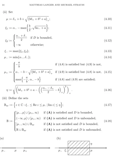
In the following definition we introduce a set, B, in which the quadratic nu-merical range and the spectrum of Mare contained, as we shall show in Proposi-tion 4.10 and Theorem 4.13 below. Moreover, we introduce condiProposi-tion (A) under which W2(M) and σ(M) are contained in
R. Some comments concerning these definitions are given in Remark 4.6; see also Figure 1, which shows the set Bwhen D is bounded.
Definition 4.5. Assume that Assumption 2.1 is satisfied. Let a ∈ R, b ≥ 0 such that (2.3) holds and let α−, δ+ as in (2.1). Moreover, if D is bounded, set
δ−:= minσ(D); otherwise setδ−:=−∞. (i) We say that condition(A)is satisfied if
bδ++b2+a≤0 and b >0 (4.8)
or
α−−δ+
2 ≥b+
q
bδ++b2+a
(ii) Set
µ:=δ++b+ q
bδ++b2+a
+; (4.10)
ξ1:=α−−max b
2,
p
bα−+a
; (4.11)
ξ2:=
α−+δ−
2 ifD is bounded,
−∞ otherwise;
(4.12)
ξ−:= max{ξ1, ξ2}; (4.13)
µ−:= min{α−, δ−}; (4.14)
µ+:=
−a
b if (4.8) is satisfied but (4.9) is not, α−−b−
q
bδ++b2+a
+ if (4.9) is satisfied but (4.8) is not,
maxn−a
b, α−−b
o
if (4.8) and (4.9) are satisfied;
(4.15)
η:=
s
bδ++b2+a−
α
−−δ+
2 −b
+ 2
+
. (4.16)
(iii) Define the sets Bnr:=
n
z∈C:ξ−≤Rez≤µ, |Imz| ≤η
o
; (4.17)
B:=
[µ−, µ]∪[µ+,∞) if (A) is satisfied andD is bounded,
(−∞, µ]∪[µ+,∞) if (A) is satisfied andD is unbounded,
[µ−,∞)∪Bnr if (A) is not satisfied andD is bounded,
R∪Bnr if (A) is not satisfied andD is unbounded.
(4.18)
(a)
-µ µ+
µ−
(b)
-µ− ξ− µ
[image:14.595.112.484.85.592.2]η
Figure 1. The setBwhenDis bounded; (a) shows the case when (A) is satisfied; (b) shows the case when(A) is not satisfied.
Remark 4.6.
(i) If B 6= 0, then a6= 0 or b 6= 0 and therefore the right-hand side of (4.9) is positive andµ > δ+(note that a >0 ifb= 0).
(ii) If B6= 0 and the first inequality in (4.8) is satisfied, then automaticallyb >0 (sincea >0 ifb= 0).
(iii) Assume that(A) is satisfied and thatB6= 0. Then
In particular, the spectra ofAandD must be separated. The inequalities in (4.19) are true because of the following considerations. If (4.8) holds, then b >0, and from (i), (4.8) and (2.5), we obtain
δ+< µ=δ++b≤ −
a
b ≤µ+≤α−.
If (4.9) holds, then
δ+< µ≤
α−+δ+
2 ≤µ+≤α−. (4.20) If (4.9) holds but (4.8) does not, thenµ+< α−. If the first inequality in (4.8) or the inequality in (4.9) is strict, then µ < µ+. Moreover, if (4.9) is strict,
then
δ+< µ <
α−+δ+
2 < µ+≤α−.
(iv) If (4.8) is satisfied, it can happen thatµ+ =α−. Consider, for instance the situation whenα− = 0 and (2.3) holds witha= 0 and b >0. Thenµ+= 0.
On the other hand, if (4.8) is not satisfied but (4.9) is, then alwaysµ+< α−.
(v) The numberµ+ can also be characterised as
µ+= max
µ(1)+ , µ(2)+
where
µ(1)+ :=
−a
b if (4.8) is satisfied,
−∞ otherwise,
µ(2)+ :=
α−−b−q bδ++b2+a
+ if (4.9) is satisfied,
−∞ otherwise.
(vi) IfB is “small”, i.e.aandbare small, then in generalξ1gives the better lower
bound for the real part of non-real elements fromB. If D is bounded andB is “large”, thenξ2 gives the better bound as it is independent ofB.
(vii) It is elementary to see thatη= 0 if and only if (A)is satisfied; moreover,
η=
0 if (A) is satisfied,
p
bδ++b2+a if (A) is not satisfied andb≥
α−−δ+
2 ,
s
bα−+a− α
−−δ+
2
2
if (A) is not satisfied andb < α−−δ+ 2 . (viii) If B is bounded, then one can choosea=kBk2 andb= 0, and hence
µ=δ++kBk, ξ1=µ+=α−− kBk, (4.21)
η=
s
kBk2−
α−−δ+
2
+ 2
+
. (4.22)
Before we prove that BcontainsW2(M) andσ(M), we need some lemmas. Lemma 4.7. Letb≥0 anda, t, δ∈R, and assume that
t −δ
2
2
Then
bδ+b2+a≥0 and t−δ 2 ≤b+
p
bδ+b2+a . (4.24)
If strict inequality holds in (4.23), then the inequalities in (4.24) are also strict. Proof. Relation (4.23) is equivalent to
t2−2(δ+ 2b)t+δ2−4a≤0. The zeros of the polynomial inton the left-hand side are
t±:=δ+ 2b±
p
(δ+ 2b)2−δ2+ 4a=δ+ 2b±2pbδ+b2+a .
If (4.23) is satisfied, then the discriminant is non-negative and t− ≤t≤t+, which
yields (4.24). If the inequality in (4.23) is strict, then t− < t < t+ and hence the
discriminant is strictly positive. Lemma 4.8. Assume that (A) is satisfied and let x ∈ dom(a)\{0} and y ∈
dom(d)\{0}. Thenλ± xy∈R. Moreover, if (4.8)holds, then
λ+ x
y
≥ −a
b ; (4.25)
if (4.9)holds, then λ+
x y
≥α−−b−q bδ++b2+a
+. (4.26)
Proof. Letα,β andδbe as in (4.1). Suppose thatλ± xy∈/R. Then, by (4.2) and (4.3), we have
α−δ
2
2
<|β|2≤bα+a.
This, together with Lemma 4.7, implies that bδ+b2+a >0 and α−δ
2 < b+
p
bδ+b2+a .
By the definition ofα− andδ+ we obtain
bδ++b2+a >0 and
α−−δ+
2 < b+
p
bδ++b2+a ,
which is a contradiction to (A). Henceλ± xy∈R. It follows again from (4.2) and (4.3) that
λ+ x
y
≥ α+δ
2 +
s α−δ
2
2
−bα−a . (4.27) Assume that (4.8) holds. Then
bδ+b2+a≤0 (4.28) and b >0. Define the function
f(t) := t+δ 2 +
s t
−δ 2
2
−bt−a , t∈R,
which is real-valued by (4.28). Its derivative is f0(t) = 1
2 +
t−δ
2 −b
2
q
t−δ
2 2
−bt−a
= f(t)−(δ+b) 2
q
t−δ
2 2
−bt−a ,
increasing on R and f(t)> δ+b for allt ∈ R. Relations (2.5) and (4.28) imply that
α≥α− ≥ − a
b ≥δ+b≥δ. Hence, by (4.27),
λ+ x
y
≥f(α)≥f−a
b
=−a
b , i.e. (4.25) holds.
Now assume that (4.9) is satisfied. Note first that, for r, s∈Rsuch that r≥0 and r≥s, one has √
r−s≥√r−√s+,
which is easy to see. From this and the relation α−δ2 ≥bit follows that
λ+ x
y
≥ α+δ
2 +
s α−δ
2
2
−bα−a
= α+δ 2 +
s
α−δ 2 −b
2
−(bδ+b2+a)
≥ α+δ
2 +
s α−δ
2 −b
2 −p
(bδ+b2+a) +
=α−b−p(bδ+b2+a) +
≥α−−b−
q
bδ++b2+a
+,
i.e. (4.26) holds.
Lemma 4.9. Let x∈dom(a)\{0} andy ∈dom(d)\{0} and letµ be as in (4.10). Then
Reλ−
x y
≤µ.
Proof. Letx∈dom(a)\{0} andy∈dom(d)\{0} and letα,β andδbe as in (4.1). Then
λ−:=λ−
x
y
=α+δ 2 −
s α−δ
2
2 − |β|2
and (4.3) is valid.
Let us first consider the case when
t−δ 2
2
≤bt+a for some t≥α.
It follows from Lemma 4.7 that the inequalities in (4.24) hold, which imply Reλ−≤
α+δ 2 ≤
t+δ
2 ≤δ+b+
p
bδ+b2+a ≤δ++b+
p
bδ++b2+a =µ.
Now we consider the case when
t−δ
2
2
> bt+a for allt≥α. (4.29) It follows from (4.29) and (4.3) thatλ−∈Rand
λ−≤ α+δ
2 −
s α−δ
2
2
Define the function
f(t) := t+δ 2 −
s t
−δ 2
2
−bt−a
for such t for which the expression under the square root is non-negative, i.e. ei-ther dom(f) = R or dom(f) = (−∞, t−]∪[t+,∞) where t± are the zeros of the polynomial under the square root:
t±=δ+ 2b±2
p
bδ+b2+a .
The derivative of f is
f0(t) =1 2 −
t−δ
2 −b
2
q
t−δ
2 2
−bt−a
= δ+b−f(t) 2
q
t−δ
2 2
−bt−a ,
which implies that
f0(t)>0 ⇐⇒ f(t)< δ+b. (4.31) If a=b= 0, then β = 0 and the assertion is clear since thenλ− = min{α, δ}. So assume thata6= 0 orb6= 0. Thenf is not constant. It follows from (4.31) that the sign off0 is constant on each interval in the domain off. Let us first consider the case when dom(f) =R. Sincef(t)→ −∞ast→ −∞, we havef(t)< δ+bfor all t∈Rand hence (with (4.30))
λ−≤f(α)< δ+b≤δ++b≤µ.
Now consider the case when dom(f)6=R. It follows from (4.29) that α∈[t+,∞).
Moreover,
f(t+) =
t++δ
2 =δ+b+
p
bδ+b2+a ≥δ+b,
which, by (4.31), implies that f0(t)≤0 on (t+,∞). Hence (again with (4.30))
λ−≤f(α)≤f(t+) =δ+b+ p
bδ+b2+a ≤δ ++b+
p
bδ++b2+a =µ,
which proves the assertion also in this case. The next proposition shows that the closure of the quadratic numerical range is contained in B.
Proposition 4.10. Suppose that Assumption2.1is satisfied. LetMbe the operator as in Theorem2.4,W2(M)as in Definition4.1 and
B,µ,µ+ as in Definition4.5.
ThenW2(M)⊂
B.
Moreover, if (A) is satisfied, then W2(M)⊂Rand λ−
x y
≤µ, λ+
x y
≥µ+ for x∈dom(a)\{0}, y∈dom(d)\{0}. (4.32)
Proof. Since B is closed, it suffices to prove thatW2(M)⊂
B. Letz ∈ W2(M). Then there exist x ∈ dom(a)\{0} and y ∈ dom(d)\{0} such that z = λ+ xy or
z=λ− xy. Letα, β andδbe as in (4.1).
First assume thatz∈R. If condition(A)is satisfied, then, by Lemmas 4.8 and 4.9, we have either z=λ+ xy
≥µ+ or z=λ− xy≤µ, which also shows (4.32). If D is bounded, then
z≥λ−
x
y
≥α+δ
2 −
α−δ 2
Now assume thatz /∈R. Using (4.3) and the relationt2≥((t)
+)2 fort∈Rwe obtain for the imaginary part ofz that
|Imz|=
s
|β|2− α−δ
2
2
+ ≤
s
bα+a−
α−δ
2
2
+
=
s
bδ+b2+a− α
−δ 2 −b
2
+
≤ s
bδ+b2+a−
α−δ
2 −b
+ 2
+
≤ s
bδ++b2+a−
α−−δ+
2 −b
+ 2
+
.
The upper bound for Rez follows directly from Lemma 4.9. For the lower bound observe that
0>
α −δ 2
2
− |β|2≥ α
−δ 2
2
−bα−a.
Hence bα+a >0 and
α−δ 2 <
√
bα+a , which implies that
Rez=α+δ 2 > α−
√
bα+a . (4.33) If b = 0, then the right-hand side of (4.33) is bounded from below by α−−√a, which is equal to ξ1 in that case. For the case b >0 we consider the function
f(t) :=t−√bt+a , t∈h−a
b,∞
,
which attains its minimum att0:= b4−ab . Ift0≤α−, then min
t∈[α−,∞)
f(t) =f(α−) =α−−
p
bα−+a . Ift0> α−, then
min t∈[α−,∞)
f(t) =f(t0) =t0−
b
2 > α−− b 2. Hence Rez≥ξ1 also in this case.
IfD is bounded, then one also hasδ≥δ− and hence Rez= α+δ
2 ≥
α−+δ− 2 =ξ2.
This shows that Rez≥ξ− in all cases and hencez∈B. Next we need an auxiliary lemma before we prove the spectral inclusion. For a similar result for certain diagonally dominant block operator matrices we refer to [29, Theorem 4.2].
Lemma 4.11. Suppose that Assumption2.1is satisfied and letz∈C\(δ+, δ++b0).
Thenz /∈W2(M)implies that M −z has closed range.
Proof. We show the contraposition. Let z ∈ C\(δ+, δ++b0) and suppose that
ran(M−z) is not closed. Then,z∈σapp(M), i.e. there exists a sequence (xn, yn)T ∈
dom(M) with (M −z)
x
n yn
see [16, Theorem IV.5.2]. We have to show that z∈W2(M).
If dimH1= 1 or dimH2 = 1, thenB is bounded, and hence [29, Corollary 4.3] implies that z ∈ W2(M). If A is bounded, then B is bounded, and again z ∈
W2(M). For the rest of the proof assume that dimH1≥2, dimH2≥2 and that
A is unbounded.
It follows from (2.12) and (2.13) that
a[xn]−zkxnk2+hyn, B∗xni →0, (4.34)
−hB∗xn, yni+d[yn]−zkynk2→0. (4.35)
First we consider the case whenz∈C\R. Taking the imaginary parts of the left and the right-hand sides of (4.34) and (4.35) we obtain
−Imzkxnk2+ Imhyn, B∗xni →0 and −ImhB∗xn, yni −Imzkynk2→0.
If we take the difference and observe that Imz 6= 0, we get kxnk − kynk →0 and thus
kxnk → √1
2 and kynk → 1
√
2 . (4.36) Lemma 3.5 (i) implies that a[xn] andhB∗xn, yniare bounded. By (4.35) alsod[yn] is bounded. From (4.34), (4.35) and (4.36) it follows that
Mxn,yn−z
kxnk kynk !
=
a[xn]−zkxnk2+hyn, B∗xni
kxnk
−hB∗xn, yni+d[yn]−zkynk2 kynk
→0. (4.37)
Since all entries ofMxn,yn are bounded, (4.37) and (4.36) imply that
det(Mxn,yn−z)→0.
Hence there exists a sequence zn ∈σ(Mxn,yn)⊂W
2(M) such thatzn→z, which
shows that z∈W2(M).
Now letz∈R. Taking the sum of the real parts of the left-hand sides of (4.34) and (4.35) we obtain
a[xn]−zkxnk2+d[yn]−zkynk2→0. Ifz < µ−, i.e.D is bounded andz < α− andz < δ−, then
a[xn]−zkxnk2+d[yn]−zkynk2≤(α−−z)kxnk2+ (δ−−z)kynk2
≤maxα−−z, δ−−z kxnk2+kynk2
= maxα−−z, δ−−z <0, which is a contradiction.
If δ− ≤z ≤δ+, then z ∈W(D); ifz ≥α−, then z ∈W(A) since we assumed that Ais unbounded. In both cases it follows from Lemma 4.4 thatz∈W2(M).
Finally, assume that z ∈ (δ+ +b0, α−). Since z ∈ U in this case, we have lim infn→∞kxnk > 0 by Lemma 3.5 (iii). Ifynk → 0 for a subsequenceynk, then
(4.34) implies that a[xnk]−zkxnkk
2→0, which is a contradiction to the fact that kxnkk →1 and z < α−. Hence also lim infn→∞kynk >0 and we can argue as in
the case z∈C\Rto obtain thatz∈W2(M). The next proposition shows that, essentially, the spectrum ofMis contained in the closure of the quadratic numerical range. Only in the interval (δ+, δ++b0) we
Proposition 4.12. Suppose that Assumption 2.1 is satisfied and let M be the operator as in Theorem 2.4. Moreover, letz ∈ C\(δ+, δ++b0). Then z ∈ σ(M)
implies that z∈W2(M).
Proof. Assume that z /∈ W2(M). It follows from Lemma 4.11 that ran(M −z)
is closed. Moreover, Lemma 4.3 applied to M and M∗ yields nul(M −z) = 0 and nul(M∗−z) = 0. The latter implies that def(M −z) = 0; see, e.g. [16, Theorem IV.5.13]. Hencez∈ρ(M).
The next theorem shows that the spectrum ofMis contained inB.
Theorem 4.13. Suppose that Assumption2.1is satisfied, letMbe the operator as in Theorem2.4and letBas in(4.18). Thenσ(M)⊂B. In particular, if condition (A) is satisfied, then σ(M)⊂R.
Proof. Let z ∈ σ(M). If z ∈ C\(δ+, δ++b0), then z ∈ W2(M)⊂ B by Propo-sitions 4.12 and 4.10. If z ∈ (δ+, δ+ +b0), then z ∈ B since µ− ≤ δ+ and
δ++b0≤δ++b≤µ.
When B is a bounded operator, then η, which bounds the imaginary parts of spectral points, is given by (4.22); this was proved in [29, Theorem 5.5 (iii)].
The above theorem shows that the spectrum is real provided the spectra of the diagonal components are sufficiently separated and B is not “too large”. As the following result shows, this can be particularly straightforward whenBis bounded; see also [30, Proposition 2.6.8] and [29, Theorem 5.5].
In the next corollary, which follows immediately from Theorem 4.13 and Re-mark 4.6 (viii), we consider the situation whenB is bounded. The estimate for the imaginary part in (4.39) was also proved in [29, Theorem 5.5]. A slightly better enclosure for σ(M) than (4.38) was obtained in [3, Theorem 5.8] and [4, Theo-rem 5.4].
Corollary 4.14. Suppose that Assumption 2.1is satisfied and thatB is bounded. If
kBk ≤ α−−δ+
2 , then
σ(M)⊂ −∞, δ++kBk
∪
α−− kBk,∞
. (4.38) Otherwise,
σ(M)⊂R∪
(
z∈C\R: α−− kBk ≤Rez≤δ++kBk,
|Imz| ≤ r
kBk2−α−−δ+
2
+ 2
)
.
(4.39)
If D is bounded with δ− = minσ(D), then (−∞, δ−) ⊂ρ(M) and Rez ≥ α−+2δ− forz∈σ(M)\R.
Proof. SinceB is bounded, we can chose a=kBk2andb= 0. Under our
assump-tions the inequality (4.9) is satisfied. Hence (4.38) holds by Theorem 4.13 and the
definition of B.
Remark 4.16. Let us consider the family of operators
Mt:=
A tB
−tB∗ D
, t∈[0,∞),
which was also studied in [21]. Clearly, if Assumption 2.1 is satisfied for t = 1, then it is satisfied for all t∈ [0,∞). Ifδ+ < α−, i.e. the spectra ofA and D are
separated, then there exists a t0 > 0 such that, for t ∈ [0, t0], condition (A) is
satisfied and hence σ(Mt)⊂R. Ifδ+ ≥α−, it may happen that the spectrum of
Mis non-real for every positivet.
Ifδ+< α−, then, in general, the gap (δ+, α−) in the spectrum closes from both endpoints with increasingt. However, if, e.g.α− = 0 anda= 0,b >0 in (2.3), then µ+ =α−as long as (4.8) is satisfied, i.e. the gap closes only from the left endpoint. If D is bounded andδ− = minσ(D), then for allt∈[0,∞), the setσ(Mt)∩R is bounded from below by min{α−, δ−}and the real parts of points fromσ(Mt)\R are bounded from below by α−+δ−
2 .
In the next section we characterise elements from σ(M) in the interval (µ,∞) with variational principles. Since the proof uses the Schur complement, we must ensure that S and M have the same essential spectrum in (µ,∞). Note that (µ,∞)⊂Uand henceS(λ) is well defined forλ∈(µ,∞).
Theorem 4.17. Suppose that Assumption 2.1 is satisfied, let M be the operator as in Theorem 2.4, letS be its Schur complement and letµ be as in (4.10). Then
σess(S)∩(µ,∞) =σess(M)∩(µ,∞). (4.40)
Proof. Let z∈σess(S)∩(µ,∞). Since 0∈σess(S(z)) and S(z) is self-adjoint, the
operator S(z) is not semi-Fredholm with nul(S(z))<∞. By [10, Theorem IX.1.3] there exists a singular sequence for S(z) corresponding to 0, i.e. there existxn ∈ dom(S(z)),n∈N, such that
kxnk= 1, S(z)xn→0, xn*0. Set
yn := (D−z)−1B∗xn, wn:=
xn yn
, and wnˆ := wn
kwnk.
From Lemma 3.4 (i) we obtain that ˆwn∈dom(M) and (M −z) ˆwn=
1
kwnk
S(z)xn
0
→0;
note thatkwnk ≥1. Moreover, foruin the dense set dom(B(D−z)−1) we have hyn, ui=
xn, B(D−z)−1u →0.
Since yn is bounded by Lemma 3.5 (i), we have yn * 0 and therefore ˆwn * 0. Hence ˆwn is a singular sequence forMcorresponding to z. Again from [10, Theo-rem IX.1.3] we obtain thatz∈σess(M). This shows the inclusion “⊂” in (4.40).
Now let z ∈ σess(M)∩(µ,∞) and suppose that z /∈ σess(S). It follows from
Theorem 3.6 thatz∈σ(S) and that
0<nul(S(z)) = nul(M −z)<∞. (4.41) Since S(z) is self-adjoint, we also have 0∈ σdis(S(z)). Suppose thatM −z has
Hence ran(M −z) is not closed. Therefore, by [16, Theorem IV.5.2], there exists a sequence of vectors (xn, yn)T ∈dom(M) with
x
n yn
⊥ker(M −z) and kxnk2+kynk2= 1 for eachn∈N (4.42) such that
u
n vn
:= (M −z)
x
n yn
= (A−ν) xn+ (A−ν)
−1Byn
+ (ν−z)xn
−B∗x
n+ (D−z)yn
! →0.
Let P be the orthogonal projection fromH1 onto ker(S(z)), set ˜xn = (I−P)xn and let ˜S(z) be the restriction of S(z) to the Hilbert space (I−P)H1, which has
a bounded inverse since 0 ∈ σdis(S(z)). Set ξn := ˜S(z)−1x˜n. Since B∗S(z)˜ −1 is a bounded operator by the closed graph theorem, the assumptions on ξn in Lemma 3.5 (iii) are satisfied. The latter implies that
kx˜nk2=s(z)
xn,S(z)˜ −1x˜n
→0.
Since ker(S(z)) is finite-dimensional, there exists a subsequence xnk such that xnk → x ∈ ker(S(z)). It follows from Lemma 3.5 (iv) that x ∈ dom(a) and
B∗x nk →B
∗x. Hence
x
nk
ynk
→
x
(D−z)−1B∗x
∈ker(M −z)
by Lemma 3.4. As this contradicts (4.42), we have z∈σess(S). Hence the reverse
inclusion in (4.40) is also shown. Corollary 4.18. If Ahas compact resolvent, then (µ,∞)∩σess(M) =∅.
Proof. In view of Theorem 4.17, it is sufficient to show that (µ,∞)∩σess(S) =∅. Letz∈(µ,∞) andx∈dom(a). It follows from (3.2) that
(D−z)−1B∗x, B∗x ≤
b z−δ+
a[x] + a z−δ+
kxk2,
Since z−δ+ > b, this, together with [16, Theorem VI.3.4], implies that S(z) has
compact resolvent.
Recall that under the extra assumption 2.1.(I) more can be said aboutσess(M);
see Proposition 3.7.
5. Variational Principles
In this section we prove variational principles that characterise eigenvalues of the operator Mand the Schur complementS in a certain interval. The functionals in these variational principles are connected either with the Schur complement or the quadratic numerical range of the operator M.
First we recall a property of operator functions that was used in [31, Lemma 2] by A. Virozub and V. Matsaev for functions whose values are bounded operators; see also, e.g. [20, 23]. In [27] this property was introduced for certain functions whose values are unbounded operators. Here we formulate it for families of quadratic forms and apply it then to holomorphic operator functions of type (B).
Definition 5.1. Let ∆ ⊂ R be an interval and let t(λ), λ ∈ ∆, be a family of closed symmetric quadratic forms such that dom(t(λ)) is independent of λ and such that t(·)[x] is differentiable for eachx∈dom(t(λ)). We say thatt(·) satisfies the condition (VM−)on the interval ∆ if, for each compact subinterval I ⊂ ∆, there existε, δ >0 such that, for allλ∈I and allx∈dom(t(λ)),
t(λ)[x]
≤εkxk
2 =
The condition implies in particular that ifλ0is an inner point of ∆ and|t(λ0)[x]|
is small enough, thent(·)[x] must have a zero close toλ0.
Lemma 5.2. Lets(λ),λ∈U, be the quadratic forms from Definition3.1associated with the Schur complement of the operator M and letµ be as in (4.10). Then s
satisfies the condition (VM−)on the interval(µ,∞). Proof. First note that
s(λ)[x] =a[x]−λkxk2−
(λ−D)− 1
2B∗x2, (5.2)
s0(λ)[x] =−kxk2+
(λ−D)−1B∗x 2
. (5.3)
Let ε > 0 be arbitrary for the moment, let λ ∈ (µ,∞) and let x ∈ dom(a) = dom(s(λ)) such that|s(λ)[x]| ≤εkxk2. It follows from (2.3) and (5.2) that
(λ−D)− 1
2B∗x2≤kB
∗xk2
λ−δ+
≤ ba[x] +akxk 2
λ−δ+
=b s(λ)[x] +λkxk
2+
(λ−D)− 1
2B∗x2+akxk2
λ−δ+
.
Rearranging this inequality we obtain (λ−δ+−b)
(λ−D)− 1
2B∗x2≤bs(λ)[x] + (bλ+a)kxk2≤(bε+bλ+a)kxk2.
Sinceλ > δ++b, we have
s0(λ)[x]≤ −kxk2+
(λ−D)− 1
22(λ−D)− 1 2B∗x2
≤
−1 + 1 λ−δ+
·bε+bλ+a
λ−δ+−b
kxk2= g(λ) +h(λ)ε kxk2,
where
g(λ) :=−1 + bλ+a (λ−δ+)(λ−δ+−b)
, h(λ) := b
(λ−δ+)(λ−δ+−b)
.
Moreover,g(λ)<0 if and only ifλ2−2(δ++b)λ+δ2++bδ+−a >0; it is easily seen
that the latter inequality is true forλ∈(µ,∞). Now letIbe a compact subinterval of (µ,∞). Since g is continuous on (µ,∞) and I is compact, there exists a c <0 such that g(λ)≤c forλ∈I. Chooseε >0 so small that εh(λ)≤c/2 for λ∈ I. Then, with δ:=c/2, we haves0(λ)[x]≤ −δkxk2 forλ∈I.
The previous lemma implies that if the function s(·)[x], for x ∈ dom(a)\{0}, has a zero, then the derivative is negative at this zero. In particular, for each x∈dom(a)\{0}the functions(·)[x] is decreasing at value zero (in the terminology of [7] and [12]) and hence has at most one zero in (µ,∞). Moreover,s(λ)[x]→ −∞
as λ→ ∞.
Next we define a generalised Rayleigh functional, which is used in the variational principle below. This functional generalises the Rayleigh quotient for linear oper-ators to the situation of an operator function; for more general operator functions it has been defined in [7] and [12].
Definition 5.3. We define the generalised Rayleigh functional p: dom(a)\{0} →
R∪ {−∞}as follows
p(x) =λ0 ifs(λ0)[x] = 0 for aλ0∈(µ,∞),
p(x) =−∞ ifs(λ)[x]<0 for allλ∈(µ,∞).
Before we formulate the next theorem we introduce another notation that is needed. Definition 5.5. For a self-adjoint operator T denote byκ−(T) the dimension of the spectral subspace for T corresponding to the interval (−∞,0).
The next theorem contains a variational principle for eigenvalues of M in the interval (µ,∞). Note that there is a shift in the index: in general, the index of the eigenvalue does not match the dimension of the corresponding subspace in the variation. For boundedA,B andD a similar but slightly weaker result was proved in [7, §4.3].
Theorem 5.6. Suppose that Assumption2.1is satisfied, let Mbe the operator as in Theorem2.4, letµbe as in (4.10)and let pandκ− be as in Definitions 5.3and 5.5. Assume that
∃γ∈(µ,∞) such that κ−(S(γ))<∞. (5.4) Then
µ < λe:= (
inf σess(M)∩(µ,∞) ifσess(M)∩(µ,∞)6=∅,
∞ otherwise.
(5.5)
Moreover,σ(M)∩(µ, λe)is at most countable, consists of eigenvalues only and has
λe as only possible accumulation point.
Let γ0 ∈ (µ, λe) be arbitrary and let (λj)Nj=1, N ∈ N0∪ {∞}, be the finite or
infinite sequence of eigenvalues of M in the interval [γ0, λe) in non-decreasing
order and repeated according to multiplicities. Then
κ:=κ−(S(γ0))<∞ (5.6)
and
λn= min L⊂dom(a) dimL=κ+n
max
x∈L\{0} p(x) = maxL⊂H
dimL=κ+n−1
inf x∈dom(a)\{0}
⊥L
p(x) (5.7)
for n∈ N, n≤N. Moreover, if N is finite andH1 is infinite-dimensional, then λe<∞and
λe= inf
L⊂dom(a) dimL=κ+n
max
x∈L\{0} p(x) = L⊂Hsup
dimL=κ+n−1
inf x∈dom(a)\{0}
x⊥L
p(x) (5.8)
forn > N.
Proof. Note first that σ∗(M)∩(µ,∞) =σ∗(S)∩(µ,∞) forσ∗ =σ, σp, σess; see
Theorems 3.6 and 4.17. Lemma 3.2 implies that the Schur complement S is a holomorphic operator family of type (B). Moreover,Ssatisfies the condition(VM−) on (µ,∞) by Lemma 5.2. Hence the assumptions (i)–(v) in [12,§2] are satisfied.
Suppose that λe =µ. Then, for everyε >0, there exists a λ∈(µ, µ+ε) such
that λ∈σess(S). This, together with [12, Lemma 2.9], implies thatκ−(S(t)) =∞ for all t > λ, a contradiction. Hence λe > µ. Now almost all remaining assertions
follow immediately from [12, Theorem 2.1]. We only have to show that λe<∞if
N <∞and dimH1=∞. Suppose thatλe=∞. Then, by [12, Theorem 2.1]
inf L⊂dom(a) dimL=κ+n
max
x∈L\{0} p(x) =∞
forn > N, i.e. for everyL ⊂dom(a) with dimL> κ+None has maxx∈L\{0}p(x) =
∞. By [12, Lemma 2.8] the maximum is attained and thereforep(x) =∞for some x∈ L. However, this is a contradiction to the definition ofpin our case and hence
λe<∞.
Corollary 5.7. Suppose that Assumption2.1is satisfied, letMbe the operator as in Theorem2.4, letµbe as in (4.10)and let pandκ− be as in Definitions 5.3and 5.5. Assume thatA has compact resolvent and thatH1 is infinite-dimensional.
Then κ−(S(γ)) < ∞ for every γ ∈ (µ,∞). Moreover, σess(M)∩(µ,∞) = ∅ and henceλe=∞. Further,σ(M)∩(µ,∞)consists of infinitely many eigenvalues
(i.e.N =∞), which accumulate only at∞, and (5.7)holds for alln∈N.
Proof. It follows from Lemma 3.2 and the proof of Corollary 4.18 that S(γ) is bounded from below and has compact resolvent. This implies that κ <∞. More-over, σess(M)∩(µ,∞) =∅by Corollary 4.18. Finally, N =∞because otherwise
λe<∞by Theorem 5.6.
The next simple lemma is used below and was proved in [21, Lemma 3.5] for boundedB.
Lemma 5.8. Let x ∈ dom(a)\{0} such that B∗x 6= 0 and let λ ∈ U. With y:= (D−λ)−1B∗xwe have
det Mx,y−λ
=
B∗x,(D−λ)−1B∗xs(λ)[x]
kxk2kyk2 .
Proof. Clearly,y6= 0. From the definition ofMx,y we obtain
kxk2kyk2det M
x,y−λ
= a[x]−λkxk2
d[y]−λkyk2
+hy, B∗xihB∗x, yi
= a[x]−λkxk2
B∗x,(D−λ)−1B∗x
+(D−λ)−1B∗x, B∗xB∗x,(D−λ)−1B∗x =
B∗x,(D−λ)−1B∗x
s(λ)[x],
which proves the assertion.
In the next proposition we consider the case when one of the inequalities (4.8), (4.9) is strict. Then the index shift κis equal to 0 for appropriateγ0.
Proposition 5.9. Suppose that Assumption2.1 is satisfied, letMbe the operator as in Theorem 2.4, let a∈R,b≥0 be such that (2.3) is satisfied and letµ,µ+ be
as in (4.10) and (4.15), respectively. Assume that
bδ++b2+a <0 or
α−−δ+
2 > b+
q
bδ++b2+a
+. (5.9)
Then
δ+< µ < µ+≤α−, (5.10) and for each γ∈(µ, µ+)there exists ac >0 such that
s(γ)[x]≥ckxk2, x∈dom(a), (5.11)
and hence κ−(S(γ)) = 0.
Proof. The inequalities in (5.10) follow from Remark 4.6 (iii). Letγ∈(µ, µ+) and
x ∈ dom(a)\{0}. We first show that s(γ)[x] > 0. If B∗x = 0, then s(γ)[x] =
a[x]−γkxk2>0 sinceγ < α−. Now assume thatB∗x6= 0. Sety:= (D−γ)−1B∗x. From Proposition 4.10 we obtain
λ−
x
y
≤µ < γ < µ+≤λ+ x
y
Now Lemma 5.8 implies that 0>
γ−λ+ x
y
γ−λ−
x
y
= det Mx,y−γ
=
B∗x,(D−γ)−1B∗x
s(γ)[x]
kxk2kyk2 .
Sinceγ > δ+, this shows thats(γ)[x]>0. Hence the operatorS(γ) is non-negative.
Further, (µ, µ+) ⊂ρ(M) by Theorem 4.13 and therefore 0∈ ρ(S(γ)) by
The-orem 4.17. This proves that S(γ) is uniformly positive, i.e. (5.11) holds and
κ−(S(γ)) = 0.
In Theorem 5.12 below we prove a variational principle with the functional λ+.
To this end we need some lemmas to rewritep(x) in terms ofλ+.
Lemma 5.10. Let x∈dom(a)and assume that B∗x6= 0. If s(λ)[x]≤0 for some λ∈(µ,∞), then
λ+
x
(D−λ)−1B∗x
≤λ. (5.12)
If s(λ)[x] = 0, then there is equality in (5.12).
Proof. Sety:= (D−λ)−1B∗x, which is non-zero. From Lemma 5.8 we obtain
det Mx,y−λ
=
B∗x,(D−λ)−1B∗x
s(λ)[x]
kxk2kyk2 ≥0
sinceλ > δ+. By Lemma 4.9 we haveλ− xy≤µ < λ, which implies thatλ+ xy
≤λ. Ifs(λ)[x] = 0, then det(Mx,y−λ) = 0 and henceλ+ xy
=λ.
Lemma 5.11. Let x∈dom(a)\{0}.
(i) If s(λ0)[x] = 0for someλ0∈(µ,∞), i.e.λ0=p(x), then
λ±
x
y
∈R for all y∈dom(d)\{0} and
min y∈dom(d)\{0}λ+
x
y
=λ0. (5.13)
(ii) If s(λ)[x]<0for all λ∈(µ,∞), i.e.p(x) =−∞, then inf
y∈dom(d)\{0}Reλ+
x
y
≤µ. (5.14)
Proof. IfB∗x= 0, thens(λ)[x] =a[x]−λkxk2and
λ+ x
y
= max
a[x] kxk2,
d[y]
kyk2
for all y∈dom(d)\{0}.
Sinced[y]/kyk2≤δ
+≤µ, the assertion follows in both cases (i) and (ii).
For the rest of the proof we assume thatB∗x6= 0.
(i) Suppose that s(λ0)[x] = 0 for someλ0∈(µ,∞). For anyy∈dom(d)\{0}we
have
|hy, B∗xi|2=
(λ0−D) 1
2y,(λ0−D)− 1 2B∗x2
≤(λ0−D) 1
2y2(λ0−D)− 1 2B∗x2
= (d−λ0)[y]