Debris re-entry modeling using high dimensional derivative based uncertainty quantification

AAS 15-557

DEBRIS RE-ENTRY MODELING USING HIGH DIMENSIONAL

DERIVATIVE BASED UNCERTAINTY QUANTIFICATION

Piyush M. Mehta

_{, Martin Kubicek}

_{, Edmondo Minisci}

_{, and Massimiliano}

Vasile

Well-known tools developed for satellite and debris re-entry perform break-up and trajectory simulations in a deterministic sense and do not perform any uncertainty treatment. In this paper, we present work towards implementing uncertainty treatment into a Free Open Source Tool for Re-entry of Asteroids and Space Debris (FOSTRAD). The uncertainty treatment in this work is limited to aerodynamic trajectory simulation. Results for the effect of uncertain parameters on trajectory simulation of a simple spherical object is presented. The work uses a novel uncertainty quantification approach based on a new derivation of the high dimensional model representation method. Both aleatoric and epistemic uncertainties are considered in this work. Uncertain atmospheric parameters considered include density, temperature, com-position, and free-stream air heat capacity. Uncertain model parameters considered include object flight path angle, object speed, object mass, and direction angle. Drag is the only aerodynamic force considered in the planar re-entry problem. Results indicate that for initial conditions corresponding to re-entry from a circular orbit, the probabilistic distributions for the impact location are far from the typically used Gaussian or ellipsoids and the high prob-ability impact location along the longitudinal direction can be spread over∼2000 km, while the overall distribution can be spread over∼4000 km. High probability impact location along the lateral direction can be spread over∼400 km.

INTRODUCTION

Background and Motivation

Space Situational Awareness is quickly becoming imperative for nations around the world, especially those with space capabilities and assets. As the low Earth orbit (LEO) debris and spacecraft population that have exceeded their operational lifetime rises each year, the rate at which objects re-enter the Earth0s atmosphere will also steadily rise. Most of these objects will probably not reach the ground for impact; however, large objects like rocket bodies, ENVISAT, or the ISS have a high probability of surviving the harsh re-entry environment. These large re-entering objects can retain a significant fraction of their orbital energy when they impact, likely causing damage within a populated area. The impact location of an object re-entering the atmosphere can be altered by uncertainties in initial conditions, atmospheric characteristics, and object properties, as well as break-up/fragmentation events. Therefore, it is important to have an accurate estimate of not just the deterministic impact location but also the statistic ground footprint due to the uncertainties involved. Current re-entry modeling tools used by space agencies are deterministic, proprietary, and are not freely available to the research community1,2,3.

The Free Open Source Tool for Re-entry of Asteroids and Space Debris (FOSTRAD) is a re-entry tool development effort at the University of Strathclyde to overcome the non-freely available, non-open source, and/or proprietary state of the existing tools. In this work, we present work towards implementing uncertainty treatment into FOSTRAD.

Current Work

In the current work, we perform a case study to gain a qualitative and quantitative understanding of the effects of uncertainties in atmospheric properties such as density, temperature, composition, and free-stream air heat capacity; uncertainties in initial conditions such as re-entry flight path angle, speed, and direction angle as well as object properties such as mass on the re-entry trajectory and ground impact location. The study is performed for a spherical object undergoing a shallow, uncontrolled, and planar re-entry with initial conditions corresponding to that of a re-entry from a circular orbit under only the effects of gravity and drag. The uncertainty analysis is performed using a novel high-dimensional derivative based uncertainty quantification and propagation (UQ&P) approach recently developed at the University of Strathclyde.4

The paper is organized in the following format: the next section discusses the methodology including the trajectory dynamics, aerodynamics that affect the trajectory, and the high-dimensional UQ&P approach, followed by a section that presents and discusses the results of the current case study. The last section provides a summary and draws conclusion on the present work and provides recommendations for future work and direction.

METHODOLOGY

Trajectory Dynamics

We begin the atmospheric entry simulation at an altitude of 120 km. A simple spherical object re-entering the Earth0s atmosphere is modeled as a point mass and tracked through the atmosphere down to ground. The dynamics of the object is governed by the following system of differential equations:

˙

h=Vsinγ (1)

˙

V =−D

m−gsinγ+ω

2

E(RE+h) cosφ(sinγcosφ−cosγcosχsinφ) (2)

˙

γ=

_V

RE+h− g V

cosγ+2ωEsinχcosφ+

+ω2_E

_RE+h

V

cosφ(cosχsinγsinφ+ cosγcosφ)

(3)

˙

χ=−

_V

RE+h

cosφsinχtanφ+2ωE(sinφ−cosχcosφtanγ)−

−ω_E2

_RE+h

V cosγ

cosφsinγsinχ

(4)

˙

φ=

_V

RE+h

cosγcosχ (5)

˙

λ=

_V

RE+h

_cosγsinχ

cosφ (6)

wherehis the altitude,V is the speed of the object,γis the flight path angle,Dis the drag force,gis the gravitational acceleration,ωEis the Earths rotational speed,REis the radius of the Earth,χis path direction

angle, andφ andλ are latitude and longitude respectively. The gravitation acceleration is modeled as a function of the altitude given as:

g(h) =g0 _h

RE+h

2

(7)

Aerodynamics

Continuum Flow Regime The contribution of each facet to aerodynamics is computed independently as a function of the local flow inclination angle,θ. The aerodynamic contribution in the continuum flow regime is computed using Modified Newtonian Theory (MNT) given as:5

Cp=Cp_maxsin2θ (8)

whereCpis the local pressure coefficient andθis the maximum or stagnation point pressure coefficient. The

shear contribution in the continuum regime is assumed to be zero.

Free Molecular Flow Regime The aerodynamic contribution of each facet in the free molecular (FM) regime is computed using Schaaf and Chambre’s analytic model given in Eqs. 9 and 10 that accounts for both pressure and shear contributions.6

Cp= 1

s2 "

2−σN

√

π ssinθ+ σN 2 r Tw T∞ !

e−(ssinθ)2+

+

(

(2−σN)

(ssinθ)2+1 2 +σN 2 r πTw T∞

ssinθ

)

(1 +erf(ssinθ))

#

(9)

Cτ =− σTcosθ

s√π

h

e−(ssinθ)2+√πssinθ(1 +erf(ssinθ)i (10)

whereCpandCτare the pressure and shear coefficients, respectively,σN andσT are the normal and tangen-tial momentum accommodation coefficients, respectively,Twis the surface or body wall temperature,T∞is the free stream translational temperature,V∞is the object or free stream velocity, erf() is the error function, andsis the speed ratio given as:

s=√V∞

2RT∞

(11)

whereRis the universal gas constant. The axial and normal forces are integrals of the pressure and shear stress distributions over the surface. The force and moment coefficients in the transition flow regime are computed using global bridging formulae.

Transition Flow Regime Aerodynamic computations in the transition regime are performed using the re-cently developed bridging functions of Mehtaet al.7,8_{The developed function uses the sigmoid (base 10) as}

the basis function. Optimized accuracy and complexity is achieved using two sigmoid functions as given in Eq. (5)

CX_trans =CX_c+ CX_{f m}−CX_c

[asisig10(bsilog10(Kn) +csi) +

+dsisig10(esilog10(Kn) +fsi) +gsi]

(12)

where(a−g)siare fitting constants and

sig10=

1

1 + 10(−/+)x (13)

Uncertainty Treatment

defined on a n-dimensional unit hypercube -[0,1]n_andx∈[0,1]n_{, the ANOVA representation ofF(x)can}

be given as:

F(x) =F0+

n

X

i=1

Fi(xi) +

X 1≤i<j≤n

Fi,j(xi, xj) +...+F1,...,n(x1, ..., xn) (14)

whereF0 is the constant term and represents the mean value of F(x), the functionFi(xi)represents the contribution of variablexi to functionF(x), the functionFi,j(xi, xj)represents the pair correlated contri-bution toF(x)by the input variablesxi andxj, which are defined as1 ≤ i < j ≤ n, etc. The last term

F1,...,n(x1, ..., xn)contains the correlated contribution of all input variables and the total number of sum-mands for the equation (14) is2n.

Each independently differentiable and integrable term in equation (14) is differentiated according to its generic variablexi to obtain the infinitesimal increment to the function of interest. This leads to the fol-lowing equation:

dF(x) =

n

X

i=1

∂F(x)

∂xi dxi+

X 1≤i<j≤n

∂F(x)

∂xi, xjdxidxj+...+

∂F(x)

∂x1, ..., xn

dx1...dxn (15)

Equation (15) relates the infinitesimal change of the function of interest on the infinitesimal change of input variables. The differential equation as represented in Eq. (15) is very hard to use in practical applications and obtaining derivatives from a function of interest is in many cases a hard task and in some cases practically impossible. Therefore, an integral form of Eq. (15) is introduced as

F(x)−F(cx) =

n

X

i=1 Z xi

c_xi

∂F(ξ)

∂ξi dξi+

X 1≤i<j≤n

Z xi c_xi

Z xj c_xj

∂F(ξ)

∂ξi, ξj

dξidξj+...

+

Z x1 c_x1

...

Z xn c_xn

∂F(ξ)

∂ξ1, ..., ξn

dξ1...dξn

(16)

wherecxrepresents a central position in the stochastic space, called the central point considered to be the statistical mean of a given stochastic random variable. The terms in Eq. 16 that represent the integral of the derivative of each independent function is defined as the increment function.

The non-important stochastic spaces are neglected in order to decrease the number of function calls. The stochastic space reduction is done in two ways; the first predicts the importance of the increment function, and the second neglects the zeroth increment functions. The prediction approach compares the importance of each stochastic random variable and the importance of its combinations. The prediction is based on a rigorous mathematical background that comes naturally from the cut-HDMR approach. The neglect approach, as the name suggests, neglects all zeroth order increment functions that are passed through the prediction phase. After selecting the important increment functions, the method switches to an automatic sampling approach and interpolates each increment function separately. This leads to an optimal number of function calls for the problem of interest.

The Multidimensional Lagrange surrogate model is used in this work; however, different techniques can be used due to the nature of the method. The adaptive sampling process takes in account the position, behavior, and input probability of the function of interest. The position and behavior are captured using the Error Comparison (EC) function and is later modified to take into account the input probability distribution of the given stochastic random variable. The proposed EC function converges in the L2 sense; however, this convergence is not suitable for practical reasons. Therefore, the convergence criterion is based on the observation of the standard deviation and the expected value. The statistical properties are obtained using the Monte Carlo sampling on the created surrogate model. This allows the visualization of each increment function separately (i.e. the probability distribution function (PDF) for each stochastic random variable.) as well as the final PDF.

each function to be handled separately i.e. each increment function statistics is calculated independently. This allow us to define the statistical properties of each increment function as follows:

µi=

Z ∞ −∞

Z xi c_xi

∂F(ξ)

∂ξi dξipi(xi)dxi (17)

σ_i2=

Z ∞ −∞

Z xi cxi

∂F(ξ)

∂ξi dξi−µi

2

pi(xi)dxi (18)

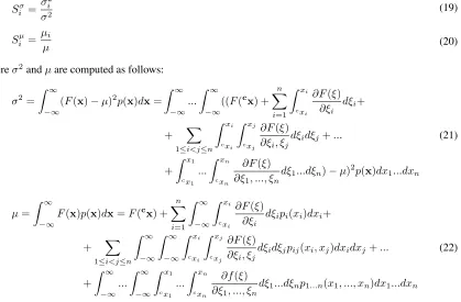
whereµirepresents the partial mean andσ2i represents the partial variance. The mean and variance sensitivity

indices for each increment function are defined as:

S_iσ= σ

2

i

σ2 (19)

S_iµ= µi

µ (20)

whereσ2_{andµare computed as follows:}

σ2=

Z ∞ −∞

(F(x)−µ)2p(x)dx=

Z ∞ −∞

...

Z ∞ −∞

((F(cx) +

n

X

i=1 Z xi

c_x i

∂F(ξ)

∂ξi dξi+

+ X

1≤i<j≤n

Z xi cxi

Z xj cxj

∂F(ξ)

∂ξi, ξjdξidξj+...

+

Z x1 c_x

1

...

Z xn c_x

n

∂F(ξ)

∂ξ1, ..., ξn

dξ1...dξn)−µ)2p(x)dx1...dxn

(21)

µ=

Z ∞ −∞

F(x)p(x)dx=F(cx) +

n

X

i=1 Z ∞

−∞ Z xi

cxi

∂F(ξ)

∂ξi dξipi(xi)dxi+

+ X

1≤i<j≤n

Z ∞ −∞

Z ∞ −∞

Z xi c_xi

Z xj c_xj

∂F(ξ)

∂ξi, ξj

dξidξjpij(xi, xj)dxidxj+...

+ Z ∞ −∞ ... Z ∞ −∞

Z x1 c_x1

...

Z xn c_xn

∂f(ξ)

∂ξ1, ..., ξn

dξ1...dξnp1...n(x1, ..., xn)dx1...dxn

(22)

wherepi(xi)is the PDF for the given variable. It should be noted that the higher order moments cannot be

computed as the superposition of the independent partial moments of the increment functions, i.e.

σ26=

2n₋₁ X

k=1

σ_k2 (23)

Kubiceket al.,4_{describe in detail the High Dimensional Model Representation and the associated Sensitivity}

Analysis theory and derivation.

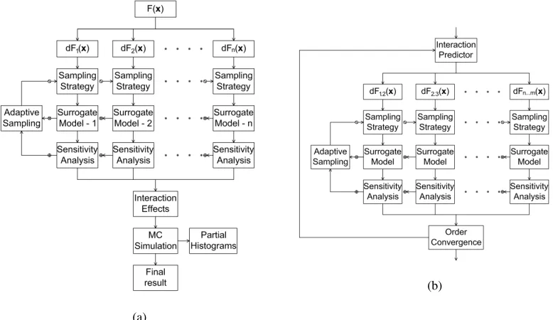
Random Input Parameter Sampling Figure 1 summarizes the methodology with a flowchart representa-tion. The function F(x) for this particular re-entry application is the time-integrated longitude and latitude at ground impact. The function F(x) is decomposed into increment functions dFn(x) as described in the

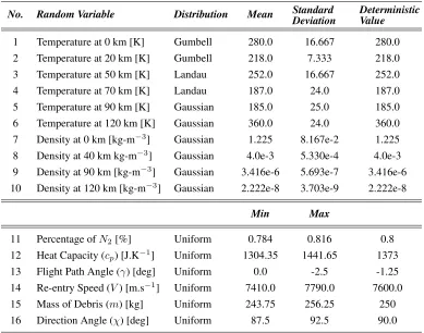
previous section, wherenis the number of considered uncertain parameters. Table 1 gives the considered uncertain parameters and the associated distribution types used for this work. For Gaussian distributions, the table provides the values for mean, standard deviation and the typical values used in a deterministic analysis. For uniform distributions, the minimum, maximum, and deterministic values are provided.

independent increment functions provides insight for predictions into relative importance of higher order interaction increment functions. Higher order increment functions with insensitive independent increment functions are predicted to have little contribution and are neglected, helping to reduce the functions calls and, therefore, the computational costs. Sensitivity analysis is then performed on the non-neglected higher order increment functions to determine the functions that can be further neglected, again saving expensive function calls towards surrogate model development. The developed surrogate models are sampled using the Monte Carlo technique to compute the statistical properties of each increment function. This allows to visualize through histograms the importance of each random variable and higher order interactions. The histograms of the independent increment functions will henceforth be also referred to as partial histograms.

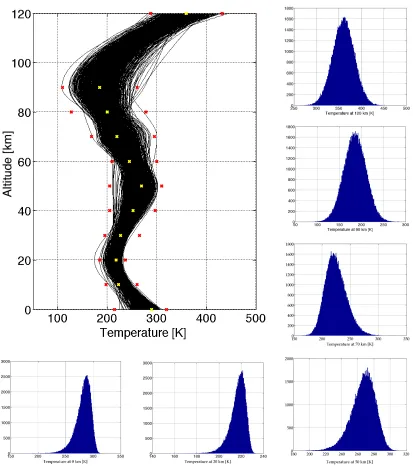
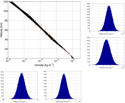
Interpolation routines were developed for atmospheric temperature and density based on the temperature and density distributions given in Table 1. The mean and standard deviations were derived from the US standard atmosphere.9 _{The data in the US standard atmosphere is provided to an altitude of about 90 km.}

The mean value at 120 km was read of the US standard atmosphere table and the standard deviation was assumed to be the same as at 90 km. Figures 2 and 3 show 1000 samples drawn from the temperature and density interpolation routines, constrained to the data points, respectively. Each function call uses one such sample. Also shown in Figures 2 and 3 are the visual representations of temperature and density distributions, respectively, for the different altitudes.9

The atmosphere is assumed to be composed of N2 and O2 and the contribution of N2 is assumed to be uncertain. The heat capacity of the free-stream air that has an effect on the computation of drag coefficient through the pressure behind the shock is also assumed to be uncertain. The flight path angle of an uncontrolled object is considered uncertain and expected to be a shallow value and play a significant role on the trajectory. The re-entry speed, mass of object and direction angle at 120 km are also considered uncertain. The central value of these parameters are based on the orbital and object characteristics. All the uncertain variables are considered as statistically independent.

RESULTS AND DISCUSSION

The output of interest for the current study is the longitudinal and lateral distribution of the impact location. This is computed using the following relation:

y=f(x)Re (24)

wheref(x)is the output of the re-entry trajectory simulation code and represents the longitude and latitude angle for longitudinal distance from the entry point and lateral distance from the entry direction, respectively, andReis the radius of the Earth.

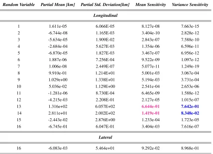
The relation in Eq. 24 is used to compute the contributions of each increment function to the longitudinal and lateral distributions, where the final distributions are computed as the sum of the contributions of the increment functions. Table 2 and Table 3 give the sensitivity indices associated with the independent and interaction increment functions, respectively. Increment functions that have a sensitivity of less than 1% are neglected. The partial means represent the offset from the deterministic values computed using the central value of the corresponding random input parameter distribution. The partial standard deviations are the contribution of the given increment function to the standard deviation of the overall distribution. The mean and variance sensitivity represent the influence of the given random parameter considering all other random parameters.

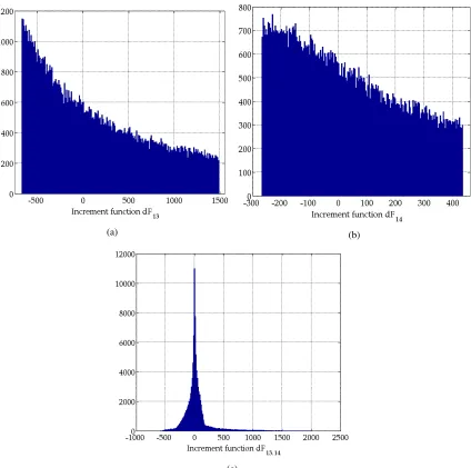
Figure 4 shows the histograms of the increment functions for the longitudinal impact distance. Figures 4a and 4b show that the flight path angle (dF13) and the re-entry speed (dF13) functions have parabolic shapes (i.e x2_{) resulting in a output that is always positive. This suggests that the same error in measuring higher} velocities will lead to a larger uncertainty. Also, the size of the contribution suggests that these two variables are responsible for the overall shape of the final distribution. Figure 4c shows the partial histogram for the interaction function of variable 13 and 14 (dF13.14).

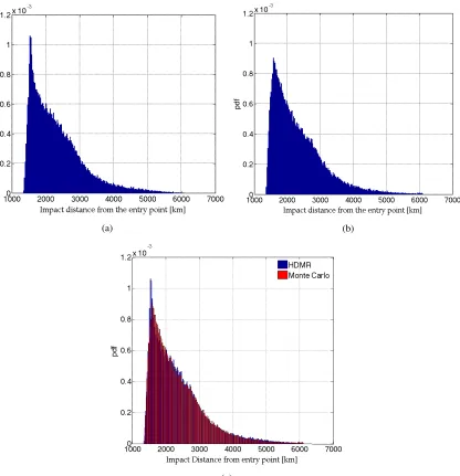
Figure 5a shows the final distribution in the longitudinal direction derived as the sum of the distributions shown in Figure 4. The final distribution has a sharp peak that smoothly transitions into a long tail. The peak is a result of the second order functions for surrogate models of (dF13) and (dF14) shown in Figures 4a and 4b, respectively. The long tail in the final distribution is a result of the surrogate model for the interaction function (dF13.14). The tail is caused by a steep ascent in the underling function in one of the corners of the given stochastic domain, i.e. to avoid such a strong tail, the input distributions need to be shortened from one side. The smooth decrease on the left side of the distribution (dF13.14) is responsible for smooth decrease on the left side in the final distribution (Figure 5a).

Results obtained with the HDMR methodology are validated using those from a Monte Carlo (MC) Anal-ysis using 1e5 samples. Figures 5b and 5c show the longitudinal distribution obtained using the MC and the overlay of the HDMR and MC distributions, respectively. As can be seen from the overlay, the peak of the MC distribution is lower than that of the HDMR with some of the MC distribution mass just to the right of the peak getting transferred to the sharp peak for the HDMR distribution. This difference is acceptable and is due to the accuracy of the underlying surrogate models set to be 1% in this work. The statistics of the two distributions are given in Table 4 and it can be seen that aside from the small difference in the peak, the distributions are simply identical.

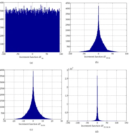
Figure 6 shows the histograms of the increment functions for the lateral impact distance. Figure 6a shows that the direction angle (dF16) surrogate model is a linear function with translation of the uniform input to output distribution. Important contribution are made by the interaction effects of (dF13.16), (dF14.16), and (dF13.14.16). Both (dF13.16) and (dF14.16) have a sharp peak around zero and smooth transitions to the tail on both sides. (dF13.14.16) exhibits a very sharp peak around zero with the distribution quickly converting to very thin but long tails on either side. The influence of the higher order interactions on the final distribution is well explained in work of.4

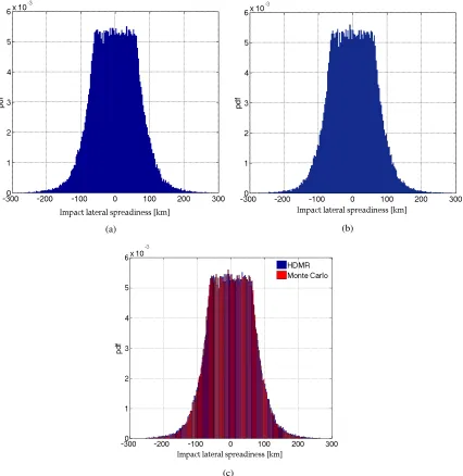
For the final lateral distribution as shown in Figure 7a, the main contribution is from the direction angle as given in Table 2. The distribution exhibits a smooth Gaussian like transition from the tails to the peak where a plateau feature is quiet clearly visible. The smooth transition is contributed by (dF13.16) and (dF14.16), whereas the plateau is derived from the uniform distribution of (dF16). The very long tails are derived from (dF13.14.16). Comparison with the MC lateral distribution shown in Figure 7b with the statistics in Table 4 and the overlay show in Figure 7c validate the HDMR methodology. Figure 8 show that comparison of the 2-Dimensional distribution use in the calculation of the total impact area. The comparison again confirms identical distributions with the interaction effects providing for 2-D spread.

In addition to the case with 16 random variables, three additional cases were simulated: 1) a case with 12 random variables accounting for uncertainty in atmospheric conditions only, 2) a case with 13 random variables accounting for uncertainty in atmospheric conditions + flight path angle (γ), and 3) a case with 15 random variables accounting for uncertainty in atmospheric conditions + flight path angle (γ) + object properties of mass and re-entry speed. These cases provide an insight into the effect of neglecting to account for uncertainties in some of the important parameters. It is obvious and expected that not considering the direction angle as uncertain and not modeling for fragmentation will collapse the lateral distribution down to the deterministic solution in that direction. Therefore, we examine the other cases on the basis of the final distribution in the longitudinal direction.

variables. Table 5 gives the number of expensive functions calls required to develop the surrogate models for the different cases. As expected, the number of function calls increases with addition of uncertain input parameters. However, in all the different cases the HDMR methodology reduces the number of expensive functions calls by more than 2 orders of magnitude. This allows the simulations to be run on a regular desktop machine and does not require expensive time on supercomputers.

Figure 9 shows the distributions for the impact distance from the entry point for the three additional cases. Figure 9a shows that accounting for only the atmospheric uncertainties results in the coveted Gaussian distri-bution spread over a little more than 100 km. Figure 9b shows that when also taking into account uncertainty in the flight path angle (γ), the distribution departs significantly from the Gaussian with the spread growing to close to 2400 km. Figure 9c shows that accounting for the uncertainty in objects properties, mainly the re-entry speed, can further influence the ground impact distribution with the spread now rising to over 4500 km. The second order velocity effects through drag as well as velocity interaction effect, as derived from the sensitivity data in Tables 2 and 3, results in a slender but elongated tail. Unlike a Gaussian distribution, the mean values of the distributions for the 13D an 15D cases are significantly offset from the peak of the distributions. For reference, the deterministic impact location in the longitudinal direction corresponding to the central values of the distributions for random input variables lies at approximately 2400 km. As can be seen, the peaks of the distributions for all the cases are significantly offset from the deterministic solution.

CONCLUSION

Current re-entry modeling tools perform the analysis in a deterministic sense and do not include any uncer-tainty treatment. This work presents progress towards incorporating unceruncer-tainty treatment into the modeling of atmospheric re-entry of space debris using a recently developed novel high-dimensional derivative based uncertainty quantification approach. Validation of the results obtained from the High Dimensional Model Representation methodology with a Monte Carlo Analysis is also presented. The work will be incorporated into the, currently under development, Free Open Source Tool for Re-entry of Asteroids and Space Debris (FOSTRAD).

Re-entry simulations with initial conditions corresponding to a circular orbit are performed for a spherical object accounting for both aleatoric and epistemic uncertainties. Uncertainties in atmospheric properties such as temperature, density, composition, heat capacity, in initial condition such as speed, flight path angle, and direction angle as well as object properties such mass are considered. Multiple cases are run to develop and understanding of the effect of the uncertain parameters on the final ground impact distribution. A total of four cases are simulated: 1) a case with 12 random variables accounting for uncertainty in atmospheric conditions only, 2) a case with 13 random variables accounting for uncertainty in atmospheric conditions + flight path angle (γ), 3) a case with 15 random variables accounting for uncertainty in atmospheric conditions + flight path angle (γ) + object properties of mass and re-entry speed, and 4) a case with all 16 random variable that also includes, in addition to those in the 15D case, the direction angle.

Accounting for only the atmospheric uncertainties results in the coveted Gaussian distribution for the impact distance in the longitudinal direction spread over a little more than 100 km. However, accounting for uncertainties in the object properties results in distributions that are significantly different from a Gaussian. Taking into account the flight path angle (case 2), the distribution spread increases to close to 2400 km which further increases to over 4500 km accounting for uncertainties in the re-entry speed at 120 km (case 3 and 4). For reference, the deterministic impact location in the longitudinal direction corresponding to the central values of the distributions for random input variables lies at 2376 km. As can seen, the peaks of the distributions for all the cases are significantly offset from the deterministic solution. The lateral distribution when taking into account the direction angle (case 4) has Gaussian-like smooth transition from the tail towards the peak where a plateau feature is observed and is spread over close to 40 km.

the variance followed by the re-entry speed (V) as well as the interaction effects between the two. The two parameters independently and through interactions make up for more than 99.5% of the variance. Uncertainty in the lateral distribution is dominated by the direction angle (χ) with close to 90% variance contribution and the rest caused by the interactions between the direction angle (χ), flight path angle (γ), and re-entry speed (V).

ACKNOWLEDGMENT

Funding for Piyush Mehta is provided by the European Commission through the Marie Curie Initial Train-ing Network (ITN) STARDUST under grant number 317185.

REFERENCES

[1] W. C. Rochelle, B. S. Kirk, and B. C. Ting,User’s Guide for Object Reentry Analysis Tool (ORSAT). NASA Lyndon B. Johnson Space Center, 1999. JSC-28742, Version 5.0, Vol. 1.

[2] G. Koppenwallner, B. Fritsche, T. Lips, and H. Klinkrad, “SCARAB A multi-disciplinary code for destruction analysis of space-craft during re-entry,” Proceeding of the 5th European Symposium on Aerothermodynamics of Space Vehicles, Cologne, Germany, Nov 2005.

[3] C. Martin, C. Brandmueller, K. Bunte,et al., “A Debris Risk Assessment Tool Supporting Mitigation Guidelines,”Proceeding of the 4th European Conference on Space Debris, ESA/ESOC, Darmstadt, Ger-many, April 2005. ESA SP-587.

[4] M. Kubicek, E. Minisci, and M. Cisternino, “High dimensional sensitivity analysis using surrogate mod-eling and High Dimensional Model Representation,”International Journal for Uncertainty Quantifica-tion, 2015. accepted.

[5] I. Newton. University of California Press.

[6] S. A. Schaaf and P. L. Chambre,High Speed Aerodynamics and Jet Propulsion, ch. Flow of Rarefied Gases, pp. 1–55. Princeton, NJ: Princeton Univ. Press, 1958.

[7] P. M. Mehta, E. Minisci, M. Vasile,et al., “An Open Source Hypersonic Aerodynamic and Aerothermo-dynamic Modeling Tool,”Proceeding of the 8th European Symposium on Aerothermodynamics of Space Vehicles, Lisbon, Portugal, March 2015.

[8] P. M. Mehta, E. Minisci, M. Vasile,et al., “Sensitivity Analysis towards Probabilistic Re-Entry Mod-eling of Spacecraft and Space Debris,”Proceeding of the AIAA Modeling and Simulation Technologies Conference, Dallas, TX, June 2015. AIAA 2015-3098.

[9] “U.S. Standard Atmosphere, 1976,” Tech. Rep. NOAA-S/T 76-1562, National Oceanic and Atmospheric Administration, Washington, DC: U.S. Government Printing Office, 1976.

Table 1: Distribution properties of random input variables.

No. Random Variable Distribution Mean Standard

Deviation

Deterministic Value

1 Temperature at 0 km [K] Gumbell 280.0 16.667 280.0

2 Temperature at 20 km [K] Gumbell 218.0 7.333 218.0

3 Temperature at 50 km [K] Landau 252.0 16.667 252.0

4 Temperature at 70 km [K] Landau 187.0 24.0 187.0

5 Temperature at 90 km [K] Gaussian 185.0 25.0 185.0

6 Temperature at 120 km [K] Gaussian 360.0 24.0 360.0

7 Density at 0 km [kg-m−3] Gaussian 1.225 8.167e-2 1.225 8 Density at 40 km kg-m−3] Gaussian 4.0e-3 5.330e-4 4.0e-3 9 Density at 90 km [kg-m−3] Gaussian 3.416e-6 5.693e-7 3.416e-6 10 Density at 120 km [kg-m−3] Gaussian 2.222e-8 3.703e-9 2.222e-8

Min Max

11 Percentage ofN2[%] Uniform 0.784 0.816 0.8

12 Heat Capacity (cp) [J.K−1] Uniform 1304.35 1441.65 1373

13 Flight Path Angle (γ) [deg] Uniform 0.0 -2.5 -1.25

14 Re-entry Speed (V) [m.s−1] Uniform 7410.0 7790.0 7600.0

15 Mass of Debris (m) [kg] Uniform 243.75 256.25 250

Table 2: Sensitivity Characteristics of Independent Increment Functions for the 16D case.

Random Variable Partial Mean [km] Partial Std. Deviation[km] Mean Sensitivity Variance Sensitivity

Longitudinal

1 1.611e-05 6.066E-05 8.127e-08 7.663e-15

2 -6.744e-08 1.165E-03 3.404e-10 2.828e-12

3 -5.634e-05 1.909E-02 2.843e-07 7.588e-10

4 -2.684e-04 5.627E-03 1.354e-06 6.596e-11

5 -6.870e-05 1.827E-03 3.467e-07 6.956e-12

6 1.887e-06 7.256E-04 9.522e-09 1.097e-12

7 1.006e-08 2.449E-07 5.077e-11 1.249e-19

8 9.910e-01 1.214E+01 5.001e-03 3.067e-04

9 1.029e+00 1.338E+01 5.194e-03 3.731e-04

10 5.036e-02 1.129E+00 2.541e-04 2.653e-06

11 -1.281e-06 8.730E-04 6.465e-09 1.588e-12

12 -4.215e-03 2.208E-01 2.127e-05 1.015e-07

13 1.316e+02 6.057E+02 6.644e-01 7.642e-01

14 2.811e+01 2.002E+02 1.419e-01 8.348e-02

15 -2.443e-02 2.876E+00 1.233e-04 1.723e-05

16 -6.745e-01 6.047E-01 3.404e-03 7.616e-07

Lateral

16 -6.083e-03 5.464e+01 9.292e-02 8.968e-01

Table 3: Sensitivity Characteristics of Random Parameter Interaction Functions for the 16D case.

Random Variable Partial Mean [km] Partial Std. Deviation [km] Mean Sensitivity Variance Sensitivity

Longitudinal

13.14 3.562e+01 2.698e+02 1.798e-01 1.516e-01

Lateral

13.16 4.680e-02 1.776e+01 6.564e-01 9.248e-02

14.16 1.127e-02 5.516e+00 1.581e-01 8.924e-03

13.14.16 5.460e-03 8.842e+00 7.657e-02 2.293e-02

Table 4: Validation statics for the HDMR compared with Monte Carlo.

Longitudinal Lateral

Mean [km] Std. Deviation [km] Mean [km] Std. Deviation [km]

HDMR 2.330e+03 7.785e+02 5.664e-02 6.495e+01

Table 5: Number of function calls for model development with HDMR.

Case 12D 13D 15D 16D

# of function Calls 57 65 84 174

(a)

(b)

(a) _(b)

(c)

(a) (b)

(c)

(a) (b)

(c)

(d)

(a) (b)

(c)

(a) (b)

(a) _(b)

(c)