City, University of London Institutional Repository
Citation:
Tsanakas, A., Wuethrich, M. V. and Černý, A. (2013). Market value margin via mean-variance hedging. ASTIN Bulletin, 43(3), pp. 301-322. doi: 10.1017/asb.2013.18This is the accepted version of the paper.
This version of the publication may differ from the final published
version.
Permanent repository link:
http://openaccess.city.ac.uk/5981/Link to published version:
http://dx.doi.org/10.1017/asb.2013.18Copyright and reuse: City Research Online aims to make research
outputs of City, University of London available to a wider audience.
Copyright and Moral Rights remain with the author(s) and/or copyright
holders. URLs from City Research Online may be freely distributed and
linked to.
City Research Online: http://openaccess.city.ac.uk/ [email protected]
Market value margin via mean-variance hedging
Andreas Tsanakas∗ Mario V. W¨uthrich† Aleˇs ˇCern´y‡
March 30, 2013
Abstract
We use mean-variance hedging in discrete time in order to value an insurance liability. The prediction of the insurance liability is decomposed into claims development results, that is, yearly deteriorations in its conditional expected values until the liability is finally settled. We assume the existence of a tradeable derivative with binary pay-off written on the claims development result and available in each development period. General valuation formulas are stated and, under additional assumptions, these valuation formulas simplify to resemble familiar regulatory cost-of-capital-based formulas. However, adoption of the mean-variance framework improves upon the regulatory approach by allowing for potential calibration to observed market prices, inclusion of other tradeable assets, and consistent extension to mul-tiple periods. Furthermore, it is shown that the hedging strategy can also lead to increased capital efficiency.
Keywords: Market value margin, mean-variance hedging, market consistent valuation, cost-of-capital, Solvency II.
1
Introduction
Market consistent valuation of insurance liabilities is a fundamental feature of new regulatory
directives, as exemplified by the Swiss Solvency Test [23] and Solvency II, see [10]. Broadly
speaking, regulatory valuation techniques distinguish between liabilities that can be replicated
in deep, liquid and transparent markets and liabilities for which this is not possible. For the
former type of liabilities, following standard financial arguments, the market values equal the
initial costs of the replicating portfolios. For the latter, the market values are postulated as
the sum of the expected present value of the liabilities and a market value margin that is set using cost-of-capital arguments. Thus, an explicit link is induced between capital assessment
and valuation for regulatory purposes.
∗Corresponding author. Cass Business School, City University London, 106 Bunhill Row, London EC1Y 8TZ,
United Kingdom; [email protected].
†ETH Zurich, RiskLab, Department of Mathematics, 8092 Zurich, Switzerland.
The application of the above regulatory principle is not straightforward. First, the
cost-of-capital rate used is a rather arbitrary, exogenously specified constant figure. Second, liabilities
cannot be readily classified as perfectly replicable or completely non-replicable. It is usually
the case that a liability can only be partly hedged and it is not entirely clear how the
regula-tory valuation approach should proceed in this case. A recent effort to reconcile cost-of-capital
principles with replication arguments is given by M¨ohr [16], who obtains Solvency II valuation
formulas as a special case. Third, given the long-term nature of many insurance liabilities,
it is not clear what a multi-period extension of cost-of-capital valuation principles should be.
Salzmann and W¨uthrich [20] and W¨uthrich and Merz [26] investigate alternative multi-period
versions of cost-of-capital valuation and show that conceptually consistent approaches can
be-come computationally very expensive.
In this paper, valuation via mean-variance hedging of liabilities in discrete time is proposed;
in particular, we use the solution in terms of sequential regression of ˇCern´y and Kallsen [3].
Mean-variance hedging identifies the self-financing trading strategy that minimizes the quadratic
deviation between the investment portfolio and the insurance liability at maturity. The general
theory of mean-variance hedging is surveyed by Schweizer [21]. For more recent developments
we refer the reader to ˇCern´y and Kallsen [2] and references therein. Insurance applications of
mean-variance hedging have been more common in life insurance where products demonstrate
a higher dependence on instruments traded in financial markets, see Thomson [24], Dahl and
Møller [5], and Delong [7]. Application to non-life insurance (see Delong and Gerrard [7]) is less
frequent due to the greater difficulty in identifying suitable tradeable instruments.
However, the development of markets in insurance-linked securities, such as cat-bonds and
weather derivatives, generates the possibility of at least partially hedging (non-life) insurance
liabilities that are exposed to specific risks, such as those arising from natural catastrophes. We
do not review the large literature on such securities and their markets here, but refer to Doherty
[9] and Cummins [4]. Indicatively we mention the progress that has been made in understanding
the statistical behavior of observed cat-bond prices (Papachristou [19]) and attempts to derive
reinsurance prices that are consistent with them (Haslip and Kaishev [12]).
Mean-variance hedging is related to other incomplete market pricing methods that have been
applied to insurance. In particular, the discrete-time risk-minimization approach of F¨ollmer and
Schweizer [11] determines locally optimal trading strategies. However, these are not necessarily
self-financing as they allow the injection of capital at fixed times. For insurance applications
of risk-minimizing hedging strategies in continuous time see Møller [17, 18]. An alternative
approach has been to derive, via indifference arguments, market-consistent versions of traditional
actuarial premium calculations rules, such as the variance and standard deviation premium
principles, see Schweizer [22].
We adopt a mean-variance hedging framework that considers a terminal liability (ultimate
decomposed into its expected value and claims development results representing yearly deteri-orations (or improvements) in the liability’s prediction using conditional expected values based
on the latest information available (Merz and W¨uthrich [14]). We then assume that the liability
can be partially replicated by a tradeable instrument that pays 1 monetary unit in each period
in the case that the claims development result exceeds a given threshold. Thus, investing in the
derivative is a form of buying protection, loosely equivalent to issuing simple 1-year bonds that
are subordinated to the insurance liabilities. In addition, we allow for the possibility of investing
in a risk-free asset and in a number of stocks. The analysis thus predicates on the assumption
that a derivative as described above can be traded or indeed (its complement) issued by the
liability holder. While buying the former will not always be a feasible option, issuing the latter
is a possibility for several insurance operators. Furthermore, the valuation formulas can be seen
as worst-case scenario valuation over the set of similar derivatives written on risks that are only
partially correlated with the liability at hand (e.g. index-triggered cat-bonds).
General valuation formulas are derived for multiple time periods, multiple tradeable assets
and general asset dynamics. Simplifying assumptions lead to more transparent and practical
formulas: if (a) asset returns have state-independent one-period Sharpe ratios, and (b) asset
returns and claims development results are uncorrelated across different time periods, the market
value of the liability is decomposed into valuations of the individual claims development results.
Each of those can be written as a weighted sum of a TVaR measure applied to the claims
development result and of CAPM-type terms corresponding to the other tradeable assets. If
it is further assumed that only the derivative is tradeable, the valuation formula becomes very
similar to multi-period cost-of-capital formulas found in Salzmann and W¨uthrich [20].
While, in their simplest form, the valuation formulas obtained bear a strong similarity to
the regulatory approach, their interpretation is different. Thus, we illustrate a potential set
of alternative assumptions on which (regulatory) valuation may be based. The benefit of this
approach is, firstly, to allow in a consistent manner the extension of liability valuation formulas
to include multiple assets, partial replication, and multiple time periods. Secondly, by making
explicit the assumptions needed to obtain simple and practically useful valuation formulas, it
becomes transparent what the price paid for such simplification is.
In Section 2 the simple single-period and single-asset case is introduced and the corresponding
valuation formulas are derived. We also show that the hedging approach used may lead to a
more efficient use of capital, which is a positive side effect of the replication strategy. In Section
3, general results for the multi-period and multi-asset case are presented and valuation formulas
are derived for specific cases. Simple numerical examples illustrate the analysis. Finally, brief
conclusions are given in Section 4.
Throughout the paper we assume that the (conditional) second moments of all random
2
Single-period and single-asset case
2.1 Preliminaries
We start with a toy model to illustrate the key ideas of the paper. A single-period is considered
with two time points t= 0 and t= 1. There is an insurance liability H≥0 that has to be met at time t = 1. At time t= 0, the insurer of H invests a total amount of v monetary units in
order to replicateHas closely as possible. All assets and liabilities are considered in discounted
units and there are two tradeable assets: a risk-free asset with price 1 at time t= 0 and payoff
1 at timet= 1 and a risky asset with priceS0 att= 0 and payoffS1 att= 1. The risky asset’s
excess return is denoted by X1 =S1/S0−1.
Capital ϑ1 is invested in the risky asset (ϑ1/S0 units are bought) at time t = 0 and the
remainder of the initial wealth v−ϑ1 is invested in the risk-free asset. This asset portfolio generates value at time 1 given by v+ϑ1X1. The optimal initial wealth V0 and investmentξ1
in the risky asset with respect to a quadratic loss function are calculated by minimizing the
quadratic deviation between the liability and the asset portfolio’s pay-off. That is,
(V0, ξ1) = arg min (v,ϑ1)
E((v+ϑ1X1−H)2 )
. (1)
SinceV0 corresponds to the initial cost of replicatingHas closely as possible w.r.t. the quadratic
loss, we will throughout this paper identifyV0 with the market consistent value of H at time 0.
Standard arguments yield the solution to optimization problem (1) which reads as
ξ1 =
Cov(X1, H) Var(X1)
, (2)
V0 = E(H)−
Cov(X1, H) Var(X1) E
(X1). (3)
In this simple setting, the value of V0 reflects the capital asset pricing model (CAPM) price of
H, where the risky asset with pay-offS1 plays the role of the market portfolio.
In the sequel, the risk measures Value-at-Risk (VaR) and Tail-Value-at-Risk (TVaR) are
used extensively. For a random variableZ with continuous distribution function and a security
levelα∈(0,1) they are defined in the common way, see for instance McNeil et al. [13],
VaRα(Z) = inf{z∈R:P(Z ≤z)≥α}, (4)
TVaRα(Z) =
1 1−α
∫ 1
α
VaRβ(Z)dβ=E(Z|Z ≥VaRα(Z)). (5)
For the latter identity to hold true we need to assume that Z has a continuous distribution
2.2 Valuation formulas
Now, a particular choice for the risky asset is made. For given random variableZ1 and threshold
d1 we define
S1=1D1 with D1 ={Z1 ≥d1}. (6)
Assume p1 =E(S1) =P(D1)∈(0,1) andS0 =q1∈(p1,1) which impliesX1=1D1/q1−1.
There are two ways of considering such pay-offs in an insurance market. First,S1 may be the
pay-off from an index-linked insurance derivative (such as a weather derivative or an industry
loss-triggered cat-bond) withZ1playing the role of the relevant index. The derivative considered
will be such that Z1 is a reasonable proxy for the liability H, hence we will require that Z1 is
positively correlated with H. In particular, the risky asset S1 pays a positive return on the
event D1 associated with a large loss in H. Probability p1 then is the real-world probability
of such an event and q1 is its risk-neutral probability implied by market prices. The condition
q1 > p1 is explained by S1 playing the role of reinsurance for large losses. While q1 ≤p1 would theoretically be possible, in practice the assumption generally holds that the cost of protection
against an adverse event is higher than its expected value, due to risk-aversion of the risk bearer.
Alternatively, consider the case that the holder of the liability H sponsors a catastrophe
bond, with D1 being the triggering event. The bond structure is such that the holder of H
pays 1 monetary unit at time 1 if D1c takes place and 0 units if D1 occurs. Let 1−q1 be the price of the bond. Then, if the sponsor issues ϑ1/q1 bonds, the gains from the trade are
−ϑ1
q1
(
1Dc
1 −(1−q1)
)
=ϑ1X1. The solution to problem (1) now gives the optimal level of debtϑ1
that should be issued. The bond will be constructed so as to maximize the correlation between
the triggerZ1 and the liabilityH. In particular, if an indemnity trigger is used, perfect positive
correlation betweenZ1 andHcan be achieved (see Papachristou [19]); otherwise so-called
basis-risk remains.
For the tradeable asset (6), equation (3) and the identity Var(S1) =p1(1−p1) yield
V0 =E(H) +
q1−p1 1−p1
[
E(H|Z1≥d1)−E(H) ]
. (7)
Formula (7) can be further refined by choosing the indemnity-based trigger Z1 = H−E(H) (the threshold d1 can now be interpreted as d1 = VaR1−p1(H)−E(H)). Assuming that H has
a continuous distribution function, formula (7) becomes
V0 =E(H) +
q1−p1 1−p1
[
TVaR1−p1(H)−E(H)
]
. (8)
Therefore valuation takes place according to a simple rule: “expected value plus a percentage
of the excess of TVaR over the expected value”.
Even when the derivative is not indemnity-triggered (i.e. H and Z1 are not perfectly
corre-lated), (8) can still be interpreted as a conservative upper bound on the value given in (7). To
but the elements of the former are comonotonic. HenceE(H1{H≥E(H)+d1})≥E(H1{Z1≥d1})
im-plies TVaR1−p1(H) ≥ E(H|Z1≥d1), where the first inequality follows from Proposition 6.2.6
in Denuit et al. [6]. With this in mind, from now on we will always identifyZ1 withH−E(H). Formula (8) bears a close resemblance to valuation formulas used under solvency regimes
such as Solvency II and the Swiss Solvency Test, where the market consistent value of a liability
is set equal to its expected value plus a risk loading deriving from a cost-of-capital charge, see
European Commission [10] and Swiss Solvency Test [23]. If the regulator prescribes a translation
invariant regulatory risk measureρto support adverse events, the market consistent value under
the cost-of-capital method equals
V0CoC=E(H) +λ[ρ(H)−E(H)], (9) whereλis thecost-of-capital rate. In Solvency II jargon, the quantityλ[ρ(H)−E(H)] is termed
market value margin.
The valuation formulas (8) and (9) are structurally similar, both satisfying the rather
prag-matic criterion of making an allowance for extreme tail events in the value of liability H via
a (tail) risk measure. However, they are derived using different economic arguments and thus
are different in significant ways. In (9) λis an exogenously given constant, while q1−p1
1−p1 in (8) is
a potentially observable and market-sensitive quantity. In (9) ρ(H) corresponds to the capital
requirement for H, while the risk measure TVaR1−p1(H) is not associated with the assets held.
In particular, for the optimal portfolio held, the investment in the risky asset would also be
reflected in the regulatory capital requirement; this is a point to which we return in Section 2.3.
Example 1. The findings of Papachristou [19], who performed statistical analysis of catastrophe
bond spreads at the time of issue, allow us to get a feeling for the potential range of the quantity
q1−p1
1−p1 . In particular, the behavior of the “multiple” is studied, that is, the ratio of the spread to
the annualized expected loss which in our simple model can be identified with the probability
p1. It is found that the multiple tends to decrease in p1, reflecting a higher risk premium for
protection against extreme events. Furthermore, it is shown how the multiple changes with time
and responds to insurance events, e.g. a rise is observed after Hurricane Katrina in 2006. For
the period of 2003-2008 studied and the sample of bonds considered, the multiple for bonds
with p1 = 1% has tended to fluctuate between about 4 and 8. This implies that the spread
rB =
E[1Dc1]
1−q1 −1 =
1−p1
1−q1−1>0 ranges from 4% to 8% and, consequently,
q1−p1
1−p1 varies from 3.8%
to 7.4%. Interestingly, the range contains the cost-of-capital rate λ= 6% favored by regulators,
see TP.5.25 in [10].
2.3 Hedging and capital efficiency
The arguments presented above focused on deriving a risk-sensitive valuation formula as an
the change in portfolio risk after investment in the derivative with pay-offS1 =1D1. This is an
issue worth considering since the buyer of such a derivative would be interested in reducing the
risk on the book and thus freeing up economic capital.
Let the solvency capital requirement be determined by a translation invariant risk measure
ρ, such that ρ(H−v) =ρ(H)−vfor allv∈Rand all random variablesH under consideration. Denote by G1 the value of the optimal investment portfolio (V0, ξ1) of (1) at time 1, i.e. G1 =
V0+ξ1X1. Then, trading in the derivative frees up capital as long as the costV0 of the trading
strategy and the capital requirement for the hedged lossH−G1 add up to less than the capital requirement for the unhedged loss H:
V0+ρ(H−G1)≤ρ(H) ⇔ ρ(H−(G1−V0))≤ρ(H). (10)
Noting that the portfolio that generates G1 has initial price V0, (10) states that investment in
the portfolio can reduce the solvency capital requirement under the risk measureρ, which looks
similar to the indifference price for G1 in an expected utility framework.
Nonetheless, it is by no means obvious that inequality (10) will generally be satisfied, since
the trading strategy is formulated to replicate the liabilityHas closely as possible in a quadratic
norm and not specifically to minimize the capital requirement described by the risk measureρ.
Some situations where (10) holds are characterized in Proposition 1 stated below.
Proposition 1. Assume H has a continuous and strictly increasing distribution function on
R+ and let the risk measure ρ be either VaRα or TVaRα at security level α ∈ (0,1). Define
k= 1−1p
1TVaR1−p1(H−E(H)). We have k >0, and inequality (10) holds if and only if
q1k≤ρ(H)−ρ(H−1D1k). (11)
In particular, the following hold:
i) Assume that VaR1−p1(H)−k >0. If α <1−p1 is small enough, such that VaRα(H) ≤
VaR1−p1(H)−k, then:
- Forρ≡VaRα, there is noq1∈(0,1)such that inequality (10) holds.
- Forρ≡TVaRα, inequality (10) holds for all q1 ∈(p1,1p−1α).
ii) If α > 1−p1 is large enough, such that VaRα(H)−VaR1−p1(H) ≥ k, then, for either
of ρ ≡ VaRα and ρ ≡ TVaRα, inequality (10) holds for all q1 ∈ (p1,1) and the freed-up
capital equals
ρ(H)−V0−ρ(H−G1) = (1−q1)k. (12)
Proof. Note that both VaR and TVaR are translation invariant and thatk >0 by the properties
of TVaR (e.g. see Property 2.4.5 in Denuit et al. [6]). We have
G1−V0=ξ1X1 =
Cov(X1, H) Var(X1)
X1 =
1D1−q1
1−p1
It follows that ρ(H−(G1 −V0)) = ρ(W) +q1k, where W = H −1D1k. Thus, the freed-up
capital can be written as ρ(H)−ρ(H −(G1 −V0)) = ρ(H)−ρ(W)−q1k, so that to satisfy
inequality (10) we need requirement (11).
Let d=d1+E(H) which impliesD1={H≥d} and VaR1−p1(H) =d. We have for w∈R
P(W ≤w) = P(W ≤w, D1) +P(W ≤w, Dc1)
= P(d≤H≤w+k) +P(H ≤min{w, d}). Continuity of the distribution function F of H and k >0 immediately imply
P(W ≤w) =
F(w), w≤d−k,
F(w+k)−F(d) +F(w), d−k < w < d,
F(w+k), d≤w.
It is easily seen that the distribution ofW is also continuous and strictly increasing. Moreover,
when VaRα(H)≤d−k (corresponding to Case i)), it is VaRα(W) = VaRα(H). On the other
hand, when VaRα(H) ≥ d+k (corresponding to Case ii)), we have P(W ≤ VaRα(H)−k) =
P(H ≤VaRα(H)) =α, such that VaRα(W) = VaRα(H)−k. We now deal with the two cases
separately.
Case i) Assume d−k >0 and choose VaRα(H)≤d−k.
1. First let ρ ≡ VaRα. Then VaRα(H−1D1k) = VaRα(W) = VaRα(H) such that condition
(11) cannot be satisfied for anyq1>0 (note thatk >0).
2. Now let ρ ≡ TVaRα. Observe that the vectors (H,1{H≥VaRα(H)}) and (H,1{W≥VaRα(W)})
have the same marginals, but the elements of the former are comonotonic. This implies inequality
E(H1{H≥VaRα(H)})≥E(H1{W≥VaRα(W)}), which follows from Proposition 6.2.6 in Denuit et al.
[6]. Consider now, using VaRα(W) = VaRα(H),
TVaRα(H)−TVaRα(W) =
1 1−α
[
E(H1{H≥VaRα(H)}))−E(W1{W≥VaRα(W)})
]
≥ 1
1−α [
E(H1{W≥VaRα(W)}))−E(W1{W≥VaRα(W)})
]
= k
1−αE(1D11{W≥VaRα(W)})
= k
1−αP(H≥max{d, k+ VaRα(H)}) = k
1−αP(H≥d) = p1 1−αk.
Hence, by (11) it is sufficient to have q1 ≤ 1p−1α for inequality (10) to hold.
Case ii) Assume VaRα(H)≥d+kwhich gives VaRα(W) = VaRα(H)−k.
1. First let ρ≡VaRα. The freed up capital equals VaRα(H)−VaRα(W)−q1k=k−q1k, which proves the stated result.
2. Now considerρ≡TVaRα. Forβ∈[α,1) monotonicity implies VaRβ(H)≥VaRα(H)≥d+k.
in (5) the freed up capital statement immediately follows from VaRβ(H)−VaRβ(W)−q1k = k−q1k.
Case i) of Proposition 1 refers to the case where the security level α is so low that the
risk reduction effected by the derivative is not reflected in the VaR measure, due to the risk
measure’s insensitivity to the extreme tail of the distribution ofH. Thus, investing any amount
in the derivative incurs a cost with no apparent benefit. When TVaR is used, the extreme
tails are reflected in the risk measurement and the benefit from investing in the derivative is
recognized, as long as the derivative is not too expensive (q1 is not too high). On the other
hand, Case ii) refers to the situation where the security level α is very high such that under all
scenarios considered by the risk measure, the derivative produces a pay-off of 1 monetary unit,
which is always higher than the priceq1 <1. Consequently, a capital saving is always produced.
However, the freed-up capital, as seen in equation (12), depends on the price q1. Thus, if q1
is close to its lowest level p1, there is no market risk premium for the derivative and the freed
up capital is maximized. On the contrary, if q1 is close to 1, the market considers the event of
the derivative paying as nearly certain, such that the derivative becomes very expensive, and
investing in it produces only a small capital reduction.
Of course, in many cases it will be −k <VaRα(H)−VaR1−p1(H)< k, a case not fully
char-acterized in Proposition 1. The following numerical example shows that for realistic parameter
choices, investment in the derivative will tend to be capital efficient.
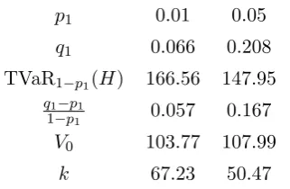
Example 2. Let H be log-normally distributed such that E(H) = 100, Var(H) = 202. We
consider two cases of the derivative, with p1 = 0.01 andp1 = 0.05. For illustrative purposes, we
follow again Papachristou [19], choosing for p1 = 0.01 (resp. p1 = 0.05) a multiple of 6 (resp.
[image:10.595.221.382.527.632.2]4), leading to q1 = 0.066 (resp. q1= 0.208).
Table 1: Valuation of a log-normal liability with E(H) = 100, Var(H) = 202.
p1 0.01 0.05
q1 0.066 0.208
TVaR1−p1(H) 166.56 147.95
q1−p1
1−p1 0.057 0.167
V0 103.77 107.99
k 67.23 50.47
Table 1 summarizes the quantities needed for the valuation of the liability H according to (8),
as well as the value k = 1−1p
1TVaR1−p1(H −E(H)) appearing in Proposition 1. While for
p1 = 0.05 the risk measure TVaR1−p1(H) is substantially lower, this is compensated by a higher
ratio q1−p1
1−p1 , such that the liability H has a higher market value V0 forp1 = 0.05.
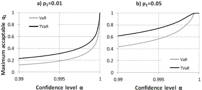
It is easy to check that for all security levelsα∈[0.99,0.999] (a plausible range for regulatory
Figure 1: Maximumq1 such that inequality (10) is satisfied.
value of the priceq1 that leads to freeing up capital is given by the relation q1 ≤ (
ρ(H)−ρ(H−
1D1k)
)
/k, whereρ≡VaRαorρ≡TVaRα. The maximum such level ofq1 is plotted in Figure 1 against the security levelα of the regulatory risk measure used, forα∈[0.99,1). It is seen that in each case the value ofq1 is well below the plotted curves, such that for the plausible range of
security levels α, investment in the derivative indeed frees up capital.
3
The multi-period and multi-asset case
3.1 Preliminaries
We extend the previous setup to a model with several assets traded over multiple time periods.
We consider a finite time horizon T ∈ N and a finite set of trading dates T = {0,1, . . . , T}. The filtered probability space is denoted by (Ω,P,F,F) with finite and discrete time filtra-tion F = (Ft)t∈T such that F0 = {∅,Ω} and F = FT. The corresponding conditional
expec-tations, variances, and covariances are denoted by Et(X) = E(X|Ft), Vart(X) = Et(X2) −
Et(X)2, Covt(X, Y) =Et(XY)−Et(X)Et(Y) fort∈ T.
The insurance liability is represented by a non-negative, FT-measurable, square-integrable
random variable H ∈L2(P). We assume that we have n ∈N tradeable risky assets with price processes represented by the n-dimensional, F-adapted stochastic process (St)t∈T. Denote the
elements of St by St(i),i= 1, . . . , n and let S
(i)
t >0. Xt is then the vector of one-period excess
returns with elements Xt(i) = St(i)/St(−i)1 −1. We assume Et(Xt(+1i) X (j)
t+1) < ∞ for all i, j and t < T, and that the returns of traded assets are linearly independent such that the matrices {
Et(Xt(+1i) X (j)
t+1) }
1≤i,j≤n have full rank. For any vector y∈R
n,y′ denotes the transpose ofy.
initial endowment v and trading strategyϑis
Gv,ϑt =v+
t
∑
k=1
ϑ′kXk. (13)
By its construction, the portfolio (13) is self-financing. Only strategies such that Gv,ϑT ∈L2(P) are admitted; for a detailed technical discussion of admissibility see ˇCern´y and Kallsen [3].
Directly extending the discussion in Section 2, the aim is to derive the optimal initial
endow-ment and trading strategy such that the quadratic deviation between the final portfolio value
Gv,ϑT and the liabilityH is minimized. In other words, we need to solve optimization problem
arg min (v,ϑ)E0
(
(Gv,ϑT −H)2). (14)
The solution to problem (14) is provided by Theorem 8.7 in ˇCern´y and Kallsen [3]:
Theorem 2. The process given by the recursion LT = 1 and for 0< t≤T
Lt−1=Et−1(Lt)−Et−1(LtXt′)
(
Et−1(LtXtXt′)
)−1
Et−1(LtXt)
is (0,1]-valued and the probability measure P∗, defined by
dP∗ dP =
T
∏
t=1 Lt
Et−1(Lt)
,
is well defined. Let E∗t−1(·) denote conditional expectations under P∗. The following processes for 0< t≤T are well defined:
a∗t =E∗t−1(Xt′) (E∗t−1(XtXt′)
)−1 ,
b∗t =a∗t E∗t−1(Xt),
Vt∗−1 =E∗t−1 (
1−a∗tXt
1−b∗t V
∗
t
)
, VT∗=H,
ξt∗ =E∗t−1((Vt∗−Vt∗−1)Xt)′
(
E∗t−1(XtXt′)
)−1 .
For initial endowment v define the trading strategyϕ(v) = (ϕt(v)t)t∈T \{0} iteratively by
ϕt(v) =ξt∗+a∗t
(
Vt∗−1−Gv,ϕt−1(v) )
.
Then, the pair (V0∗, ϕ(V0∗))solves the optimization problem (14).
The probability measure P∗ is termed the opportunity-neutral measure. The opportunity-neutral measure P∗ is not a martingale measure. Switching to P∗ is necessary in the case that asset returns are not independent in order to compensate for one-period Sharpe ratios
at a given time not being the same in all states (see ˇCern´y and Kallsen [3]). In the case
from all variables. The probability measure P∗ reduces to P if and only if the product of bt =
Et−1(Xt′) (Et−1(XtXt′))−
1E
t−1(Xt) over alltis constant (see Cern´y and Kallsen [2], Proposition
3.28). A sufficient condition for this is to require that the maximal one-period Sharpe ratio for
each time step is known at time zero, equivalently bt is F0-measurable. Independence of asset returns is a substantially stronger condition; one can for example achieve constant Sharpe ratios
in stochastic volatility models so that the returns are not i.i.d. but thebt’s remain deterministic.
Independence is a sufficient (but not necessary) condition forbothatandbtto beF0-mensurable, that is, state-independent. It also noted that the more general form of Theorem 2 is given in
terms of price increments rather than returns; we use the current form (requiring St > 0) for
practical reasons, as the dynamics of asset returns, rather than prices, are typically specified.
3.2 Valuation of an insurance liability
We work towards deriving multi-period valuation formulas, generalizing those of Section 2. First,
we decompose the FT-measurable liabilityH ∈L2(P) as
H=E0(H) +Y1+· · ·+YT with Yt=Et(H)−Et−1(H), (15) where Yt is termed the claims development result, see Merz and W¨uthrich [14]. The notion of
the claims development result is based on the understanding that insurance companies need
to close their books after every period. At time t they will book the so-called best-estimate liabilityEt(H), updating the previous predictionEt−1(H). The resulting adjustment of the best estimate produces a claims development result of Yt in period t, which may be a gain or a
loss. Essentially, Yt corresponds to the single-period risk exposure of the holder of H and the
regulator asks for a risk measure to support possible shortfalls inYtin period t. Since the time
seriesY1, . . . , YT is formed by the innovations of a martingale, its elements are uncorrelated and
have zero mean. For the rest of the paper we will assume that Yt has a continuous and strictly
increasing distribution.
For such a decomposition of the liability H, direct application of Theorem 2 gives a general
valuation formula.
Proposition 3. ForH as in (15), the optimal initial endowment of Theorem 2 becomes
V0∗ =E0(H) +
T
∑
t=1
E∗
0 ( t
∏
i=1
1−a∗iXi
1−b∗i Yt )
Proof. From Theorem 2 we have (noting that E∗t−1((1−a∗tXt)/(1−b∗t)) = 1 andVT∗=H),
VT∗−1=E∗T−1 (
1−a∗TXT
1−b∗T H )
=E0(H) +
T−1 ∑
t=1
Yt+E∗T−1 (
1−a∗TXT
1−b∗T YT )
,
VT∗−2=E∗T−2
(1−a∗
T−1XT−1 1−b∗T−1 VT−1
)
=E0(H) +
T∑−2
t=1
Yt+E∗T−2 (
1−a∗T−1XT−1 1−b∗T−1 YT−1
)
+E∗T−2 (
1−a∗T−1XT−1 1−b∗T−1
1−a∗TXT
1−b∗T YT )
.
Iterating the process yields the required result forV0∗.
Now we assume the existence of a traded insurance derivative which we identify with the
first traded risky asset. The derivative is written at each time t−1 and pays 1 unit at time t, if the claims development result Yt exceeds a given high threshold dt. Specifically,
Xt(1) = 1Dt
qt −
1, (16)
where Dt ={Yt ≥dt},Et−1(1Dt) =pt, and qt is theFt−1-measurable price at time t−1 with
pt < qt<1. In fact, much of the following analysis remains unchanged if we assume, similarly
to Section 2, that the event Dt ={Zt ≥dt}, where Zt is an (index) variable closely correlated
toYt. For the sake of simplicity, we do not pursue this route here.
Additional assumptions give rise to formulas generalizing those of Section 2.
Proposition 4. Let Xt(1) be as in (16). Assume that at and bt are state-independent and that
for any1≤i, j ≤n and0< t < t+s≤T it is
Et−1(X (i)
t X
(j)
t+sYt+s) =Et−1(X (i)
t )Et−1(X (j)
t+sYt+s), Et−1(X (i)
t Yt+s) = 0.
Then the optimal initial endowment of Theorem 2 becomes
V0=E0(H) +
T
∑
t=1
E0 (
1−atXt
1−bt
Yt
)
=E0(H)−
T
∑
t=1 a(1)t 1−btE
0 (
pt
qt
TVaR1−pt,t−1(Yt)
) − T ∑ t=1 n ∑ i=2
a(ti)Cov0(Xt(i), Yt)
1−bt
,
whereTVaR1−pt,t−1 is the risk measure calculated with respect to informationFt−1 at timet−1.
Proof. The uncorrelatedness assumption and normalization imply
ET−2 (
1−aT−1XT−1 1−bT−1
1−aTXT
1−bT
YT
)
=ET−2 (
1−aTXT
1−bT
YT
) .
The proof of the first statement then follows from Proposition 3 working backwards in time.
The second formula derives from
E0(Xt(1)Yt) =E0 (
1 qt
1DtYt
) =E0
( pt
qt
1 ptE
t−1(1DtYt)
) =E0
( pt
qt
TVaR1−pt,t−1(Yt)
The conditions of Proposition 4 correspond, loosely speaking, to the assumption that the
conditional expected performance of assets over each time period is already known at timet= 0
and that assets and liabilities are uncorrelated across time periods. Then, the market value V0
of the liabilityH equals its expected value plus a number of terms producing valuations of the
individual claims development resultsYt. Each of the latter terms can be written as a weighted
sum of the expected value of a TVaR measure applied toYtat timet−1, scaled bypt/qt, andn−1
CAPM-type terms corresponding to the other tradeable assets. Thus, the valuation formula of
Proposition 4 bears a formal similarity to commonly used multi-period cost-of-capital formulas
termed the split of total uncertainty approach in Salzmann and W¨uthrich [20] or expected risk
marginin M¨ohr [16]. At the same time, it generalizes them by including further tradeable assets via standard valuation arguments.
If we do not consider any tradeable assets except the derivatives on Yt (n = 1) a further
simplification arises. It is easily shown that at = q2 pt−qt
t+pt−2qtpt and bt =
(pt−qt)2
q2
t+pt−2qtpt. Moreover,
ifat, bt are state independent, so are pt, qt, such that a single-asset and multi-period valuation
formula, directly generalizing (8), is obtained:
V0=E0(H) +
T
∑
t=1
qt−pt
1−pt
TVaR1−pt(Yt). (17)
A comment is due relating to the uncorrelatedness assumption of Proposition 4. For simplicity,
consider the single-asset case. Then, the proposition requires Et−2 (
1{Yt−1≥dt−1}Yt
)
= 0 and
Et−2 (
1{Yt−1≥dt−1}1{Yt≥dt}Yt
)
= Et−2 (
1{Yt−1≥dt−1}
)
Et−2 (
1{Yt≥dt}Yt
)
. While the random
vari-ables Yt−1 and Yt are uncorrelated (due to the martingale property) this does not necessarily
imply that the pairs of random variables (1{Yt−1≥dt−1}, Yt) and (1{Yt−1≥dt−1},1{Yt≥dt}Yt) are also
uncorrelated. Stronger assumptions on the joint distribution of the vector (Y1, . . . , YT) are thus
required, for instance it is sufficient to assume that the martingale innovations are independent.
Two numerical examples are now presented. In Example 3, a direct application of Proposition
4 is given for the case of two assets and several time periods. In Example 4 we discuss the case
where at, bt are not state-independent. In particular, we assume a scenario where, though the
random variables Yt are independent of each other, markets take a different view such that a
high level ofYt−1 is associated with a high market priceqt for the payoff1{Yt≥dt}.
Example 3. In this example we consider a long-termFT-measurable liability H withE0(H) =
100, T = 10 years and two tradeable assets in each period. These are a derivative with price
at time t−1 of qt and pay-off at time t of 1{Yt≥dt} and a stock with price process S
(2)
t and
excess return Xt(2). We assume that the claims development results Y1, . . . , YT are mutually
independent and so are their derivative returnsX1(1), . . . , XT(1). Moreover, the pair (Yt, Xt(2)) is
defined via a bivariate log-normal model, such that
Yt= exp
(
µt+σtZt(1)
)
−exp(µt+σt2/2
)
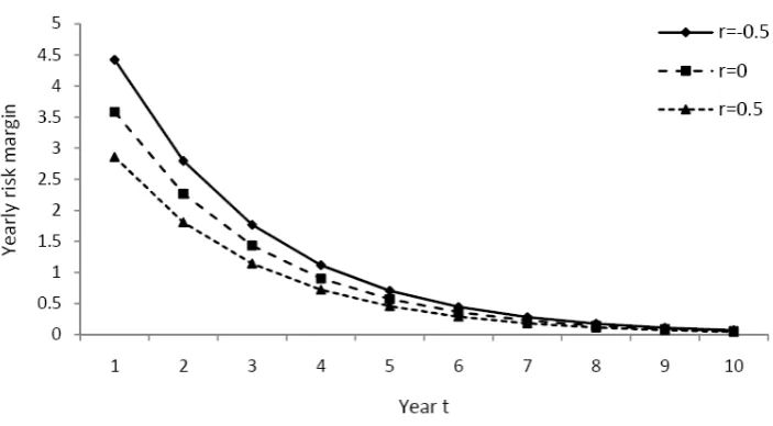
Figure 2: Yearly risk margins for different levels of correlation parameterr.
where (Zt(1), Zt(2)) follow a bivariate standard normal distribution with correlation r. This implies that we can writeZt(2)=rZt(1)+√1−r2W
t, where (Zt(1), Wt) are independent standard
normal variables. Note that, as required,Et−1(Yt) = 0. The model forYtused here is illustrative,
as in a more realistic application one would need to derive the dynamics ofYtfrom a stochastic
reserving model, see for instance Merz et al. [15].
For the derivative we use parameters pt = 0.01 and qt = 0.066 for all t, implying that the
threshold dt is always set at the 99th percentile of Yt and that the derivative price in future
periods is assumed constant. For the claims development results we useµt= 0.4586(T−t+ 1)
andσt= 0.198 for allt, such that the standard deviation ofYt reduces over time, reflecting that
uncertainty decreases with increasing information. For the stock we usem= 0.15 and s= 0.2.
Finally,ris allowed to vary in the range (−1,1). A positive (negative) correlation corresponds to
the situation when stock prices tend to increase (decrease) at times of high claims development
results (motivated by economically driven claims inflation).
We proceed by applying Proposition 4. The necessary calculations are somewhat tedious
and are documented in the Appendix. For the correlation parameter valuesr∈ {−0.5, 0, 0.5},
market values of H equaling V0(r) = {111.90, 109.64, 107.69}, respectively, are obtained. In Figure 2, we plot the market risk margin applied for each year of the liability’s run-off, that is,
the quantities ∑2i=1 a
(i)
t Cov0(Xt(i),Yt)
1−bt , t= 1, . . . , T.
We observe that the case r= 0 is equivalent to the absence of the stock such thatV0 is given
by expression (17). This means that no risk in the claims development result can be mitigated
by the asset stock price process. When r = 0.5, long positions in the stock produce a natural
hedging effect for the liability as investment returns pay for claims development results. This
r= 0. Conversely, whenr =−0.5, short positions in the stock are taken. Thus, in order to hedge the liability, negative expected stock returns are incurred. This adverse situation, analogous to
the liability being subject to systematic risk,increasesV0 in relation to the caser = 0. It can be seen from Figure 2 that the annual contributions to the market value ofH decrease with time.
This is explained by the decay of the standard deviation of Yt in our model astincreases.
Example 4. To avoid computational issues, we now consider a shorter term liability H, with
T = 2 andE0(H) = 100. In this example there is no stock correlated with claims development results such that the only tradeable asset is the derivative onY1 and Y2. Again, we assume that
the claims development results are mutually independent and
Yt= exp
(
µt+σtZt
)
−exp(µt+σt2/2
)
, t= 1,2,
where Z1, Z2 are independent standard normals. The parameters of the claims development
results areµ1 = 4.586, µ2 = 4.127, σ1 =σ2= 0.198.
We now consider a derivative with a higher probability of a pay-off than in the previous
example such thatp1 =p2 = 0.05 andq1= 0.21. However, q2 is no longer known at time t= 0,
but is instead dependent on Y1. If the derivative produces a pay-off the market price of the
derivative increases in the next period (and vice versa). Specifically, we define q2 by:
q2= {
q ≤q1, ifY1 < d1, q ≥q1, ifY1 ≥d1.
To aid comparisons, we let E0(q2) = (1−p1)q +p1q = q1. The sensitivity of q2 on past performance of the derivative is studied by considering three cases: (i) q/q = 1 giving q =q =
0.21; (ii)q/q = 2 givingq = 0.2,q= 0.4; andq/q = 4 giving q= 0.183, q= 0.730.
To calculate the market value V0∗ we use Theorem 2. In particular, we have L2 = 1 and
a∗2 =a2= E 1(X2)
E1(X22)
= p2−q2 p2+q22−2p2q2
,
b∗2 =b2 =
(E1(X2))2
E1(X22)
= (p2−q2) 2
p2+q22−2p2q2 ,
V1∗ =V1=E1 (
1−a2X2 1−b2
H )
=E0(H) +Y1+E1 (
1−a2X2 1−b2
Y2 )
=E0(H) +Y1+
q2−p2 1−p2
TVaR1−p2(Y2).
Hence V1∗ can be explicitly calculated as a function ofq2, which is in turn a function ofY1. To
deriveV0∗, we need to calculateL1 = 1−b2 and, observe thatdP∗0 =L1/E0[L1]dP0,
a∗1= E0(L1X1)
E0(L1X12)
and b∗1 = E0(L1X1) 2
E0(L1X12)E0(L1) ,
V0∗= 1
E0(L1)E0 (
L1
1−a∗1X1 1−b∗1 V
∗
1 )
These calculations of the market valueV0∗ can be easily done by Monte-Carlo simulation. Using
a simulated sample of 5·106 from Y1, we obtain that (i) for q/q = 1 it is V0∗=113.2; (ii) for
q/q = 2 it isV0∗=114.2; and forq/q = 4 it is V0∗=116.0.
Hence, with increasing sensitivity ofq2 to the outcome ofY1 the market value of the liability
increases. Intuitively, this is clear that the uncertainty is increased by increasing price sensitivity
inq2 in terms ofY1. This case may be more realistic in comparison to a scenario where derivative
prices are unaffected by observed losses, that is, where q2 does not depend on the outcome of
Y1, because investors react sensitively based on past observations. However, at least for this
short-tail example, the increase is not particularly dramatic.
3.3 Hedging and capital efficiency
In Section 2.3 the issue of capital efficiency was discussed in relation to the single-period model.
The relation between hedging and capital efficiency becomes rather convoluted in the
multi-period case. The reason for this is structural. While capital requirements in insurance are
typically calculated with respect to a 1-year time horizon, the optimal investment strategy is
formulated to minimize a quadratic error calculated at the time horizon T. In particular, the
trading strategy in each period will also reflect the performance of the portfolio to-date, which
introduces path-dependency.
Consider the simplest possible case, where Y1, . . . , YT are independent, at, bt areF0- mea-surable, and the only traded asset is the derivative on Yt. Then, from Theorem 2 it is seen that
the optimal trading strategy for initial endowmentV0 is given by
ϕt(V0) =ξt+at
(
Vt−1−GVt−0,ϕ1(V0) )
, whereξt= Et−1
((Vt−Vt−1)Xt)
Et−1(Xt2)
.
Straightforward but tedious calculations then yield ξt= CovVar0(0X(Xt,Yt)t).Hence the trading strategy
ϕt(V0) consists of two parts: ξt, the values of which in this simple setting are known at time 0,
andat(Vt−1−GtV−0,ϕ1(V0)), which reflects the value of the investment portfolio at timet. Note that ξt is essentially identical toξ1 in (2). Letδt=Vt−1−GVt−0,ϕ1(V0) represent the difference between the value of the liability and the value of the investment portfolio at time t−1. Then, since
Et−1(Xt)≤0 =⇒ at≤0, in the multi-period case we adjust the trading strategy such that, if
the shortfall is δt>0, less is invested in the risky asset and vice versa.
Analogously to what was discussed in Section 2.3, a plausible re-formulation of the capital
efficiency condition (10) at timet−1 is
ρt−1(Yt−(G V0,ϕ(V0)
t −G V0,ϕ(V0)
t−1 ))≤ρt−1(Yt), (18)
the condition that the capital required to support Yt, minus the net gains from trading over
the same interval, is less than the capital required to support Yt, assuming that all funds are
invested in the risk free asset. The left hand side of inequality (18) can be written as
ρt−1(Yt−ϕt(V0)Xt) =ρt−1(Yt−ξtXt−atδtXt). (19)
Define ˜kt=atδt+ 1−1ptTVaRt−1,1−pt(Yt).Then, retracing the first steps in the proof of
Propo-sition 1, it follows that the condition for inequality (18) to hold is, analogously to (11),
qt˜kt≤ρt−1(Yt)−ρt−1(Yt−˜kt1Dt). (20)
Finally, we remark thatξtcorresponds exactly to the investment in the stock under the
(non-self-financing) local risk-minimizing hedging strategy of F¨ollmer and Schweizer [11]. Therefore,
under such a trading strategy with explicit one-period optimization targets, the present
discus-sion of capital efficiency would be much simplified.
4
Concluding remarks
We discussed the problem of valuing insurance liabilities in discrete time through mean-variance
hedging. Key features of the proposed approach are the decomposition of the terminal liability
into claims development results and the presence of a derivative on the claims development
result in each period. In simple cases, the resulting valuation formulas become structurally very
similar to regulatory cost-of-capital based formulas. However, adoption of the mean-variance
framework improves upon such formulas, by introducing sensitivity to observed market prices,
the inclusion of other tradeable assets, and the consistent extension to multiple periods.
The similarity between the formulas derived here and the ones used in regulation should
not obscure the very different interpretations underlying them. In our approach the market
value margin obtained (difference between market consistent and expected values) does not
correspond to the cost-of-capital, but reflects the cost of a replication portfolio. Hence, it is
conceivable that a cost-of-capital loading may beadded to the market consistent value that we
obtain, since investors need to be compensated for the frictional costs that holding capital incurs
(see e.g. the discussions in Zanjani [27] and Venter [25]). The analysis of Section 2.3 shows that
the mean-variance hedging approach may also deliver a reduction in such capital costs.
It is then useful to distinguish between the possible constituent parts of the value of a
liability. Thus, if a cost-of-capital loading is added to the (partial) replication cost that our
valuation formulas reflect, this should only represent frictional capital costs. In particular, it
should not be further increased to act as a proxy for replication costs, as current regulatory
valuation approaches implicitly do. Finally, besides the cost of replication and the frictional
cost of capital, it is plausible that an additional risk load is applied via a performance measure,
VaR or TVaR; for example, mean-variance hedging approaches can be adjusted to deliver a
pre-specified minimal level of Sharpe ratio ( ˇCern´y [1], Section 13.2).
Appendix: Calculations in Example 3
For the calculations shown here it is convenient to use excess returns Xt rather than price
increments, as discussed in Section 3.1. To determine V0 we first need to calculate all terms in
at=Et−1(Xt′)Et−1(XtXt′)−1 and bt=Et−1(Xt′) Et−1(XtXt′)−1 Et−1(Xt).
Model assumption Yt= exp(µt+σtZt(1))−exp
(
µt+σ2t/2
)
provides returns
Xt(1)= 1 qt
1{Yt≥dt}−1, Xt(2)= exp(m+sZt(2))−1,
where Zt(2) =rZt(1)+√1−r2W
t and (Zt(1), Wt) are independent standard normals. Therefore,
to apply Proposition 4 we need to calculate the first and second moments of Xt as well as the
covariances Covt−1 (
Xt(i), Yt
)
fori= 1,2. The first moments ofXt are given by
Et−1 (
Xt(1))= pt qt −
1 and Et−1 (
Xt(2))= exp(m+s2/2)−1.
The second moments of Xt are given by
Et−1 (
(Xt(1))2)= 1
q2t pt(1−pt) + (
pt
qt −
1 )2
,
Et−1 (
(Xt(2))2)= 1−2 exp(m+s2/2)+ exp(2m+ 2s2),
Et−1 (
Xt(1)Xt(2))= 1−exp(m+s2/2)−pt qt
+Et−1 (
1 qt
1{Yt≥dt}exp(m+sZt(2))).
Let ˜dt = dt + exp
(
µt+σt2/2
)
= exp(µt+σtΦ−1(1−pt)
)
, where Φ is the standard normal
distribution. Then1{Yt≥dt} =1
{exp(µt+σtZt(1))≥d˜t}, such that
Et−1 (
1 qt
1{YtY≥dt}exp(m+sZ
(2)
t )
) = 1
qt
(exp(m+s2(1−r2))·g(r),
where have defined g(r) = Et−1 (
1{
Zt(1)≥(log ˜dt−µt)/σt}exp
(
srZt(1))). From the definition of ˜dt
we obtain for r = 0 the value g(0) = pt. Denote k = (log ˜dt −µt)/σt. If r > 0, we have
g(r) = exp(s2r2/2)Φ (
s2r2−srk sr
)
, using the properties of the log-normal distribution. If r < 0,
we have g(r) = exp(s2r2/2) [
1−Φ (
s2r2−srk
−sr
)] .
Finally, we move to the calculation of the covariances. They are given by
Covt−1(X (1)
t , Yt) =Et−1 (
1 qt
1{
exp(µt+σtZt(1))≥d˜t}exp
(
µt+σtZ
(1)
t
))
−pt
qt
exp(µt+σ2t/2
)
= 1 qt
exp(µt+σt2/2
) Φ
(
µt+σt2−log ˜dt
σt
)
−pt
qt
exp(µt+σt2/2
and
Covt−1(Xt(2), Yt) =Et−1 (
exp(m+µt+ (sr+σt)Zt(1)+s
√
1−r2W
t
))
−exp(m+µt+ (s2+σt2)/2
)
= exp(m+µt+ (sr+σt)2/2 +s2(1−r2)/2
)
−exp(m+µt+ (s2+σt2)/2
) .
This completes the required calculations.
References
[1] ˇCern´y, A. (2009). Mathematical Techniques in Finance. Princeton University Press.
[2] ˇCern´y, A., Kallsen, J. (2007). On the structure of general mean-variance hedging strategies. Annals of Probability 35/4, 1479-1531.
[3] ˇCern´y, A., Kallsen, J. (2009). Hedging by sequential regression revisited. Mathematical Finance 19/4, 591-617.
[4] Cummins, J. D. (2008). CAT bonds and other risk-linked securities: state of the market and recent developments. Risk Management and Insurance Review 11/1, 23-47.
[5] Dahl, M., Møller, T. (2006). Valuation and hedging of life insurance liabilities with systematic mortality risk. Insurance: Mathematics and Economics 39/2, 193-217.
[6] Denuit, M., Dhaene, J., Goovaerts., Kaas, R. (2005). Actuarial Theory for Dependent Risks: Mea-sures, Orders and Models. Wiley.
[7] Delong, L. (2012). No-good-deal, local mean-variance and ambiguity risk pricing and hedging for an insurance payment process. ASTIN Bulletin 42/1, 203-232.
[8] Delong, L., Gerrard, R. (2007). Mean-variance portfolio selection for a non-life insurance company. Mathematical Methods of Operations Research 66, 339-367.
[9] Doherty, N. A. (1997). Innovations in managing catastrophe risk. Journal of Risk and Insurance 64/4, 713-718.
[10] European Commission (2010). QIS 5 Technical Specifications, Annex to Call for Advice from CEIOPS on QIS5.
[11] F¨ollmer H., Schweizer, M. (1988). Hedging by sequential regression: an introduction to the mathe-matics of option trading. ASTIN Bulletin 18/2, 147-160.
[12] Haslip, G. G., Kaishev, V. K. (2010). Pricing of reinsurance contracts in the presence of catastrophe bonds. ASTIN Bulletin 40/1, 307-329.
[13] McNeil, A.J., Frey, R., Embrechts, P. (2005). Quantitative Risk Management: Concepts, Techniques and Tools. Princeton University Press.
[15] Merz, M., W¨uthrich, M.V., Hashorva, E. (2013). Dependence modeling in multivariate claims run-off triangles. Annals of Actuarial Science 7/1, 3-25.
[16] M¨ohr, C. (2011). Market-consistent valuation of insurance lliabilities by cost of capital. ASTIN Bulletin 41/2, 315-341.
[17] Møller, T. (1998). Risk-minimizing hedging strategies for unit-linked life insurance contracts. ASTIN Bulletin 28/1, 17-47.
[18] Møller, T. (2001). Risk-minimizing hedging strategies for insurance payment processes. Finance and Stochastics 5/4, 419-446.
[19] Papachristou, D. (2011). Statistical analysis of the spreads of catastrophe bonds at the time of issue. ASTIN Bulletin 41/1, 251-277.
[20] Salzmann, R., W¨uthrich, M.V. (2010). Cost-of-capital margin for a general insurance liability runoff. ASTIN Bulletin 40/2, 415-451.
[21] Schweizer, M. (2001). A guided tour through quadratic hedging approaches. In Jouini, E., Cvitani´c, J., Musiela, M. (eds.) Option Pricing, Interest Rates and Risk Management. Cambridge University Press, 538-574.
[22] Schweizer, M. (2001). From actuarial to financial valuation principles. Insurance: Mathematics and Economics 28/1, 31-47.
[23] Swiss Solvency Test (2006). FINMA SST Technisches Dokument, Version 2. October 2006.
[24] Thomson, R.J. (2005). The pricing of liabilities in an incomplete market using dynamic mean-variance hedging. Insurance: Mathematics and Economics 36/3, 441-455.
[25] Venter, G.G. (2004). Capital allocation survey with commentary. North American Actuarial Journal 8/2, 96-107.
[26] W¨uthrich, M.V., Merz, M. (2013). Financial Modeling, Actuarial Valuation and Solvency in Insur-ance. Springer.