Impact of VSC Converter Topology on Fault Characteristics in HVDC Transmission Systems

Impact of VSC Converter Topology on Fault Characteristics in HVDC Transmission

Systems

Dimitrios Tzelepis†, Sul Ademi †, Dimitrios Vozikis†, Adam Dy´sko†, Sankara Subramanian∗, Hengxu Ha∗

†_{University of Strathclyde, Glasgow, UK,}

dimitrios.tzelepis@strath.ac.uk, sul.ademi@strath.ac.uk, dimitrios.vozikis@strath.ac.uk a.dysko@strath.ac.uk ∗_{General Electric Grid Solutions, Stafford, UK,}

sankara.subramanian@alstom.com, hengxu.ha@alstom.com

Keywords—High voltage direct current (HVDC), DC fault-analysis, VSC converter topology, modular multi-level converter (MMC), IEC-61869, IEC-61850:9-2

Abstract

This work presents the outcome of a comprehensive study that assesses the transient behaviour of two high voltage direct current (HVDC) networks with similar structures but using different converter topologies, termed two-level and half-bridge (HB) modular multilevel converter (MMC). To quantify the impact of converter topology on DC current characteristics a detailed comparative study is undertaken in which the responses of the two HVDC network transients during dc side faults are evaluated. The behaviour of the HVDC systems during a permanent to-pole and pole-to-ground faults are analysed considering a range of fault resistances, fault positions along the line, and operational conditions as a prerequisite. Fast Fourier Transform (FFT) has been conducted analysing di/dt for both converter ar-chitecture and fault types taking into consideration sampling frequency of 96 kHz in compliance with 61869 and IEC-61850:9-2 for DC-side voltages and currents.

1. Introduction

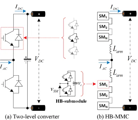
In recent years, voltage source converter high-voltage direct-current (VSC-HVDC) transmission systems have become competitive compared to systems that employ thyristor cur-rent source converters in terms of power handling capability, dc operating voltage and technology maturity [1, 2]. Such improvements have been realised employing two-level con-verters with series connected insulated gate bipolar transis-tors (IGBTs) and modular multilevel converters (MMCs), as shown in Figures 1a and 1b respectively [3, 4]. These advancements are expected to be the technology of choice for efficient grid integration. One of the main barriers for the deployment of HVDC system is the clearance of DC-side faults. Various studies have been conducted to analyse the system behaviour during DC cable faults, and a number of methods for fault location and isolation have been reported [5–7]. Fault vulnerability and high-speed protection are the major issues that constrain the development of VSC-based DC networks [8], particularly in high-power scenarios and with more than two terminals. Isolation of a faulted DC line has been proposed by utilisation of DC circuit breakers [9– 13]. However, the development of such breakers for high-voltage applications has presented a challenge for years, since unlike in AC systems, there is no natural current zero within DC systems, therefore such a breaker would have to force the current to zero and dissipate the energy stored in the system inductance [14–16]. The VSC-based transmission

systems are robust to the fault conditions on AC-side, how-ever, the most critical challenge for VSC-HVDC systems lies in its response to DC-cable faults.

Unfortunately, the two-level VSCs are defenceless against DC-side faults since their freewheeling diodes function as an uncontrolled rectifier bridge and feed the DC fault [6, 7, 17, 18], even if the semiconductor devices are turned off. Some efforts to characterise pole-to-pole and pole-to-ground faults based on VSC systems have been carried out in [5, 6, 18] and some characteristics have been established. However, further in-depth analysis into the converters behaviour is needed to improve understanding of system operation under fault conditions, and thus aid the development of effective DC protection methods.

Therefore, this paper provides detailed analysis on the be-haviour of a VSC-HVDC converter during the DC pole-to-pole and pole-to-ground faults for two-level and half-bridge submodule (HB-SM) systems in order to evaluate and understand the DC fault characteristics and their transient behaviours. The paper is organised as follows. In Section 2, a theoretical analysis of DC-side faults is carried out, both for classical two-level VSCs and HB-MMCs. Section 3 presents detailed simulation results and their analysis. Finally, Section 4, concludes the main findings.

(a) Capacitor discharge (b) Diode freewheeling (c) Grid current feeding

Figure 2: Two-level VSC cable pole-to-pole fault.

(a) IGBT Transition (b) Diode freewheeling (c) Grid current feeding

Figure 3: HB-MMC cable pole-to-pole fault.

2. HVDC Faults

2.1. Pole-to-pole faults

Such faults occur as a result of direct contact or insulation breakdown between positive and negative conductors of a DC cable. Pole-to-Pole faults are not common but can be severe to the system. A pole-to-pole fault fed from a two-level VSC can be divided into the following three stages (also illustrated in Figure 2) [6, 18].

• Stage 1.Capacitor discharge: As Figure 2a depicts, the DC-link capacitor starts discharging rapidly, con-sequently the DC voltage collapse occurs. The natural fault current response is characterised by a high peak and fast rate of change.

• Stage 2. Diode freewheeling: This stage is initiated when the DC fault commutates to the converter free-wheeling as shown in Figure 2b. This is the most hazardous period as the circulating fault current can destroy the anti-parallel diodes.

• Stage 3.Grid-side current feeding: During this stage the IGBTs are blocked and the converter behaves as an uncontrolled rectifier, injecting current into the DC side fault. The grid current contribution into fault (iGrid) is the sum of the positive three-phase fault

currents.

In an MMC a pole-to-pole fault can be also analysed in three stages. However, due to the lack of DC-link capacitor the initial response is different to the aforementioned two-level converter. The equivalent circuits representing such converter arrangement during the fault are shown in Figure 3.

• Stage 1.IGBT Transition: This is a transient occur-ring after the fault inception and before the IGBTs are turned off. The equivalent circuit during this transition is illustrated in Figure 3a.

• Stage 2.Diode freewheeling: This stage is initiated once the IGBTs are blocked. From this point the cur-rent will start passing through the diodes as indicated in Figure 3b. Concerning the arm currents at this stage, one arm current will rise while the other will be reduced to zero. The arm and cable inductance will determine the time duration of this stage.

• Stage 3.Grid-side current feeding: The fault current reaches its steady state. The equivalent circuit is shown in Figure 3c. This stage is identical to the one analysed for the two-level converter.

2.2. Pole-to-ground faults

Pole-to-pole faults are more common but at the same time they are less harmful to the system, compared to the pole-to-pole faults. In practice such faults are triggered when the insulation of the cable breaks and the live conductor touches the ground (directly or through other conducting path). During this type of faults the earthing arrangement of the system plays a significant role, as different current loops can be formed. Various earthing configurations can be achieved, and there is no specific standard, especially for MTDC netowrks [17]. Furthermore, the ground fault resis-tance cannot be ignored as its value can vary significantly, hence it is integrated into the short-circuit analysis.

Assuming a ∆/Yg transformer (with the Y winding on the

converter side) and mid-point earthed DC-link capacitors, a pole-to ground fault for a two-level converter can be analysed using the following stages:

(a) Two-level: Capacitor dis-charge

(b) Two-level: Grid current feeding (c) HB-MMC: Grid current feeding

Figure 4: Two-level and MMC cable pole-to-ground fault.

• Stage 2.Grid-side current feeding: During this stage,

even though the IGBTs are rapidly blocked, the AC-side fault current keeps feeding the fault through the converter free-wheeling diodes. This is illustrated in Figure 4b.

For MMC configuration with the same earthing arrangement of the transformer, the analysis for a pole-to-ground fault is much simpler. In fact, as a DC-link capacitor is absent, the pole-to-ground fault has only the steady state stage as illustrated in Figure 4c, which is initiated after the blocking of the IGBTs. Again, in this case the faulty-pole voltage collapses to zero, while the healthy pole voltage rises toward 2 p.u, similarly to the two-level converter.

3. Simulation-based Fault Analysis

This section includes comparative analysis of the HVDC network transients during dc faults. The simulation results are generated utilising Matlab-Simulinkr environment. The DC cable model is based on the Bergeron’s travelling wave method (also used in the Electromagnetic Transient Program (EMTP) [19]). An automatic simulation routine was devel-oped to iteratively change the fault position and resistance in order to capture the natural response of the system under a variety of fault conditions. Network parameters used for the AC grid (including transformers) and DC cable model are presented in Table 1, while the converter parameters (for two-Level and MMC) can be seen in Table 2. The fault location and ground fault resistance values used in simulation (for pole-to-pole and pole-to-ground) are included in Table 3. Distance to fault values mentioned within the paper and indicated on the result figures take as reference point the rectifier station.

The captured DC current and voltage measurements have been re-sampled at 96 kHz, with conjunction of low pass filter been applied prior to re-sampling in order to avoid any aliasing problems in compliance with 61869 and IEC-61850:9-2. Taking into account the requirements of a fast DC protection system, the rate of change of DC current (di/dt) and voltage (du/dt) have been calculated using 0.25 ms time window. All faults are triggered at t = 0.5 s and graphs are illustrated considering a 16 ms time window (including 2 ms pre-fault stage). Within the context of MTDC pro-tection, semiconductor devices (in case of MMC) were not programmed to switch off during the faults. Hence natural response of the converter has been investigated, to ensure that during the faults external DC-line protection would isolate the fault, and the VSC station would remain connected to the DC grid. Based on the analysed results presented here the emphasis is put on the current characterisation. For VSC-HVDC applications it is believed that the transient current

components are more applicable as the DC capacitors form the fundamental boundaries of the DC transmission [20, 21]. However, in order to offer a better insight into the fault response, maximum values of du/dt are also included in Table 4 (but not shown in figures due to space limitations).

Parameter Value

DC Line Resistance[RDC] 15.0 mΩ/km

DC Line Inductance[LDC] 0.96 mH/km

DC Line Capacitance[CDC] 0.012µF/km

DC Line Length 300 km

AC Voltage (L-L, RMS) 400 kV

AC Frequency 50 Hz

X/R Ratio of AC Network 10

AC Short-Circuit Level 2 GVA

Interfacing Transformer Voltages 400/330 kV

Table 1: DC Cable and AC Network Parameters

Parameter HB-MMC Two-Level VSC

DC Voltage[Vdc] ±320 kV ±320 kV

DC-Link Capacitance[Cdc] - 100µF

IGBT[Ron] 1 mΩ 1 mΩ

Arm Inductance[Larm] 2.3 mH

-Sub-module Capacitance[CSM] 50µF

-Choke Inductance[LChoke] 50 mH 60 mH

Table 2: Converter Parameters

Case Dist. [km] Sub-case Rf [Ω]

1 25 a 25

2 75 b 50

3 150 c 100

4 200 d 200

5 299 e 300

Table 3: Fault location and ground fault resistance values

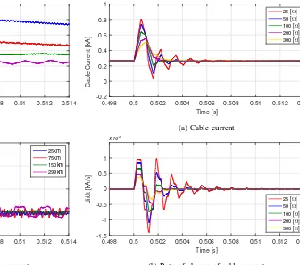
The results presented in Figures 5 to 8 which are obtained for pole-to-pole faults inject high initial currents into the cable. This is expected due to the specific structure of the MMC and lack of common DC link capacitors, thus the fault current produced by MMC is lower than the two-level. Even when the MMC’s semiconductor devices are not turned off and sub-module capacitance is included in the fault loop, the fault current is still lower due to the fact that the overall capacitance is decreased as a result of series connection of the individual capacitors.

more vulnerable. With longer distance to fault, the values of R and L included in the fault loop naturally increase. The higher values ofLincrease the rise time (by limiting the rate of change of current), while higher values ofR reduce the current peak values. The reduction of rate of change can be observed both on voltages and currents in Table 4. In case of pole-to-ground faults the fault resistance seems to have a predominant limiting effect on the fault current. However, higher fault resistance does not provide any increase of the rise time, as it does not include any additional inductance.

To better illustrate the impact of distance to fault and ground fault resistance, Table 4 includes maximum values reached for di/dt and du/dt for the two-level converter and HB-MMC. It can be observed that fault position and resistance have a limiting effect ondi/dtin all cases whiledu/dtdoes not behave in the same way. In particular, for pole-to-ground faults, the rate of change of voltage increases with distance to fault, and decreases with ground fault resistance.

In order to gain better understanding of such fault characteris-tics a Fast Fourier Transform (FFT) ofdi/dthas been carried out for both converter architectures and both types of faults. Figure 9a shows FFT analysis results for a pole-to-pole fault at 25 km. It can be seen that the majority of frequency content is located towards the lower side of the spectrum. The most striking feature of the graph is that the MMC frequency content is significantly higher than the one imposed by the two-level converter. In particular, there are distinguishable frequency components located roughly between 0.5 and 2.5 kHz. However, it can be noticed that for pole-to-pole fault the two-level converter imposes higher amplitudes in the frequency range below 1 kHz. The FFT analysis depicted in Figure 9b illustrates the frequency spectrum of a pole-to-ground fault current. In this case the MMC frequency content is observed to be higher than the two-level VSC. This is noticeable through the entire frequency spectrum. The detailed FFT based analysis (which also takes into account signal re-sampling at 96 kHz) provided the following observations :

• The frequency spectrum of interest for both types of

faults lies in the range between 0 and 3kHz.

• In case of pole-to-pole faults the two-level converter introduces higher frequency components within the range below 1kHz.

• While under the same fault condition as above the

HB-MMC imposes higher amplitudes above 1kHz, while on the contrary the two-level VSC amplitudes are practically zero beyond that frequency range.

• In case of pole-to-ground faults, the FFT analysis has indicated that HB-MMC has higher frequency components throughout the entirety of the frequency spectrum when closely compared to the two-level VSC spectrum.

4. Conclusions

Integration of high-capacity offshore renewable energy onto transmission networks is stimulating the applications of VSC-HVDC transmission networks. In this paper, pole-to-pole and pole-to-pole-to-ground fault analysis of the conventional VSC-based and MMC dc systems have been performed. Defi-nitions of the stages of the fault response are described which assist in identifying the most serious stage of a fault. Based on the fault current waveform analysis (including signal sampling frequency of 96 kHz), the following observations can be made:

Time [s]

0.498 0.5 0.502 0.504 0.506 0.508 0.51 0.512 0.514

Cable Current [kA]

-5 0 5 10 15 20 25 30

25km 75km 150km 299km

(a) Cable current

Time [s]

0.498 0.5 0.502 0.504 0.506 0.508 0.51 0.512 0.514

di/dt [kA/s]

-5 0 5 10 15

25km 75km 150km 299km x 103

(b) Rate of change of cable current

Figure 5: Two-level VSC respone for pole-to-pole fault at different locations.

Time [s]

0.498 0.5 0.502 0.504 0.506 0.508 0.51 0.512 0.514

Cable Current [kA]

-1 -0.5 0 0.5 1 1.5

25 [Ω]

50 [Ω]

100 [Ω]

200 [Ω]

300 [Ω]

(a) Cable current

Time [s]

0.498 0.5 0.502 0.504 0.506 0.508 0.51 0.512 0.514

di/dt [kA/s]

-2 -1 0 1 2

25 [Ω] 50 [Ω] 100 [Ω] 200 [Ω] 300 [Ω] x 103

(b) Rate of change of cable current

Figure 6: Two-level VSC respone for pole-to-ground fault at 25 km and different ground fault resistances.

Rf [Ω]→ 25 50 100 200 300 0 (pole-to-pole)

Dist. [km]↓ di/dt du/dt di/dt du/dt di/dt du/dt di/dt du/dt di/dt du/dt di/dt du/dt

Two-level

25 1621.2 273848.4 1222.8 238643.1 776.2 189832.5 464.9 154507.1 359.4 138813.2 12101.9 127401.9

75 1608.5 275077.4 1217.0 239450.1 766.3 190288.3 467.4 154148.0 360.6 138557.4 4430.8 74970.6

150 965.0 276617.2 837.4 240664.1 662.3 191018.2 467.0 135241.7 360 104688.3 2238.0 51890.9

200 948.2 542142.0 824.5 471739.0 653.8 374481.3 462.4 265155 357.7 205243.5 2232.1 45224.6

299 48.5 537171.0 42.2 467489.6 33.6 371185.4 23.8 262880.5 18.5 203566.6 2222.4 37801.0

HB-MMC

25 1395.9 391720.7 1090.4 380493.6 733.0 347617.5 467.7 287281.0 361.5 241537.0 8907.7 175464.0

75 1302.8 391765.0 1085.7 381001 730.3 347782.5 465.2 286281.0 360.7 240558.7 4360.4 193730.7

150 952.6 539165.1 828.6 469176.9 657.4 372480.9 465.3 293176.7 360.1 251154.5 2230.3 142741.4

200 935.5 538910.0 801.5 469180.3 656.1 372360.9 459.8 297876.2 347.6 262157.8 2228.7 129007.7

299 98.4 538250.2 85.6 468600.7 68.0 372261.6 48.4 308900.4 37.6 276947.6 2238.0 111406.0

| {z } | {z }

Pole-to-ground Pole-to-pole

Table 4: Maximum values of current and voltage derivatives in [kA/s] and [kV/s] respectively.

Time [s]

0.498 0.5 0.502 0.504 0.506 0.508 0.51 0.512 0.514

Cable Current [kA]

-5 0 5 10 15 20 25

25km 75km 150km 299km

(a) Cable current

Time [s]

0.498 0.5 0.502 0.504 0.506 0.508 0.51 0.512 0.514

di/dt [kA/s]

-5 0 5 10 15

25km 75km 150km 299km x 103

(b) Rate of change of cable current

Figure 7: HB-MMC response for pole-to-pole fault at differ-ent fault locations.

• The conventional VSC-based generates the larger DC

fault current levels, which is primarily due to the large DC-link capacitor.

• Fault current natural responses are simulated and analysed using the calculated values of di/dt and

du/dt as well as their frequency spectrum obtained using FFT. The results show that MMC-based faults have higher frequency components compared to the conventional VSC-based system throughout the entire frequency spectrum.

• Results have shown that both distance to fault and

fault resistance have a limiting effect ondi/dt.

• In the case of pole-to-ground faults, the rate of change of voltage increases with distance to fault, and decreases with higher vales of ground fault resistance.

Time [s]

0.498 0.5 0.502 0.504 0.506 0.508 0.51 0.512 0.514

Cable Current [kA]

-0.2 0 0.2 0.4 0.6 0.8 1

25 [Ω]

50 [Ω]

100 [Ω]

200 [Ω]

300 [Ω]

(a) Cable current

Time [s]

0.498 0.5 0.502 0.504 0.506 0.508 0.51 0.512 0.514

di/dt [kA/s]

-1.5 -1 -0.5 0 0.5 1

25 [Ω] 50 [Ω] 100 [Ω] 200 [Ω] 300 [Ω] x 103

(b) Rate of change of cable current

Figure 8: HB-MMC respone for pole-to-ground fault at 25 km and different ground fault resistances.

The analysis presented in this paper form a basis towards the multi-terminal protection scheme design. It has been determined that fast and selective DC line fault detection is required to make use of initial transient fault signatures. In the next step the characterisation of differences between the internal and external faults will be investigated. On-going and future work is targeting the development and demonstration of such a system.

Acknowledgements

f [kHz]

0 1 2 3 4 5 6 7 8 9 10 11 12

|Amplitude|

0 5 10 15 20 25

HB - MMC Two - level

0.5 1 1.5 2 2.5

0 2 4 6

(a) Pole-to-pole fault at 25 km

f [kHz]

0 1 2 3 4 5 6 7 8 9 10 11 12

|Amplitude|

0 5 10 15 20

HB - MMC Two - level

0 1 2 3

0 5 10 15

(b) Pole-to-ground fault at 25 km and 25Ωground fault resistance

Figure 9: FFT analysis ofdi/dtfor two-level and HB-MMC converters.

References

[1] D. V. Hertem and M. Ghandhari., “Multi-terminal VSC-HVDC for the european supergrid: Obstacles,” Renew-able and SustainRenew-able Energy Reviews, vol. 14, no. 9, pp. 3156 – 3163, 2010.

[2] D. Jovcic, D. Van Hertem, K. Linden, J.-P. Taisne, and W. Grieshaber, “Feasibility of dc transmission net-works,” in Innovative Smart Grid Technologies, 2nd IEEE PES International Conference and Exhibition on, Dec 2011.

[3] S. Cole and R. Belmans, “Transmission of bulk power,” Industrial Electronics Magazine, IEEE, vol. 3, no. 3, pp. 19–24, 2009.

[4] L. Zhang, L. Harnefors, and H.-P. Nee, “Modeling and control of VSC-HVDC links connected to island sys-tems,” Power Systems, IEEE Transactions on, vol. 26, no. 2, pp. 783–793, 2011.

[5] L. Tang and B.-T. Ooi, “Locating and isolating DC faults in multi-terminal DC systems,” Power Delivery, IEEE Transactions on, vol. 22, no. 3, pp. 1877–1884, July 2007.

[6] J. Yang, J. Fletcher, and J. O’Reilly, “Short-circuit and ground fault analyses and location in VSC-based DC network cables,”Industrial Electronics, IEEE Tran. on, vol. 59, no. 10, pp. 3827–3837, Oct 2012.

[7] J. Rafferty, L. Xu, and J. Morrow, “Analysis of volt-age source converter-based high-voltvolt-age direct current under DC line-to-earth fault,” Power Electronics, IET, vol. 8, no. 3, pp. 428–438, 2015.

[8] H. Ha and S. Subramanian, “Implementing the protec-tion and control of future dc grids,” Alstom Grid Tech-nology Centre, Innovation and TechTech-nology Department, Jan 2015.

[9] C. Greiner, T. Langeland, J. Solvik, and O. Rui, “Avail-ability evaluation of multi-terminal dc networks with dc circuit breakers,” inPowerTech, IEEE Trondheim, 2011, pp. 1–8.

[10] C. Franck, “HVDC circuit breakers: A review iden-tifying future research needs,” Power Delivery, IEEE Transactions on, vol. 26, no. 2, pp. 998–1007, April 2011.

[11] M. Callavik, A. Blomberg, J. Hafner, and B. Jacobson, “The hybrid HVDC breaker,” in ABB Grid Systems, November 2012.

[12] M. Hajian, D. Jovcic, and B. Wu, “Evaluation of semi-conductor based methods for fault isolation on high voltage dc grids,” Smart Grid, IEEE Transactions on, vol. 4, no. 2, pp. 1171–1179, June 2013.

[13] K. Sano and M. Takasaki, “A surgeless solid-state dc circuit breaker for voltage-source-converter-based hvdc systems,”Industry Applications, IEEE Transactions on, vol. 50, no. 4, pp. 2690–2699, July 2014.

[14] C. Barker and R. Whitehouse, “An alternative approach to HVDC grid protection,” inAC and DC Power Trans-mission, 10th IET International Conference on, 2012, pp. 1–6.

[15] J. Hafner and B. Jacobson, “Proactive hybrid HVDC breakers - A key innovation for reliable HVDC grids,” inCigre Symp, Sep 2011, pp. 358–361.

[16] B. Xiang, Z. Liu, Y. Geng, and S. Yanabu, “DC circuit breaker using superconductor for current limiting,” Ap-plied Superconductivity, IEEE Transactions on, vol. 25, no. 2, pp. 1–7, April 2015.

[17] J. Rafferty, L. Xu, and D. Morrow, “DC fault analysis of VSC based multi-terminal HVDC systems,” in AC and DC Power Transmission, 10th IET International Conference on, Dec 2012, pp. 1–6.

[18] S. Ademi, D. Tzelepis, A. Dysko, S. Subramanian, and H. Ha, “Fault current characterisation in VSC-based HVDC systems,” inDevelopment in Power System Pro-tection, IET Conference on, March 2016.

[19] H. Dommel, “Digital computer solution of electro-magnetic transients in single-and multiphase networks,” Power Apparatus and Systems, IEEE Transactions on, vol. PAS-88, no. 4, pp. 388–399, April 1969.

[20] G. Song, X. Cai, D. Li, S. Gao, and J. Suonan, “A novel pilot protection principle for vsc-hvdc cable lines based on fault component current,” International Journal of Electrical Power & Energy Systems, vol. 53, pp. 426– 433, December 2013.