Mass, momentum, and energy flux conservation for nonlinear wave-wave interaction

Mass, momentum, and energy flux conservation

for nonlinear wave-wave interaction

Zhen Liu,1,a),b)_{Zhiliang Lin,}1,2,b),c)_{and Longbin Tao}3,d)

1_{State Key Laboratory of Ocean Engineering, Shanghai Jiao Tong University,} 800 Dongchuan Road, Shanghai 200240, China

2_{Collaborative Innovation Center for Advanced Ship and Deep-Sea Exploration (CISSE),} Shanghai Jiao Tong University, 800 Dongchuan Road, Shanghai 200240, China 3_{School of Marine Science and Technology, Newcastle University, Armstrong Building,} Newcastle upon Tyne NE1 7RU, United Kingdom

(Received 15 July 2016; accepted 15 November 2016; published online 8 December 2016)

A fully nonlinear solution for bi-chromatic progressive waves in water of finite depth in the framework of the homotopy analysis method (HAM) is derived. The bi-chromatic wave field is assumed to be obtained by the nonlinear interaction of two monochromatic wave trains that propagate independently in the same direction before encountering. The equations for the mass, momentum, and energy fluxes based on the accurate high-order homotopy series solutions are obtained using a discrete integra-tion and a Fourier series-based fitting. The conservaintegra-tion equaintegra-tions for the mean rates of the mass, momentum, and energy fluxes before and after the interaction of the two nonlinear monochromatic wave trains are proposed to establish the relationship between the steady-state bi-chromatic wave field and the two nonlinear monochro-matic wave trains. The parametric analysis onε1andε2, representing the nonlinearity

of the bi-chromatic wave field, is performed to obtain a sufficiently small standard deviationSd, which is applied to describe the deviation from the conservation state

(Sd=0) in terms of the mean rates of the mass, momentum, and energy fluxes before

and after the interaction. It is demonstrated that very small standard deviation from the conservation state can be achieved. After the interaction, the amplitude of the primary wave with a lower circular frequency is found to decrease; while the one with a higher circular frequency is found to increase. Moreover, the highest horizontal velocity of the water particles underneath the largest wave crest, which is obtained by the nonlinear interaction between the two monochromatic waves, is found to be significantly higher than the linear superposition value of the corresponding velocity of the two monochromatic waves. The present study is helpful to enrich and deepen the understanding with insight to steady-state wave-wave interactions.Published by AIP Publishing.[http://dx.doi.org/10.1063/1.4971252]

I. INTRODUCTION

Ocean surface waves are irregular and intuitively viewed as a superposition of many mono-chromatic wave components of different frequencies and amplitudes. Nonlinear interactions among these wave components are very important to resultant wave properties. During the past several decades, a considerable number of studies have been carried out to analyze nonlinear wave interac-tion theories. Phillips1and Longuet-Higgins2initially revealed the resonant phenomenon obtained from nonlinear interactions between two or three wave trains. It was pointed out that, under specific conditions, conspicuous energy transfer occurs from primary waves to a tertiary wave, produced via

a)_{Electronic mail:liuzhen0829@sjtu.edu.cn} b)_{Z. Liu and Z. Lin contributed equally to this work.} c)_{Electronic mail:linzhiliang@sjtu.edu.cn}

d)_{Author to whom correspondence should be addressed. Electronic mail:longbin.tao@newcastle.ac.uk}

the third-order interaction. Pierson3_{derived an oscillatory third-order perturbation solution for two}

and three collinear interacting Stokes waves in deep water. However, Madsen and Fuhrman8_pointed

out that the dispersion relation obtained by Pierson3_{was not based on consistent perturbation}

prin-ciples and thus is incorrect, and they further presented a new third-order solution for bi-chromatic bi-directional water waves in finite depth, extending the second-order in finite depth and third-order in infinite depth theories of steady bi-chromatic waves. Their solution includes explicit expressions for the surface elevation, the amplitude dispersion, and the velocity potential. Dalzell4employed symbolic computation to extend the second-order wave-wave interaction theory from deep water to finite water depth. Ohyamaet al.5obtained a fourth-order solution for nonlinear interactions among multiple directional wave trains by using a Stokes-type expansion method. It was indicated that the third- and fourth-order components may produce isolated large crests in random wave fields. Chen and Zhang6 studied the interaction between a unidirectional deep-water short-wave train and an intermediate water-depth long wave using a conventional perturbation method and a phase modulation method, respectively. It was revealed that the modulation of the short-wave intrinsic frequency and potential amplitude along the long-wave surface becomes significant as water depth decreases, together with the increasing modulation of the short-wave phase, amplitude, and wave number. Zhang and Chen7_{further derived a general third-order analytical solution for the strong}

interactions among three collinear free-wave components using a perturbation method, and this solution is regarded as the kernel of third-order collinear irregular wave theory.

Most of the aforementioned studies are based on the perturbation technique due to its solid mathematical foundation on the basis of the asymptotic expansion with respect to some small parameters. As the nonlinearity increases, in order to obtain accurate results, higher-order solu-tions are required. However, the derivation of the higher-order perturbation solution for nonlinear wave-wave interaction problems can be lengthy and very complex.

Jang and Kwon9_{proposed a fixed point approach to calculate nonlinear monochromatic wave}

profiles and later Janget al.10apply to evaluate the nonlinear wave profiles of wave-wave interac-tions in a finite water depth. It is worth noting that the results by Janget al.10do not satisfy the exact kinematic and dynamic free surface boundary conditions and thus fail to capture strongly nonlinear features. To evaluate the strongly nonlinear characteristics of wave-wave interaction, Linet al.11 investigated fully nonlinear bi-chromatic unidirectional waves propagating in deep water using the so-called homotopy analysis method (HAM). The particular advantage of HAM is that it is inde-pendent of small parameters and suitable to solve strongly nonlinear problems. Other advantages associated with HAM include a greater flexibility in the selection of a proper set of base functions for the solution and a simple way in the control of the convergence rate and region of solution series.12

HAM was first applied to monochromatic, progressive waves in deep water by Liao and Che-ung.13_{Later, Taoet al.}14_{successfully extended Liao and Cheung}13_{to waters of finite depth. More}

recently, Liao15_{proposed a multiple-variable technique to investigate steady-state resonant}

progres-sive waves in deep water in the framework of HAM. It is demonstrated that there exist multiple resonant waves, and that the amplitudes of resonant wave may be much smaller than those of pri-mary waves thus the resonant waves sometimes contain fairly small part of wave energy. Xuet al.16

further confirmed the existence of steady-state resonant progressive waves in finite water depth by means of HAM and obtained qualitatively identical conclusion using the Zakharov equation. Liu and Liao17_{extended the existing results of Liao}15_{and Xuet al.}16_{on steady-state resonance from a single}

special quartet to more general and coupled resonant quartets, as well as a resonant sextet. The afore-mentioned studies on steady-state wave resonance are based on the assumption that all of the wave amplitudes, wave numbers, and wave frequencies are independent of time in the wave system. To date, however, whether or not HAM can be applied to address the unsteady-state wave resonance involv-ing complicated issues, which can account for the wave instability phenomena18(e.g., modulational instability, also known as Benjamin-Feir instability), deserves further investigation.

equations for the mean rates of the mass, momentum, and energy fluxes before and after the inter-action between collinear current-free monochromatic waves and a wave-free current based on a perturbation method. Zaman and Baddour21_{further extended the work by Baddour and Song}19,20

to a three-dimensional flow frame. However, the interaction of two nonlinear monochromatic progressive wave components which propagate independently before encountering, in terms of the conservation equations for the mass, momentum, and energy fluxes, has not been considered. In this paper, by including constant water depth in the solution procedure, the present study extends the work of Lin et al.11 from infinite water depth to finite water depth. Furthermore, based on the assumption that the steady-state bi-chromatic wave system can be obtained by the interaction of two nonlinear monochromatic progressive wave trains which propagate independently in the same direction before encountering, the present study aims to establish the relationship between the steady bi-chromatic wave field and the two nonlinear monochromatic progressive wave trains, in terms of the conservation equations for the mean rates of the mass, momentum, and energy fluxes before and after the interaction, respectively.

The present paper is organized as follows. The mathematical description of the bi-chromatic wave field is given in Sec.IIfollowing the Introduction. The definitions of the equations for the mass, momentum, and energy fluxes are introduced in Sec.III. The conservation equations for the wave-wave interaction are presented in Sec.IV. The detailed results on the parametric analysis for the standard deviation from the conservation state (Sd=0), as well as the characteristics of

the bi-chromatic wave field with sufficiently small values forSd, which is defined to describe the

deviation from the conservation state before and after interaction, are discussed in Sec.V. Finally, conclusions are given, with the detailed solution procedure based on HAM in theAppendix.

II. MATHEMATICAL DESCRIPTION OF THE BI-CHROMATIC WAVE FIELD

A. Basic equations

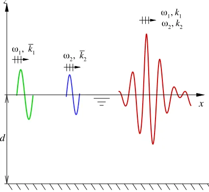
Fig.1shows the definition sketch for a steady-state bi-chromatic wave field which is assumed to be produced by the interaction of two nonlinear, monochromatic, progressive wave components that propagate independently in the same direction before interacting. A Cartesian coordinate sys-tem ₍x, z₎is adopted where the x-axis is positive in the direction of wave propagation, and the z-axis is positive vertically upwards from the still water level as shown in Fig.1. It is assumed that the nonlinear monochromatic wave train with a higher phase velocity will catch up to and interact thoroughly with the one with a lower phase velocity, yielding the steady-state bi-chromatic wave

field. For the bi-chromatic wave field, the fluid considered is inviscid and incompressible, and the flow is assumed to be irrotational. The quantities ϕ₍x,z,t₎andζ₍x,t₎are defined as the velocity potential and the wave elevation, respectively. The fluid motion described by the velocity potentialϕ is governed by the Laplace equation,

∇2ϕ₍x,z,t)=0, −∞<x<+∞, −d <z< ζ(x,t), (1)

and subject to two nonlinear free surface conditions,

∂ζ ∂t +

∂ϕ ∂x

∂ζ ∂x−

∂ϕ

∂z =0, z=ζ(x,t), (2)

gζ+1

2(∇ϕ)·(∇ϕ)+ ∂ϕ

∂t =0, z=ζ(x,t), (3)

and the following condition at the bottom:

∂ϕ

∂z =0, z=−d, (4)

where∇=₍∂/∂x, ∂/∂z₎, t denotes time, g is the gravitational acceleration, and d is the water depth. Since gravity capillary waves caused by surface tension are quite small compared to their wavelengths, the effect of surface tension is neglected.

Combining Eqs. (2) and (3), the free surface boundary condition becomes

∂2_ϕ

∂t2 +g

∂ϕ ∂z +

∂_[(∇ϕ₎·₍∇ϕ_)]

∂t +

1

2(∇ϕ)· ∇[(∇ϕ)·(∇ϕ)]=0, z=ζ(x,t). (5)

B. Multiple-variable transformation

The frequencies and wave numbers of the primary waves of the bi-chromatic wave field are defined byωiandki(i=1, 2), respectively. It is convenient to define the phase functions,

θ1=k1x−ω1t+Φ1, (6)

θ2=k2x−ω2t+Φ2, (7)

whereΦi(i=1,2)denotes an arbitrary, constant phase for zero time at the origin of thex−z

coor-dinate system. Whilstk1ω2,k2ω1, the above two variables can be applied to replace the variables

x andt, and then the timet will not appear explicitly for a steady-state wave system. Thus, the potential function and wave elevation for the steady-state bi-chromatic wave field can be expressed asϕ(x,z,t)=φ(θ1, θ2, z)andζ(x,t)=η(θ1, θ2), respectively. With these definitions, the governing

equation becomes

ˆ

∇2φ=k₁2∂

2_φ

∂θ2 1

+2k1k2

∂2_φ

∂θ1∂θ2 +k₂2∂

2_φ

∂θ2 2

+∂_∂2φ

z2 =0, −d <z< η(θ1, θ2), (8)

which is subject to the bottom boundary condition,

∂φ

∂z =0, z=−d, (9)

and the nonlinear free surface conditions,

η= 1_g(ω1

∂φ ∂θ1

+ω2

∂φ ∂θ2

− f₎, z=η₍θ1, θ2), (10)

ω2 1

∂2_φ

∂θ2 1

+2ω1ω2

∂2_φ

∂θ1∂θ2+

ω2 2

∂2_φ

∂θ2 2

+g∂φ ∂z

−2₍ω1

∂f ∂θ1

+ω2

∂f ∂θ2)

+∇ˆφ·∇ˆf =0, z=η₍θ1, θ2),

where

f =1 2



k2₁(_∂θ∂φ 1)

2_+2k 1k2

∂φ ∂θ1

∂φ ∂θ2+

k2₂(_∂θ∂φ 2)

2₊ (∂φ_∂

z)

2 

(12)

and ˆ∇=₍k1∂/∂θ1+k2∂/∂θ2, ∂/∂z). (13)

Due to the nonlinear interaction, the wave elevation should be in the form

η₍θ1, θ2)= +∞ 

m₌0 +∞ 

n=−∞

am,ncos(mθ1+nθ2), (14)

and the corresponding potential function should be in the form

φ₍θ1, θ2,z)= +∞ 

m=0 +∞ 

n=−∞

bm,nΨm,n(θ1, θ2,z), (15)

where

Ψm,n(θ1, θ2,z)=sin(mθ1+nθ2)

cosh_[|mk1+nk2| (z+d)]

cosh[|mk1+nk2|d]

, (16)

andam,n,bm,nare constants to be determined. It should be noted that (15) automatically satisfies the

governing Eq. (8) and the bottom boundary condition (9).

C. Solution procedures

As a first step to consider the nonlinear effects on the steady-state bi-chromatic waves in finite water depth, it is assumed that the nonlinear dispersion relation in the wave system can be described asωi =εi

_g

kitanh(kid) (i=1,2), whereεiis a parameter slightly larger than 1, representing the

nonlinearity of the wave system. As long asεi,ωi, anddare given,kican be easily obtained by the

nonlinear dispersion relation. Onceωi,ki, anddare known, it is not difficult to obtainam,nandbm,n

by HAM.

Linet al.11 successfully applied HAM to obtain a high-order series solution for deep-water bi-chromatic progressive waves. The effectiveness of HAM for wave-wave interaction was validated by Linet al.11by comparing the HAM solutions for the wave profile and water particle velocity with those obtained based on the perturbation technique. For the sake of simplicity, a brief description of the solution procedure in the framework of HAM is provided in theAppendix. It is worth noting that the HAM solution procedure for each nonlinear monochromatic wave train is similar to that for the bi-chromatic waves, and the detailed HAM solution procedure for monochromatic, progressive waves can also be found in the works of Liao and Cheung13_{and Taoet al.}14

D. Validation of the analytical model

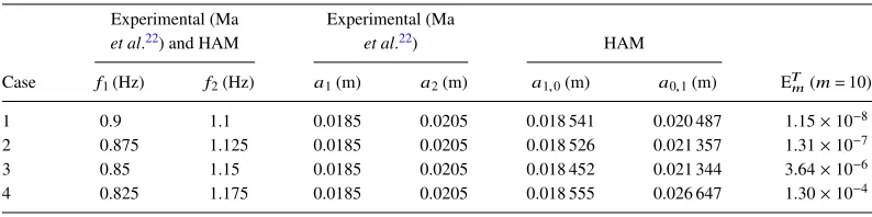
The present series solution for bi-chromatic progressive waves in finite water depth is validated by comparison to experimental data of Maet al.22_{TableIshows the parameters of the bi-chromatic}

wave cases in the experiments of Maet al.22and corresponding results obtained by HAM. As shown in TableI, for the identical frequencies (f1and f2) of primary waves of each case (cases 1-4) in the

TABLE I. Parameters of bi-chromatic waves (d=0.5 m).

Experimental (Ma

et al.22) and HAM

Experimental (Ma

et al.22) HAM

Case f1(Hz) f2(Hz) a1(m) a2(m) a1,0(m) a0,1(m) ETm(m=10)

1 0.9 1.1 0.0185 0.0205 0.018 541 0.020 487 1.15×10−8

2 0.875 1.125 0.0185 0.0205 0.018 526 0.021 357 1.31×10−7

3 0.85 1.15 0.0185 0.0205 0.018 452 0.021 344 3.64×10−6

experiments and HAM solutions, the amplitudes of primary waves (a1,0anda0,1) obtained by HAM

have slight differences with those (a1 anda2) in the experiments, respectively. This is attributed

to the nonlinear characteristics of the HAM solution. Moreover, the total averaged residual square error (ET_m) of cases 1-4 returns a fairly small value, which reaches at least the order of magnitude of 10−4. This indicates that the HAM solution for cases 1-4 possesses higher accuracy. Fig.2shows

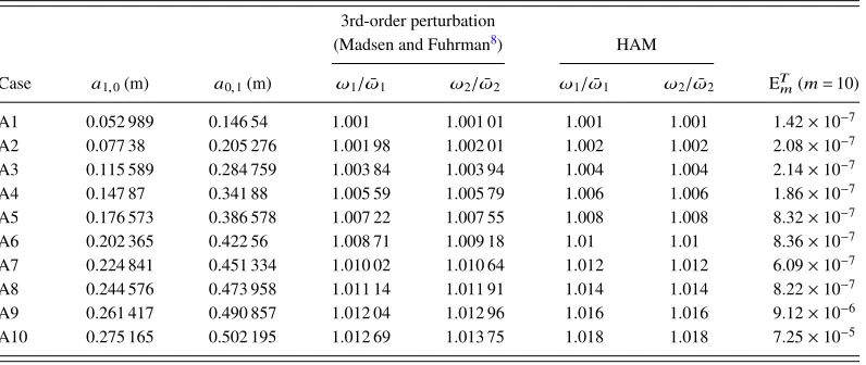
TABLE II. Parameters for the study of nonlinear amplitude dispersion (k1d=2,k2d=2.86).

3rd-order perturbation

(Madsen and Fuhrman8_{) HAM}

Case a1,0(m) a0,1(m) ω1/ω1¯ ω2/ω2¯ ω1/ω1¯ ω2/ω2¯ ETm(m=10)

A1 0.052 989 0.146 54 1.001 1.001 01 1.001 1.001 1.42×10−7

A2 0.077 38 0.205 276 1.001 98 1.002 01 1.002 1.002 2.08×10−7

A3 0.115 589 0.284 759 1.003 84 1.003 94 1.004 1.004 2.14×10−7

A4 0.147 87 0.341 88 1.005 59 1.005 79 1.006 1.006 1.86×10−7

A5 0.176 573 0.386 578 1.007 22 1.007 55 1.008 1.008 8.32×10−7

A6 0.202 365 0.422 56 1.008 71 1.009 18 1.01 1.01 8.36×10−7

A7 0.224 841 0.451 334 1.010 02 1.010 64 1.012 1.012 6.09×10−7

A8 0.244 576 0.473 958 1.011 14 1.011 91 1.014 1.014 8.22×10−7

A9 0.261 417 0.490 857 1.012 04 1.012 96 1.016 1.016 9.12×10−6

A10 0.275 165 0.502 195 1.012 69 1.013 75 1.018 1.018 7.25×10−5

the time series of wave elevation for cases 1-4 by the HAM solution, together with the experimental data by Maet al.22_{and corresponding linear superposition results. It can be clearly seen in Fig.2}

that, in comparison to the linear superposition results, the HAM solution demonstrates a much better agreement with the experimental data. This further verifies the effectiveness of the present series solution.

Linet al.11_{compared the nonlinear amplitude dispersion for bi-chromatic unidirectional waves}

in deep water obtained by HAM to the 3rd-order perturbation results by Madsen and Fuhrman.8_{It is}

demonstrated that, for the bi-chromatic waves with identical amplitude (a1,0=a0,1) of the two primary

wave components and different wave numbers(k1,k2)=(0.3,0.4), the HAM solutions agree well

with the perturbation results whenk1a1,0<0.045 (ork2a0,1<0.06) and exhibit a relatively evident

misalignment with the perturbation results when k1a1,0>0.045. In this paper, to further validate

the effectiveness of the present series solution, the nonlinear amplitude dispersions for interacting bi-chromatic unidirectional waves in finite water depth by HAM are compared to those by Mad-sen and Fuhrman.8_{TableIIshows the parameters for the study of nonlinear amplitude dispersion.}

FIG. 4. The total averaged residual square error ET

mversusmwithc0=−1 in case A10.

The wave numbers of each case of TableIIin the HAM solution and the perturbation solution are

(k1,k2)=(0.2,0.285 714). The amplitudes of primary waves (a1,0anda0,1) of each case in the HAM

solution and the perturbation solution are increasing gradually from cases A1 to A10, respectively, indicating the increasing nonlinearity of the bi-chromatic wave system. It is noted that the relative

water depths of the two primary wave components arek1d =2 andk2d=2.86, respectively,

corre-sponding to intermediate water depth conditions. As shown in TableII, the values for the relative nonlinear frequenciesω1/ω¯1andω2/ω¯2obtained by HAM agree well with the 3rd-order perturbation

results from cases A1 to A5 and have relatively large discrepancies from cases A6 to A10.

To clearly see the tendency of the nonlinear amplitude dispersion,ω1/ω¯1andω2/ω¯2are plotted

againsta1,0anda0,1in Fig.3, respectively. It can be evidently seen that the present HAM solution

appears to be different with the perturbation results starting from case A6 (a1,0=0.202 365, a0,1=

0.422 56). The total averaged residual square error for cases A6-A10 reaches at least the order of magnitude of 10−5, indicating that the present HAM solutions are highly accurate. To further demonstrate the convergence of the HAM solution, Fig.4shows the total averaged residual square error ETm versus m with c0=−1 in case A10. It can be seen that even for this rather strongly

nonlinear case (A10), ETmdecreases gradually to the order of magnitude of 10−6asmincreases from

1 to 20, a clear indication of convergence of the HAM solution for this case.

III. DEFINITION OF MASS, MOMENTUM, AND ENERGY FLUX EQUATIONS

Similar to the flux equations in Whitham,23_{the mean rates of the mass, momentum, and energy}

fluxes across a vertical section fixed in the bi-chromatic wave field, denoted byQBW_,MBW_{, andE}BW

respectively, can be written as

QBW= 1 4π2

 2π

0

 2π

0

 η

−d

ρφxdzdθ1dθ2, (17)

MBW= 1 4π2

 2π

0

 2π

0

 η

−d

(P+ρφ2x)dzdθ1dθ2, (18)

EBW= 1 4π2

 2π

0

 2π

0

 η

−d 

P+ ρ 2(φ

2 x+φ

2 z)+ρgz



φxdzdθ1dθ2, (19)

where ρdenotes density of water, and P is the total pressure which can be determined by the Bernoulli equation for the wave field as

P ρ =−

∂φ ∂t −

1 2(∇φ)

2_{−gz. (20)}

Different from the method for computing the integral quantities of the mass, momentum, and energy fluxes by means of low-order perturbation approximations by Whitham,23_{Baddour and Song,}19,20

and Zaman and Baddour,21 _{the accurate high-order homotopy series solutions for the pressure,}

water particle velocity, and free surface elevation are employed to calculate the corresponding integrations for the present bi-chromatic wave cases, i.e.,QBW_{, M}BW_{, andE}BW_{. Due to the complex}

integrands and integral upper limit incorporating the variablesxandt, it is difficult to obtain these integral quantities by direct integrating. Thus, the phase functionθi=kix−ωit(i=1,2)is applied

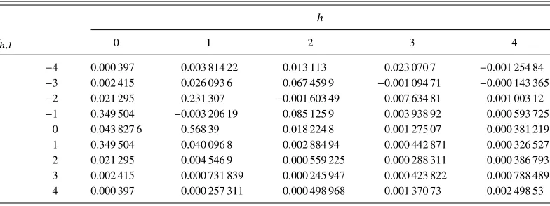
TABLE III. The coefficients for the fitted functionFQ(θ1, θ2)for the mass flux of the case BW withε1=ε2=1.008.

h

fh,l 0 1 2 3 4

l

−4 0.000 397 0.003 814 22 0.013 113 0.023 070 7 −0.001 254 84

−3 0.002 415 0.026 093 6 0.067 459 9 −0.001 094 71 −0.000 143 365

−2 0.021 295 0.231 307 −0.001 603 49 0.007 634 81 0.001 003 12

−1 0.349 504 −0.003 206 19 0.085 125 9 0.003 938 92 0.000 593 725

0 0.043 827 6 0.568 39 0.018 224 8 0.001 275 07 0.000 381 219

1 0.349 504 0.040 096 8 0.002 884 94 0.000 442 871 0.000 326 527

2 0.021 295 0.004 546 9 0.000 559 225 0.000 288 311 0.000 386 793

3 0.002 415 0.000 731 839 0.000 245 947 0.000 423 822 0.000 788 489

TABLE IV. The coefficients for the fitted functionFM(θ1, θ2)for the momentum flux of the case BW withε1=ε2=1.008.

h

fh,l 0 1 2 3 4

l

−4 0.001 678 0.016 103 2 0.053 556 8 0.084 996 3 −0.002 859 66

−3 0.010 824 0.112 297 0.261 621 −0.002 239 16 −0.005 240 12

−2 0.096 077 0.956 645 −0.003 222 21 0.057 724 7 0.004 517 14

−1 1.569 255 −0.006 635 98 0.502 256 0.021 940 7 0.002 130 71

0 1960.1 2.853 07 0.092 251 1 0.006 373 14 0.000 879 331

1 1.569 255 0.189 722 0.013 907 4 0.002 046 07 0.000 588 102

2 0.096 077 0.021 245 8 0.002 610 23 0.001 319 89 0.000 979 566

3 0.010 824 0.032 785 7 0.001 158 36 0.002 060 73 0.002 933 29

4 0.001 678 0.001 154 17 0.002 310 43 0.006 152 09 0.010 023 1

to instead ofxandtin the integrands and integral upper limit to carry out the discrete integration as illustrated below. Then, the obtained discrete integral data points are fitted using the double Fourier series. The functions obtained by fitting can be deemed as the corresponding integral expressions for the mass, momentum, and energy fluxes, respectively. The discrete integration can be described as

QDBW_i,j =  ηi,j

−d

ρφx(θ1, θ2,z)|θ1=i∆θ1,θ2=j∆θ2dz, (21)

M DBW_i,j =  ηi,j

−d [

P₍θ1, θ2,z)+ρφ2x(θ1, θ2,z)]

θ1=i∆θ1,θ2=j∆θ2dz, (22)

E DBW_i,j =  ηi,j

−d 

P(θ1, θ2,z)+

ρ 2[φx

2

(θ1, θ2,z)+φz2(θ1, θ2,z)]+ρgz 

φx

×₍θ1, θ2, z)

θ1=i∆θ1,θ2=j∆θ2

dz, (23)

where ηi,j=η(θ1, θ2)

θ1=i∆θ1,θ2=j∆θ2,i=0,1, . . . ,I, j=0,1, . . . ,J,I andJ are the numbers of the discrete points,∆θ₁=4π/Iand∆θ₂=4π/J. In the present work, the discrete integrations are calcu-lated withI=J=20 to obtain sufficient integral data points for the subsequent fitting. It is worth noting that all the integral quantity expressions for each nonlinear monochromatic wave field based on the HAM solution are similar to those for the bi-chromatic wave field.

To illustrate the calculation and fitting procedure for the discrete integration, consider the bi-chromatic wave case withε1=ε2=1.008. As shown in Figs.5(a)–5(c), the filled circles

repre-senting the integral values are obtained by using the above discrete integration. The double Fourier

seriesF₍θ1, θ2)= N 

h=0 N 

l=−N

fh,l cos(hθ1+lθ2)is employed to fit the discrete integral data points to

TABLE V. The coefficients for the fitted functionFE(θ1, θ2)for the energy flux of the case BW withε1=ε2=1.008.

h

fh,l 0 1 2 3 4

l

−4 0.005 637 0.047 375 9 0.115 674 0.031 751 2 0.031 869

−3 0.032 586 0.247 497 0.067 681 6 0.094 859 1 0.009 476 49

−2 0.218 464 0.125 411 0.276 86 0.029 396 3 0.010 873 3

−1 0.087 544 0.682 447 0.077 110 8 0.056 714 9 0.006 188 63

0 0.477 811 0.150 311 0.230 699 0.019 821 4 0.002 410 05

1 0.087 544 0.450 797 0.044 313 7 0.006 068 73 0.001 389 97

2 0.218 464 0.065 846 4 0.008 976 34 0.003 447 2 0.002 519 18

3 0.032 586 0.011 207 6 0.003 794 49 0.005 575 12 0.007 649 64

TABLE VI. The monochromatic wave parameters (d=20 m).

Case ε

Circular frequency (rad/s)

Wave number (rad/m)

Wavelength (m)

Phase velocity (m/s)

Amplitude of primary waves (m)

W1 1.002 1.983 86 0.4 15.708 4.96 0.157 823

W2 1.002 2.218 02 0.5 12.5664 4.44 0.126 214

obtain the continuous functions for the mass, momentum, and energy fluxes, which are represented by FQ(θ1, θ2), FM(θ1, θ2), and FE(θ1, θ2), respectively. Taking N =4, the Fourier coefficients fh,l

for the fitted functions for the mass, momentum, and energy fluxes of the bi-chromatic wave case withε1=ε2=1.008 were obtained, and shown in TablesIII–V, respectively. As clearly shown in

Figs.5(a)–5(c), the curves for the fitted functions agree well with the discrete integral value points, indicating that the corresponding integral quantities can be represented by the fitted functions based on the double Fourier series. Thus, the mean rates of the mass, momentum, and energy fluxes across a vertical section fixed in the bi-chromatic wave field can be obtained as

QBW_F = 1 4π2

 2π

0

 2π

0

FQ(θ1, θ2)dθ1dθ2, (24)

M_FBW= 1 4π2

 2π

0

 2π

0

FM(θ1, θ2)dθ1dθ2, (25)

E_FBW= 1 4π2

 2π

0

 2π

0

FE(θ1, θ2)dθ1dθ2. (26)

IV. CONSERVATION EQUATIONS

Baddour and Song19,20 _{proposed the conservation equations based on linear and the}

second-order perturbation solutions in terms of the mean rates of the mass, momentum, and energy fluxes of a 2D current-free wave field, a wave-free uniform current field, and a coexisting wave-current field. In their work, the wavelength, wave height, current velocity, and water depth in the combined wave-current field were obtained based on the conservation equations for the mean rates of the mass, momentum, and energy fluxes. Zaman and Baddour21_{further extended the work of Baddour}

and Song19,20to a 3D wave-current field in the framework of linear wave theory.

Without loss of generality, consider two 2D, weakly nonlinear, monochromatic wave trains propagating independently in the same direction before encountering. TableVIpresents the param-eters of the two nonlinear monochromatic wave trains, i.e., cases W1 and W2, respectively, where ε=ωi/



g_k¯_itanh(k¯_{id);ωiand ¯ki(i=1,2)are the circular frequency and wave number of the} cor-responding monochromatic waves, respectively, as shown in Fig.1. It is worth noting that the two

FIG. 7. The comparison of the discrete integral value points and fitted function curves for (a) and (d): mass flux; (b) and (e): momentum flux; (c) and (f): energy flux of cases W1 and W2.

monochromatic wave cases in the paper are indeed weakly nonlinear. This is due to the assumption that the bi-chromatic wave system is obtained by the nonlinear interaction of the two monochro-matic wave trains with wave frequencies and water depth unchanged. However, the interaction of these two weakly nonlinear monochromatic wave cases leads to a sufficiently strong nonlinear bi-chromatic wave system at a higher conservation level of mass, momentum, and energy fluxes, as discussed in the following. In fact, Liao and Cheung13_{and Taoet al.}14_{presented accurate HAM}

TABLE VII. The mean rates of the mass, momentum, and energy fluxes of cases W1 and W2.

Case Mass flux (kg/s)

Momentum flux (kg m/s2)

Energy flux (kg m2/s3) W1 0.024 682 9×103 _1960.06×103 _{0.304 792×10}3

W2 0.017 649 1×103 _1960.04×103 _{0.174 348×10}3

(0.142 tanhkd). All the HAM solutions for cases W1 and W2 are obtained with a total averaged residual error at least 10−6_{, which is defined in theAppendixand used to describe the accuracy of}

the homotopy series solution. Fig.6shows the wave profiles for cases W1 and W2 att=0. Fig.7

shows the comparison of the discrete integral value points and the fitted function curves for the mass, momentum, and energy fluxes for cases W1 and W2, respectively. It is clearly seen that the curves for the fitted functions agree well with the corresponding discrete integral value points. By means of the obtained fitted functions, the mean rates of the mass, momentum, and energy fluxes across a fixed section, which are denoted byQW_F1,M_FW1, andE_FW1for case W1 and byQW_F2,M_FW2, and EW_F2for case W2, respectively, are calculated and presented in Table VII. The conservation equations for wave-wave interaction can be summarized as

QW_F1+QW_F2=QBW_F , (27)

M_FW1+M_FW2=M_FBW, (28)

EW_F1+EW_F2=EBW_F . (29)

It is noted that the approximate solutions for the conservation equations of the mass, mo-mentum, and energy fluxes were obtained by Baddour and Song19,20 _{based on the low-order}

perturbation solutions for the current-free wave field and combined wave-current field. Due to the nonlinear feature of the interaction process, it is difficult to obtain the exact solutions for the bi-chromatic wave field, which is obtained via the interaction of the two nonlinear monochro-matic wave trains, by solving the conservation Eqs. (27)–(29). Thus, in this study, the standard deviation

Sd= 

(rQ−1)2+(rM−1)2+(rE−1)2

3 (30)

is defined to illustrate the deviation from the conservation state (Sd=0) of the mean rates of the

mass, momentum, and energy fluxes before and after the interaction of the two nonlinear monochro-matic wave trains, where

rQ=

QBW_F

QW_F1+QW_F2, rM=

M_FBW

M_FW1+M_FW2, rE =

EBW_F

EW_F1+EW_F2. (31)

Using the standard deviationSd, it is not difficult to obtain a state evaluating the deviation from the

conservation state after the interaction of the two monochromatic wave trains.

V. RESULTS AND DISCUSSION

A. Analyses based onε1=ε2

TABLE VIII. The bi-chromatic wave parameters in the case ofε1=ε2(d=20 m).

ε1 ε2 ω1(rad/s) ω2(rad/s) Sd L1(m) L2(m) a1,0(m) a0,1(m)

1.001 1.001 1.983 86 2.218 02 0.682 15.6766 12.5413 0.048 790 1 0.066 015 9

1.002 1.002 1.983 86 2.218 02 0.555 15.7079 12.5664 0.067 862 3 0.091 826 2

1.003 1.003 1.983 86 2.218 02 0.436 15.7393 12.5915 0.081 416 2 0.110 22

1.004 1.004 1.983 86 2.218 02 0.327 15.7707 12.6166 0.091 717 5 0.124 255

1.005 1.005 1.983 86 2.218 02 0.229 15.8021 12.6417 0.099 640 3 0.135 117

1.006 1.006 1.983 86 2.218 02 0.140 15.8336 12.6669 0.105 687 0.143 485

1.007 1.007 1.983 86 2.218 02 0.061 15.8651 12.6921 0.110 286 0.149 906

1.008 1.008 1.983 86 2.218 02 0.013 15.8966 12.7173 0.113 925 0.154 952

1.009 1.009 1.983 86 2.218 02 0.082 15.9282 12.7426 0.117 177 0.159 348

1.01 1.01 1.983 86 2.218 02 0.157 15.9598 12.7679 0.120 801 0.164 024

a set of ε1(=ε2)for the bi-chromatic wave field is utilized to investigate the deviation from the

conservation state by means of the standard deviationSd. TableVIIIshows the bi-chromatic wave

parameters for the conservation study. For the bi-chromatic wave field, for simplicity, it is easy to assume thatε1=ε2with the same value (1.002) as that of the nonlinear monochromatic wave

fields. As shown in TableVIII, forε1=ε2=1.002,Sd=0.555 can be obtained based on the HAM

solutions. However, forε1=ε2=1.001,Sd tends to approach a much higher value (0.682). This

indicates that a smaller value forε1(=ε2)leads to a larger discrepancy between the mean rates of the

mass, momentum, and energy fluxes before and after the interaction. Forε1(=ε2)from 1.003 to 1.01

with an increment of 0.001,Sd approaches a relatively smaller value (0.013) at ε1=ε2=1.008,

indicating that the case (ε1=ε2=1.008) is much closer to the conservation state of the mass,

momentum, and energy fluxes than other cases in TableVIII.

Fig.8shows the wave profile comparison for the cases BW withε1=ε2=1.006, 1.008, and

1.01 att=0. It can be clearly seen that the largest wave crest atx=0 becomes higher and higher asε1(=ε2)increases, whilst the largest wave trough next tox=0 becomes lower and lower. This

means that the largest wave height in the wave profile tends to increase notably asε1 increases,

although the increment in ε1 is very small. However, the profiles of the wave crest and trough

aroundx=30 m appear to be invariant.

To investigate the frequency content of the bi-chromatic wave system, the time series of the wave elevation obtained from the HAM solutions are analyzed by FFT. Figs. 9(a)–9(c) show the amplitude spectra of the bi-chromatic wave system with ε1=ε2=1.006, 1.008, and 1.01.

As shown in Figs. 9(a)–9(c), two dominant large amplitudes (at f1≈0.314 367 Hz and f2≈

0.352 342 Hz) can be clearly seen and high-order nonlinear components of each bi-chromatic wave case are rather prominent. As ε1(=ε2) increases from 1.006 to 1.01, the nonlinearity becomes

stronger and stronger and some higher-order wave components, e.g., the third order (3f1,3f2, etc.),

become increasingly significant. TableIXpresents the amplitudes of the wave components from the

FIG. 9. Amplitude spectra for the cases BW withε1=ε2=1.006, 1.008, and 1.01.

first order to the third order of the cases BW withε1=ε2=1.006, 1.008, and 1.01, respectively.

It can be clearly observed that the amplitudes of the wave components from the first order to the third order between these cases have remarkable difference. For example, the value fora(f1)in the

case ofε1=ε2=1.008 (Sd=0.013) is 0.113 925 m which is 7.5% greater than 0.105 687 m in

the case ofε1=ε2=1.006 (Sd=0.140), and 6.1% less than 0.120 801 m in the case ofε1=ε2=

1.01 (Sd=0.157). In fact, these different amplitudes indeed lead to the difference of the mean rates

of the mass, momentum, and energy fluxes between these three cases, which can be assessed by the standard deviation (Sd) values from the conservation state.

B. Analyses based onε1,ε2

As shown in TableVIII, it can be seen thatSdapproaches a relatively smaller value (0.013) in

TABLE IX. Amplitudes of the wave components from the first order to the third order of the cases BW withε1=ε2=1.006, 1.008, 1.01;ε1=1.007, ε2=1.008 andε1=1.0065, ε2=1.008.

ε1(=ε2)

Amplitude (m) 1.006 1.008 1.01 ε1=1.007, ε2=1.008 ε1=1.0065, ε2=1.008

a(f1) 0.105 687 0.113 925 0.120 801 0.129 123 0.138 147

a(f2) 0.143 485 0.154 952 0.164 024 0.144 214 0.137 890

a(2f1) 0.002 907 0.003 627 0.003 950 0.004 442 0.004 922

a(2f2) 0.007 326 0.009 165 0.009 710 0.008 641 0.008 029

a(f1+f2) 0.007 133 0.008 508 0.009 574 0.008 875 0.009 034

a(f1−f2) 0.001 206 0.001 675 0.002 460 0.001 493 0.001 472

a(3f1) 0.000 139 0.000 212 0.000 263 0.000 284 0.000 319

a(3f2) 0.000 738 0.001 256 0.001 849 0.000 974 0.000 876

a(2f1+f2) 0.000 432 0.000 604 0.000 753 0.000 668 0.000 710

a(f1+2f2) 0.000 718 0.000 992 0.001 171 0.000 985 0.000 965

a(2f1−f2) 0.009 398 0.013 054 0.012 437 0.015 433 0.016 353

a(f1−2f2) 0.038 920 0.054 585 0.060 127 0.048 538 0.043 462

conservation state (Sd=0) of the mean rates of the mass, momentum, and energy fluxes before and

after the interaction than other cases in TableVIII. Obviously, the above analysis is based on the assumption thatε1is equal toε2for the steady-state bi-chromatic wave field after the interaction.

However, it is essential to considerε1,ε2 for the bi-chromatic wave field. TableXpresents the

values forSdfor the matrix ofε1andε2ranging from 1.005 to 1.01 with an increment of 0.001. As

shown in TableX, the minimum values forSdin each row (0.02,0.010,0.009,0.013,0.027,0.034)

arises in the same column in whichε2=1.008. For the column withε2=1.008, it is noted that the

minimum value forSdis 0.009 which is calculated in the case ofε1=1.007 andε2=1.008. This

indicates thatε1,ε2can yield a lower value forSdcompared to the cases in TableVIIIwhich are

based on the assumption thatε1=ε2, e.g., there is a slight difference (0.004) forSdin the case of

ε1=ε2=1.008 andε1=1.007, ε2=1.008. It is worth noting that all the values forSdpresented in

TableXare calculated based on the HAM solutions with a total averaged residual error at least 10−6 for each steady wave field.

TableXIfurther presents the values forSdfor the matrix ofε1andε2aroundε1=1.007 and

ε2=1.008 with a smaller increment of 0.0005. As shown in TableXI, similar to the tendency in

TableX, the minimum values forSdin each row arise in the column withε2=1.008. It is clear that

compared to the case ofε1=1.007 andε2=1.008, a smaller value (0.007) forSdcan be obtained

whenε1=1.0065 andε2=1.008. This indicates that it is possible to obtain much smaller values

forSdby subdividing aroundε1=1.007 andε2=1.008 with a smaller increment. However, in this

paper, the case BW withε1=1.0065,ε2=1.008, andSd=0.007 is supposed to be highly close to

the conservation state, thus it is not essential to seek smaller values forSd.

TABLE X. The standard deviationSdfor the matrix ofε1andε2with an increment of 0.001.

ε2

Sd 1.005 1.006 1.007 1.008 1.009 1.01

ε1

1.005 0.229 0.150 0.070 0.020 0.098 . . .

1.006 0.209 0.140 0.069 0.010 0.094 0.172

1.007 0.193 0.132 0.061 0.009 0.087 0.167

1.008 0.185 0.125 0.066 0.013 0.073 0.151

1.009 0.105 0.121 0.067 0.027 0.082 0.130

TABLE XI. The standard deviationSdfor the matrix ofε1andε2with an increment of 0.0005.

ε2

Sd 1.007 1.0075 1.008 1.0085 1.009

ε1

1.006 0.069 0.031 0.010 0.049 0.094

1.0065 0.068 0.031 0.007 0.046 0.086

1.007 0.061 0.032 0.009 0.044 0.087

1.0075 0.066 0.034 0.012 0.041 0.078

1.008 0.066 0.037 0.013 0.038 0.073

Fig. 10 shows the wave profiles at t=0 for the cases BW with ε1=1.0065, ε2=1.008,

ε1=1.007, ε2=1.008, andε1=ε2=1.008. In contrast to the characteristics in Fig.8, it can be

seen in Fig.10that for the three bi-chromatic wave cases, no significant difference exists for the profile of the largest wave crest at x=0 and wave trough next to x=0, whilst slight difference arises between the wave crest and wave trough aroundx=30. This indicates that the slight diff er-ence for Sd between the three bi-chromatic wave cases does not lead to remarkable influence on

the wave profile. Fig.11 shows the amplitude spectra of the bi-chromatic wave cases BW with ε1=1.0065,ε2=1.008 andε1=1.007,ε2=1.008. It is seen again that high-order nonlinear wave

components are quite evident. It is also noted that for the case BW with ε1=1.007, ε2=1.008,

the amplitude of the primary wave f2appears to be slightly greater than that of the primary wave

f1; whilst for the case BW with ε1=1.0065, ε2=1.008, the amplitude of the primary wave f2

appears to be identical to that of the primary wave f1. To further see the amplitudes of various

order wave components, the amplitudes of the wave components from the first order to the third order of the cases BW withε1=1.007,ε2=1.008 andε1=1.0065,ε2=1.008 are also presented

in TableIX. It is observed in TableIXthat the amplitudes of various order wave components of the cases BW with ε1=ε2=1.008, ε1=1.007, ε2=1.008 and ε1=1.0065, ε2=1.008 appear

to be evidently different. It is these differences that produce the discrepancy of the mean rates of the mass, momentum, and energy fluxes between these three cases. On the other hand, for the case BW withε1=1.0065 andε2=1.008, which leads to a smaller value (0.007) forSd, the ratio

of the primary wave amplitudes₍a₍f1)/a(f2)≈1.002)tends to approach 1 compared to the cases

BW withε1=1.007,ε2=1.008 (a(f1)/a(f2)≈0.895), andε1=ε2=1.008 (a(f1)/a(f2)≈0.735).

This means that the energy of the primary waves tends to balance each other for the case BW which is much closer to the conservation state after the interaction.

Fig.12shows the amplitudes of the primary waves of the monochromatic wave cases W1, W2, as well as the bi-chromatic wave case BW withε1=1.0065 andε2=1.008. As shown in Fig.12,

the amplitudes of the primary waves of each nonlinear monochromatic wave train before the inter-action are 0.157 823 m and 0.126 214 m, respectively, while the corresponding amplitudes of the

FIG. 11. Amplitude spectra for the cases BW withε1=1.007,ε2=1.008 andε1=1.0065,ε2=1.008.

primary waves of the bi-chromatic wave field with ε1=1.0065 and ε2=1.008 are 0.138 147 m

and 0.137 89 m, respectively. The amplitude of the primary wave with a lower frequency (ω1=

1.983 86 rad/s) drops from 0.157 823 m to 0.138 147 m with a decrement approximately 18.4%, while the one with a higher frequency (ω2=2.218 02 rad/s) increases from 0.126 214 m to

0.137 89 m with an increment approximately 14.3%. It is clear that the amplitude of the primary

FIG. 13. Water particle horizontal velocity profiles att=0: (i) under the wave crest atx=0; (ii) under the wave trough next tox=0.

wave with a lower frequency tends to decrease; while the one with a higher frequency tends to increase in terms ofSd=0.007 of the mean rates of the mass, momentum, and energy fluxes before

and after the interaction. This demonstrates the energy transfer from the primary wave with a lower frequency to that with a higher frequency during the interaction.

Fig.13shows the horizontal velocity profiles underneath the wave crest and wave trough for the monochromatic wave cases W1, W2, and the bi-chromatic wave case withε1=1.0065 and

ε2=1.008 which is much closer to the conservation state. The profiles of the linear superposition

of the velocity profiles for cases W1 and W2 are also presented in Fig.13. As shown in Fig.13, for the bi-chromatic wave case, the largest horizontal velocity of the water particle on the largest wave trough (next to x=0) is approximately 0.55 m/s which is almost identical to the linear superposition value (0.552 m/s) of the largest horizontal velocities on the wave trough of the two monochromatic wave cases W1 and W2; whilst the largest horizontal velocity of the water particle on the largest wave crest (atx=0) of the bi-chromatic wave case is approximately 0.898 m/s which is 1.43 times the linear superposition value (0.627 m/s) of the largest horizontal velocities on the wave crest of the two monochromatic wave cases W1 and W2. It is also noted that for the case BW withε1=1.0065,ε2=1.008, and the linear superposition of cases W1 and W2, the differences

between the velocity profiles under the wave crests (∆u) gradually diminish as water depth deepens and tend to coincide with each other when the depth is deeper than−d/5 (i.e.,−4 m); while the ve-locity profiles under the wave trough appear to coincide along the whole water depth. This evidently indicates that the nonlinear interaction between the two monochromatic waves leads to significant increases in the horizontal velocity of the water particles under the largest wave crest compared to the corresponding linear superposition values, especially close to the free surface.

VI. CONCLUSIONS

Nonlinear progressive bi-chromatic waves in water of finite depth are studied by using the homotopy analysis method. The equations for the mass, momentum, and energy fluxes based on accurate high-order homotopy series solutions are derived using the discrete integrations and Fourier series-based fittings. The relationship between the steady-state bi-chromatic wave field and the two nonlinear monochromatic wave trains is established in terms of the conservation equations for the mean rates of the mass, momentum, and energy fluxes before and after the interaction. The parametric analysis onε1andε2of the bi-chromatic wave field is performed to obtain sufficiently

conservation state (Sd=0) before and after the interaction of the two nonlinear monochromatic

wave trains. The following conclusions are drawn from this study.

1. The discrete integration and the fitting based on the Fourier series can provide accurate expres-sions for the mass, momentum, and energy fluxes of a monochromatic wave field as well as a steady-state bi-chromatic wave field.

2. Under the assumption eitherε1=ε2orε1,ε2, some cases (Sd ≤0.013) are found to be very

close to the conservation state (Sd=0) of the mean rates of the mass, momentum, and energy

fluxes before and after the interaction.

3. The amplitude of the primary wave with a lower frequency tends to decrease, and the one with a higher frequency tends to increase based on the conservation analysis on the mean rates of the mass, momentum, and energy fluxes before and after the interaction.

4. The energy of the primary waves of the bi-chromatic wave case BW which is much closer to the conservation state (Sd=0) after the interaction, tends to balance each other.

5. The nonlinear interaction between the two monochromatic waves is found to lead to signif-icant increases in the horizontal velocity of the water particles under the largest wave crest, especially close to the free surface.

ACKNOWLEDGMENTS

The authors would like to express their gratitude to the National Natural Science Foundation of China (Grant Nos. 51239007 and 51209136) and Newton Research Collaboration Programme Award, The Royal Academy of Engineering UK for financial support.

APPENDIX: SOLUTION PROCEDURE BY HAM

1. Zeroth-order deformation equation

In the framework of HAM, there is great freedom to choose the linear auxiliary operator. According to the linear part of the nonlinear boundary conditions (10) and (11), two linear auxiliary operators are chosen as

L1[(·)]=(·), (A1)

L2[φ]=ω¯12

∂2_φ

∂θ12

+2 ¯ω1ω¯2

∂2_φ

∂θ1∂θ2 +ω¯₂2∂

2_φ

∂θ22 +g∂φ

∂z, (A2)

where

¯ ωi =



gkitanh(kid) (i=1,2). (A3)

Based on the nonlinear boundary conditions, two nonlinear operators can be defined as

N1[η, φ]=η−

1 g(ω1

∂φ ∂θ1 +

ω2

∂φ ∂θ2

− f), (A4)

N2[φ]=ω12

∂2_φ

∂θ12

+2ω1ω2

∂2_φ

∂θ1∂θ2 +ω22

∂2_φ

∂θ22 +g∂φ

∂z

−2(ω1

∂f ∂θ1+

ω2

∂f ∂θ2)+

ˆ

∇φ·∇ˆf. (A5)

Then thezeroth-order deformation equation can be constructed as

ˆ

∇2φ˘₍θ1, θ2,z;q)=0, −d <z≤η˘(θ1, θ2;q), (A6)

which is subject to the bottom boundary condition

∂φ˘₍θ1, θ2,z;q)

and two nonlinear boundary conditions onz=η˘₍θ1, θ2;q)are as follows:

(1−q₎L1[η˘(θ1, θ2;q)]=qc0N1

˘

η₍θ1, θ2;q),φ˘(θ1, θ2,z;q) _,

(A8)

(1−q)L2 _φ˘

(θ1, θ2,z;q)−φ0(θ1, θ2,z)

=qc0N2 _φ˘

(θ1, θ2,z;q) _,

(A9)

whereq∈_[0,1]is an embedding parameter;c0is the so-called nonzero convergence-control

param-eter;φ0(θ1, θ2,z)is the initial estimate of the potential function; and ˘φ(θ1, θ2,z;q)and ˘η(θ1, θ2;q)are

the mapping functions, respectively.

Whenq=0, thezeroth-order deformation Eqs. (A6)-(A9) have the solution,

˘

φ(θ1, θ2,z; 0)=φ0(θ1, θ2,z), (A10)

˘

η₍θ1, θ2; 0)=0. (A11)

When q=1, the zeroth-order deformation Eqs. (A6)-(A9) are equivalent to the original Partial Differential Equations (PDEs) (8)–(11), respectively, provided that

˘

φ₍θ1, θ2,z; 1)=φ(θ1, θ2,z), (A12)

˘

η(θ1, θ2; 1)=η(θ1, θ2). (A13)

Thus, as the embedding parameterq increases from 0 to 1, ˘φ₍θ1, θ2,z;q) and ˘η(θ1, θ2;q) deform

continuously from initial estimatesφ0(θ1, θ2,z)and 0 to become the exact solutions of the original

problem, respectively.

The Maclaurin series of ˘φ₍θ1, θ2,z;q)and ˘η(θ1, θ2;q), with respect to the embedding parameter

q, can be expressed as

˘

φ₍θ1, θ2,z;q)= +∞ 

m₌0

φm(θ1, θ2,z)qm, (A14)

˘

η₍θ1, θ2;q)= +∞ 

m₌0

ηm(θ1, θ2)qm, (A15)

where

φm(θ1, θ2,z)=

1 m!

∂m_φ˘

(θ1, θ2,z;q)

∂qm q=0

, (A16)

ηm(θ1, θ2)=

1 m!

∂m_η˘

(θ1, θ2;q)

∂qm q=0

. (A17)

Assuming thatc0is properly chosen so that the Maclaurin series (A14) and (A15) converge atq=1,

then the so-called homotopy-series solutions are obtained as

φ₍θ1, θ2,z)=φ0(θ1, θ2,z)+ +∞ 

m=1

φm(θ1, θ2,z), (A18)

η₍θ1, θ2)= +∞ 

m=1

ηm(θ1, θ2). (A19)

2. High-order deformation equation

Substituting the series in Eqs. (A14) and (A15) into thezeroth-order deformation equations and equating the like-power ofq, the so-calledmth-order deformation equations are

ˆ

∇2φm(θ1, θ2,z)=0, (A20)

∂φm(θ1, θ2,z;q)

∂z =0, z=−d, (A21)

¯

L2[φm(θ1, θ2,z)]=R

φ

ηm(θ1, θ2)=Rηm(θ1, θ2;c0), (A23)

where

Rφm(θ1, θ2;c0)=c0∆φ_m−1+χmSm−1−S¯m, (A24)

Rηm(θ1, θ2;c0)=c0∆η_m−1+χmηm−1, (A25)

∆φm=ω21φ¯ 2,0

m +2ω1ω2φ¯1m,1+ω 2 2φ¯

0,2 m +gφ¯

0,0

z,m−2(ω1Γm,1+ω2Γm,2)+Λm, (A26)

∆ηm=ηm−

1

g(ω1φ¯1m,0+ω2φ¯0m,1−Γm,0), (A27)

¯

L2[φ]=L2[φ]|z=0andm≥1. The definitions of Sm, ¯Sm, χm,Λm, ¯φ0z,,0m,Γm,i, ¯φ i,j

m (i,j=0,1,2)

and their detailed derivations can be found in the work of Liao.15

3. The initial estimate

Liao12_{has demonstrated that there is great freedom to choose the initial estimate in HAM. The}

auxiliary linear operator in Eq. (A2) has the property,

¯

L2[Ψm,n]=λm,n·sin(mθ1+nθ2), (A28)

whereΨm,nis defined by Eq. (16) and

λm,n=g|mk1+nk2|tanh(|mk1+nk2|d)−(mω¯1+nω¯2)2. (A29)

Therefore, the inverse operator ¯L−1₂ is defined as

¯

L−1_{2 [}sin₍mθ1+nθ2)]=

Ψm,n

λm,n

, λm,n,0. (A30)

Note that the inverse operator ¯L−1

2 has definition only for non-zero values ofλm,n. Whenλm,n=0,

g_|mk1+nk2|tanh(|mk1+nk2|d)=(mω¯1+nω¯2)2. (A31)

In this paper, there are onlyλ1,0=0 andλ0,1=0. Thus, an initial estimate forφ0(θ1, θ2,z)can be

chosen as

φ0(θ1, θ2,z)=b1,0·Ψ1,0(θ1, θ2,z)+b0,1·Ψ0,1(θ1, θ2,z), (A32)

whereb1,0andb0,1are unknown constants to be determined later.

4. Solution procedure

Considering the rule for solution expressions (14) and (15) and the property of the auxiliary linear operator L2in Eq. (A28), the right-hand side of Eq. (A22) can be expressed as

Rφm=b˜m,1,0sinθ1+b˜m,0,1sinθ2+ Im 

i=0 Jm 

j=−Jm i+j,1

˜

bm,i,jsin(iθ1+jθ2), (A33)

where ˜bm,i,jare coefficients and(Im,Jm)is related to the right-hand side of Eq. (A22). According to

the property of the auxiliary linear operator L2,

     ˜

bm,1,0=0,

˜

bm,0,1=0

(A34)

have to be enforced to avoid the so-called secular terms. Therefore, using Eq. (A31), it is convenient to obtain the solution of Eq. (A22)

φm(θ1, θ2,z)= Im 

i=0 Jm 

j=−Jm i+j,1

¯

where ¯bm,1,0and ¯bm,0,1are unknown coefficients to be determined in the(m+1)th-order

deforma-tion equadeforma-tion.

When m=1 using Eq. (A34), the unknown coefficients b1,0 and b0,1 in Eq. (A32) can be

obtained for the initial estimateφ0(θ1, θ2,z). Substitutingφ0(θ1, θ2,z)into Eq. (A23),η1(θ1, θ2)can

be directly obtained.

Whenm≥2, the unknown coefficients ¯bm−1,1,0and ¯bm−1,0,1in Eq. (A35) can also be obtained

by using Eq. (A34). As long as ¯bm−1,1,0and ¯bm−1,0,1 are known, ηm(θ1, θ2)and φm(θ1, θ2,z)can

be obtained in a similar way. All of this can be done successively and efficiently by means of the symbolic computation software—Mathematica7. At themth−order approximations, there are

                

φ(θ1, θ2,z)≈φ0(θ1, θ2,z)+ M 

m=1

φm(θ1, θ2,z),

η₍θ1, θ2)≈ M 

m=1

ηm(θ1, θ2).

(A36)

5. Optimal convergence-control parameters

For themth-order approximationsφ(θ1, θ2,z)andη(θ1, θ2), there is still one unknown

param-eterc0, which is used to guarantee the convergence of the approximation series. In order to choose

an optimalc0, two averaged residual square errors of the boundary conditions are defined as

Eφm=

1

(1+Ik)

1

(1+Jk) Ik 

i=0 Jk 

j=0 (

N1[φ(θ1, θ2,z)]|θ1=i∆θ1, θ2=j∆θ2

)2

, (A37)

Eηm=

1

(1+Ik)

1

(1+Jk) I_k 

i=0 J_k 

j=0 (

N2[φ(θ1, θ2,z), η(θ1, θ2)]|θ₁=i∆θ₁, θ₂=j∆θ₂ )2

, (A38)

whereIkandJkare the numbers of discrete points,∆θ1=π/Ikand∆θ2=π/Jk. In the present work,

Ik=Jk=20 is chosen based on the sensitivity test without loss of generality. Defining the total

averaged residual square error as ET_m=Eφm+E

η

m, then by solving dETm/dc0=0, the optimal value of

c0can be obtained, which corresponds to the minimum value of ETm.

1_{O. M. Phillips, “On the dynamics of unsteady gravity waves of finite amplitude Part 1. The elementary interactions,”J. Fluid} Mech.9, 193 (1960).

2_{M. S. Longuet-Higgins, “Resonant interactions between two trains of gravity waves,”J. Fluid Mech.12, 321 (1962).} 3_{W. J. Pierson, “Oscillatory third-order perturbation solutions for sums of interacting long-crested Stokes waves on deep}

water,” J. Ship Res.37, 354 (1993).

4_{J. F. Dalzell, “A note on finite depth second-order wave–wave interactions,”Appl. Ocean Res.21, 105 (1999).}

5_{T. Ohyama, D.-S. Jeng, and J. R. C. Hsu, “Fourth-order theory for multiple-wave interaction,”Coastal Eng.25, 43 (1995).} 6_{L. Chen and J. Zhang, “On interaction between intermediate-depth long waves and deep-water short waves,”Ocean Eng.}

25, 395 (1998).

7_{J. Zhang and L. Chen, “General third-order solutions for irregular waves in deep water,”J. Eng. Mech.125, 768 (1999).} 8_{P. A. Madsen and D. R. Fuhrman, “Third-order theory for bichromatic bi-directional water waves,”J. Fluid Mech.557, 369}

(2006).

9_{T. S. Jang and S. H. Kwon, “Application of nonlinear iteration scheme to the nonlinear water wave problem: Stokian wave,”} Ocean Eng.32, 1864 (2005).

10_{T. S. Jang, S. H. Kwon, and H. S. Choi, “Nonlinear wave profiles of wave–wave interaction in a finite water depth by fixed}

point approach,”Ocean Eng.34, 451 (2007).

11_{Z. Lin, L. Tao, Y. C. Pu, and A. J. Murphy, “Fully nonlinear solution of bi-chromatic deep-water waves,”Ocean Eng.91,}

290 (2014).

12_{S. Liao,Beyond Perturbation: Introduction to the Homotopy Analysis Method(Chapman and Hall, London/CRC, Boca}

Raton, FL, 2003).

13_{S. Liao and K. Cheung, “Homotopy analysis of nonlinear progressive waves in deep water,”J. Eng. Math.45, 105 (2003).} 14_{L. Tao, H. Song, and S. Chakrabarti, “Nonlinear progressive waves in water of finite depth—An analytic approximation,”}

Coastal Eng.54, 825 (2007).

15_{S. Liao, “On the homotopy multiple-variable method and its applications in the interactions of nonlinear gravity waves,”} Commun. Nonlinear Sci. Numer. Simul.16, 1274 (2011).

17_{Z. Liu and S. Liao, “Steady-state resonance of multiple wave interactions in deep water,”J. Fluid Mech.742, 664 (2014).} 18_{A. D. D. Craik,Wave Interactions and Fluid Flows(Cambridge University Press, Cambridge, 1985).}

19_{R. E. Baddour and S. W. Song, “Interaction of higher-order water waves with uniform currents,”Ocean Eng.17, 551 (1990).} 20_{R. E. Baddour and S. Song, “On the interaction between waves and currents,”Ocean Eng.17, 1 (1990).}

21_{M. H. Zaman and E. Baddour, “Interaction of waves with non-colinear currents,”Ocean Eng.38, 541 (2011).}

22_{Y. Ma, G. Dong, and X. Ma, “Separation of low frequency waves by an analytical method,” inProceedings of the 32th} international conference on coastal engineering,(ICCE)(ASCE, Shanghai, 2010).