Adaptive identification and control

AND CONTROL

by

Soura Dasgupta

B.E. (Elec) (Hons. I) (Qld)

A thesis submitted for the degree of

Doctor of Philosophy in

Systems Engineering at

The Australian National University Canberra, Australia

A u g u s t , 1 9 8 4 1

LIBRA* '

research. Of these, sections 2.3, 3.3, 3.4, 4.1.5, 4.2, 4.3.1.1, 4.3.1.3, 4.3.3, 4.4, 5.2 and 6.1 contain work that is entirely mine. Sections 3.1, 3.5, 4.3.2, 5.1 and 6.2 are almost entirely and the rest substantially mine.

1. Introduction 1

1.1 Problem statement 1

1.2 Survey of recent adaptive identification

and control literature 3

1.2.1 Adaptive identification 3

1.2.2 Adaptive control 7

1.3 Contributions of this thesis 9

1.4 Notation of this thesis 12

Figure for Chapter 1 13

References for Chapter 1 14

2. Realization theory 19

2.1 State variable realizations 21

2.1.1 RLC circuits with no pathologies 27 2.1.2 RLC circuits with inductor

cutsets and capacitor loops 31

2.2 Transfer functions for SISO systems 37 2.3 A multi input multi output extension of

the transfer function result 48

Figures for Chapter 2 53

References for Chapter 2 56

3. Persistence of Excitation 57

3.1 Identification of stable plants 60

3.2 Identification of unstable plants inside

plants with possibly unbounded signals 77 3.4 Persistence of Excitation of slowly varying

plants with bounded signals 88

3.5 Model Reference Control: Known Gain 90 3.6 Model Reference Control: Unknown Gain 96

Appendices for Chapter 3 103

Figures for Chapter 3 134

References for Chapter 3 142

4. Equation Error Identification 145

4.1 Parameter Adjustment Laws 147

4.1.1 The system and some notations 147 4.1.2 Least squares two step algorithm 152 4.1.3 An interpretation of the least

squares two step algorithm 156

4.1.4 General two step algorithm 159

4.1.5 Single step algorithm 160

4.2 Persistence of Excitation 162

4.2.1 A PE condition on H(t) 162

4.2.2 A PE condition on u(t) 165

4.3 Convergence analysis 173

4.3.1 Convergence of least squares two

step algorithm 173

4.3.1.1 Local and semiglobal stability 175 4.3.1.2 Assured uniform asymptotic

convergence 178

4.3.1.3 A modified least squares two

step algorithm 184 4.3.3 Convergence of the single step law 188 4.4 Some notions related to p.e. and

parameter identifiability 193

4.5 Simulation results 199

Appendices for Chapter 4 205

Figures for Chapter 4 216

References for Chapter 4 233

5. Output Error Identification 235

5.1 A gradient descent output error algorithm 236 5.2 A recursive least squares formulation 250

Appendix for Chapter 5 261

References for Chapter 5 263

6. Adaptive Control 264

6.1 Adaptive control using modified least squares

identifier 265

6.2 Adaptive control using a gradient descent

identifier 281

6.3 Simulation results 295

Figures for Chapter 6 297

References for Chapter 6 300

7. Conclusions 301

7.1 Areas of further work 303

A great many people have helped me negotiate this important phase of my training and it is a pleasure to formally record my gratitude.

First and foremost I must thank my supervisor

Professor Brian Anderson and co-supervisor Dr. John Kaye for their invaluable contributions to my graduate training.

Exposure to their considerable technical skills and friendly dispositions made my days as a graduate student both

academically and personally rewarding.

Brian helped me select a research area which was

appropriate to my aptitude and training. Especially beneficial was his ability to judge when to guide and direct and when to leave me to my own devices. John joined this department in only the second year of my training. But in this relatively short time he influenced me a great deal even beyond my academic endeavours. His healthy skepticism and piercing questions aided me to develop a more questioning attitude towards research. He also motivated me to address a range of ethical and moral issues which Systems Theorists can ill- afford to ignore.

I must thank Dr. Bob Bitmead for his ready access- X ability and a willingness to be trapped in time consuming

(for him) discussions. Professor John Moore through his keen interest and infectious enthusiasm was a continued source of encouragement.

I must thank my fellow graduate students - Richard Johnstone, Hui Min Hong, Philip Parker, Geoff Latham, Tony Hotz and Michael Green - from whom too I have learnt a lot and whose friendship I continue to look forward to.

The typing of this thesis turned out to be far more formidable a task than I had expected. The following people

did a splendid job with the manuscript, despite the unreasonably short notice I had given them: June Wilson, Susan Watson, Kerrie White, Deborah Spencer, Rosemary Drury and Alice Duncanson.

A special expression of gratitude is reserved for my friends outside the department. Their warmth, wit and

companionship helped preserve my sanity and have sustained me through my sojourn in Canberra. Among them I must mention Anne, Aswath, Jan, Kerry, Marion, Mary Alice, Mathew, Philip, Richard and the three Steves .

I welcome this opportunity to thank the three people who have most influenced my earlier academic development;

Mr. Jagannath Prasad Srivastava, who introduced me to the simplicity of scientific reasoning; Dr. Louis Westphal, who taught me the rudiments of Systems Theory; and Dr. Prabhakar Murthy who motivated me to study control theory.

This thesis considers the identification and control of linear time-invariant continuous time systems whose unknown parameters have direct physical relevance. In many such systems the transfer functions are shown to be ratios of two polynomials multilinear in the unknown parameters. Accordingly the algor­ ithms proposed exploit this multilinearity.

For identification, several equation and output error algorithms are formulated. Barring one exception, all of these conform to a two step structure. The first, generates an

unconstrained estimate of the parameter vector, by ignoring the inherent multilinearity. The second obtains a constrained estimate which is in some sense the nearest to the

unconstrained estimate. In the presence of unideal plant behaviour, simulations show that this second step improves upon the accuracy of the estimates obtained in the first. The remaining identification algorithm essentially combines these two steps into one by employing a penalty function term.

One of the equation error algorithms, called the least squares two step algorithm, is uniformly asymptotically

stable (u.a.s.) whenever it is implementable and its

Both employ a general controller but differ in the identifier used. When excited by pe reference inputs, the first algorithm is globally stable, with uniform asymptotic parameter converg­ ence, as long as the plant is completely controllable and

observable. For the second law, the knowledge of a convex region, containing the true parameter value, is assumed. This region has the added property that the frozen closed loop system is asymptotically stable whenever both the plant and the controller are conditioned on the same parameter value belonging to this region. Subject to this assumption, uniform asymptotic parameter estimate convergence and signal bounded­ ness follows due to pe reference inputs.

§1. Introduction

1.1 Problem Statement;

This thesis considers the adaptive identification and control of partially known continuous time systems. The systems considered here are linear, time invariant, single input - single output and of known finite order.

In general linear, time invariant systems can be described by ordinary differential equations of the form

y (t) + l a. y 1' (t) = l b. U l:l,(t) (1.1)

i=l 1 j=0 ]

If the coefficients {a.} and {b.} are known and if the

l l

system satisfies stabilizability and detectability

conditions, then the task of designing stable controllers is straightforward. Many of the coefficients may, however, be unknown and even slowly time varying. In such cases adaptive control constitutes one attractive approach to controller design involving a two step process. In the

first unknown system parameters are estimated on line and are updated progressively as more and more data become available. In the second, these parameter estimates are used at each time instant to synthesize appropriate control signals.

Clearly such schemes depend heavily on the

parameterisations selected. The easiest to handle and the most commonly used parametrisation has the {a^} and {b^}

the relative order, the system is identified and controlled on-line.

In practice, many of these parameters are known a priori as also are certain relationships, albeit

nonlinear, which exists between them. The premise of this thesis is that the exploitation of this additional

knowledge should lead to more efficient adaptive algorithms. Usually the unknownness in a system relates to certain

physical parameter values. Thus all parts of a mechanical system may be known a priori except perhaps the values of a moment of inertia, a frictional coefficient or the like. Accordingly in the parametrization that we consider the unknown parameters have direct physical significance. Such a parametrization also has the following added

attraction : the physics of the system allows us to make assumptions on the parameter magnitude bounds and in most cases on the knowledge of their signs. Of the various

algorithms formulated in this thesis the stability analyses of some, but not all, exploit the knowledge of these

assumed magnitude bounds.

Adaptive algorithms are usually designed and analysed under certain idealizing assumptions. It is thus commonly assumed that the system has no noise or other spurious disturbances, is time invariant and lies within an assumed model set. In all likelihood none of these ever hold. The algorithms designed should, thus not only work in the ideal case, but should be robust enough to withstand

reasonable departures from these assumptions. A pre-condition for such robustness is that parameter convergence occur

hold [1,2] . Thus, as uniformly asymptotically stable algorithms are totally stable [3,107-108], the algorithms are equipped to overcome moderate deviations from ideality.

In summary, the object of this thesis is to formulate robust identification and control algorithms for systems where the unknown parameters are directly related to

physical element values. In all the algorithms presented, we shall demand that parameter convergence occur in a uniform asymptotic manner as a pre-requisite to robust behaviour.

1.2 Survey of recent adaptive identification and

Since this thesis is primarily concerned with

continuous time systems this survey will mostly restrict itself to continuous time algorithms. In conducting

this survey we shall treat the identification and control literature separately.

1.2.1. Adaptive Identification

Adaptive Identifiers in the literature can broadly be classified into two categories : equation error and output error. Consider the system defined by equation (1.1). In equation error an error signal e(t), defined below, is formed where the {ot^} and (8. } are respectively the estimates of {a^} and {b^}

control literature

n-1

e(t) = yR (t) + I ou(t) Y i (t) i=0

I 8.(t) u .(t) j = 0 J -1

m

Here

i

A P

y. (t) = ---- y (t) , a(p)

A pl

u . (t) = ---- u (t) , a (p)

(1.3)

p is the differential operator and a(p) is a Hurwitz

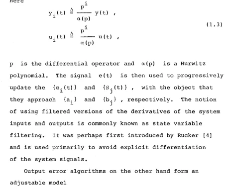
polynomial. The signal e(t) is then used to progressively update the {ot^ (t ) } and { ^ (t ) } , with the object that they approach {a^} and {b ^ } , respectively. The notion of using filtered versions of the derivatives of the system

inputs and outputs is commonly known as state variable filtering. It was perhaps first introduced by Rucker [4] and is used primarily to avoid explicit differentiation of the system signals.

Output error algorithms on the other hand form an adjustable model

~ n_1 ^ m

y (t) + Z a.(t)y. (t) = Z 3 . (t) u.(t) (1.4)

n i=0 1 1 j=0 : 3

with y^(t) obviously defined. The output error

A

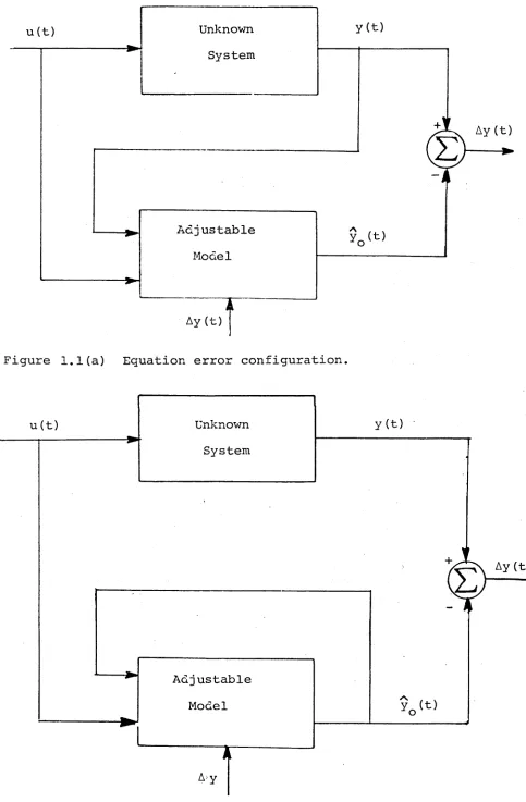
y (t) -y(t) is then used to adjust the parameter estimates {a^(t)} and {(3j(t)} . The difference between equation and output error algorithms is best understood through

Figure 1.1. It is essentially a question of what constitute the inputs to the a d justable model. In equation error the exogenous inputs to this model are three : the unknown system input, the unknown system output and the difference between the outputs of the unknown system and the

system output enters the adjustable model through the

A

output error yQ (t) - y(t), only.

The main disadvantage of equation error algorithms is that they yield biased parameter estimates in the presence of unbiased measurement noise. Output error

algorithms do not have this drawback, but their convergence is conditional on a certain transfer function being

strictly positive real (SPR). Unfortunately, this transfer function depends on the system parameters and hence this condition for convergence cannot always be checked a priori.

Equation error algorithms in their simplest form are typified by those presented by Young [5] and Lion [6]

(Lion calls equation error algorithms using state variable filtering as "generalized equation error" schemes). A

further level of complexity is introduced in the schemes of Narendra and Kudva [7] , Luders and Narendra [8] , Parks [9]

and Caroll and Lindorff [10] . Their schemes lead to the use of fewer integrators and involve the use of positive real transfer functions. Unlike the output error

situation, however, these transfer functions are independent of the unknown parameters and are thus not difficult to

design. Anderson in [11] considers the multivariable extension of these schemes and demonstrates how all of the above [5 - 10] can be unified within the general framework of two prototype structures. As we shall

demonstrate in Chapter 3 these schemes may fail to converge to the right parameter values in the presence of unbounded signals. Schemes suggested by Kreisselmeier [12 - 13]

schemes in [5 - 13] have been derived variously by Morgan and Narendra [14,15] , Kreisselmeier [12, 13] ,

Sondhi and Mitra [16] and Anderson [11,17] . In direct terms their's is a persistently spanning condition on certain regression vectors involving system inputs and outputs. For a system with n+m-1 unknowns, for example, the condition requires that the regression vectors span the entire Rn+m ^ space with time. Intuitively, this translates to a persistence of excitation condition on the system input, even though none of the above results have formalized this assertion.

Persistence of excitation can be viewed as a condition on system identifiability with the proviso that such

identifiability should not be lost asymptotically. This in turn requires that the system be excited by inputs which are sufficiently rich in frequencies. For example, a system with two unknown parameters cannot be identified if the

input is a d.c. signal. On the other hand a sinusoidal input should suffice as it carries with it two pieces of information namely its magnitude and phase.

As we have stated no precise connection between the persistently spanning conditions on the regression vectors and a persistently exciting condition on the system inputs emerges from [14 - 17] . Moreover, the former conditions, with their explicit dependence on the system outputs, are

of this thesis) , has presented persistence Qf excitation conditions on the inputs directly. Similar results, using the technique of Generalized Harmonic analysis have been derived by Boyd et.al. [20,21] . However, whereas the results in this thesis deal also with unstable systems, system stability is crucial to the derivation in [20,21], Discrete time analogues of these results can be found in

[22] .

Discussions of output error algorithms can be found in [23] . Although several discrete time proofs of the

exponential convergence of output error algorithms exist [24, 22] we were unable to find any complete analysis of such convergence in continuous time. In [17,25] error models similar to those arising in output error algorithms are analysed under the implicit assumption of bounded signals. However, since, in principle the

parameters of the adjustable model in (1.4) can vary

arbitrarily, such an assumption seems difficult to justify. In Chapter 5 of this thesis complete analyses of the

output error algorithms is presented.

1.2.2. Adaptive Control

Adaptive controllers can in general be classed into two categories : those employing the indirect and direct

approaches. The former involve the explicit estimation of the system parameters which are then used to design the controller parameters. In the direct approach,on the

other hand,the first phase is sidestepped and the controller parameters are directly estimated.

more difficult than their identification counterparts. This stemmed from the feedback configuration which gave rise to nonlinear, time varying differential equations. The first important contribution in the direct control

area was a model reference scheme for minimum phase plants, proposed by Monopoli [26], who used an augmented error signal to sidestep a positive real condition otherwise implicit in the analysis. These ideas were further

developed by Feuer and Morse [27] , Narendra and Valvani [28], Narendra, Lin and Valvani [29] and Morse [30] . The last two in particular showed global asymptotic convergence of the output tracking error to zero. Their analysis,

however, did not show parameter convergence to the correct values, without which, as we have already asserted,

robustness may not be forthcoming. In [19] it has been shown that with persistently exciting reference inputs, and with known high frequency gain, parameter convergence for [30] not only occurs, but does so exponentially.

Without the knowledge of the high frequency gain, however, exponential stability will not be obtainable. Similar results for the algorithm in [29] have been derived by Boyd et.al. [20,21] .

Äström and co-workers [31 - 33] , Kreisselmeier [34-36], and Elliott and Wolovich[37] in their work have

created indirect algorithms which are globally stable, in that irrespective of the initial parameter estimates the system signals are always bounded. Egardt and Samson [38] in their work considered algorithms having a specific controller but a general identifier satisfying certain assumptions.

the minimum phase requirement is substituted by the

assumption that the extent of a convex region containing the plant parameters, in which the plant is stabilizable and detectable is known.

Recent work by Rohrs et.al.[39] and Äström and

Wittenmark [40] have thrown light upon the behaviour of adaptive controllers in the presence of unmodelled high frequency modes and bounded disturbances. Ioannou [41] and Ioannou and Kokotovic [42] have applied the singular perturbation method to show that the algorithm in [28] retains local stability in face of very high frequency dynamics. Moreover, Narendra and Peterson [43] , Kreisselmeier and Narendra [44] and Sastry [45] have considered the introduction of dead zones in adaptive controllers to tackle bounded disturbances. In [ 4 6 - 4 8 ] error models have been developed, based on which many adaptive controllers have been shown to retain local stability, even in face of departures from some of the idealizing assumptions, as long as the inputs are

persistently exciting.

§1.3 Contributions of this thesis.

As stated earlier the primary objective is to formulate adaptive algorithms for the robust control of systems

multilinear fashion. Thus when two such parameters are unknown, the transfer function becomes

p (s)+k p (s)+k p (s)+k k p (s)

T(s,k ,k ) = -- --- — ---- — — --- (1.5) qQ (s)+k1q 1 (s)+k2q2 ( s) +k][k2q 12 ( s )

where the k^ are the unknown parameters and the polynomials p^(s) and q^(s) are known a priori

This result extends to mechanical and chemical analogues but excludes physical elements such as mutual inductors, which permit cross-coupling between energy storage

devices and elements such as gyrators.

The algorithms we devise thus exploit the intrinsic multilinearity outlined above. As stated above, their

robust behaviour would require that the input signals be persistently exciting (p.e.). However, even in the

simple parametrisation of (1.1) , the p.e. conditions involve system outputs as well. In chapter 3 we develop a set of general tools for translating th^se to input only conditions. The systems for which these tools are applicable include ones which maybe unstable and those which are slowly time varying but have bounded system

signals. These results are appealed to in specialized forms in establishing convergence conditions in the later chapters.

In chapter 4 three equation error algorithms are

through a two parameter example. Assume and are the unknown parameters and consider the vector

A T

K = [k^^k^/k^k^] .o The first steps ignore the dependence of the third element of K on the first two and generate

A T

an "unconstrained" estimate K = [K W K 0,K - . The u ul u2 ul2

second step, which is common to both algorithms then finds

/N A A A A A ip

kp and k^ such that [k^k^fk^k^] is the "closest" to . The third algorithm, on the other hand, combines these two steps into one by using penalty functions ideas. Chapter 5 presents two output error algorithms, based on the first two methods outlined above. These are analysed for uniform asymptotic convergence under the assumption of known parameter magnitude bounds. Chapter 6 presents two

indirect adaptive controllers, both of which employ the same, general controller, but differ in the identifiers used. One is shown to be globally stable while stability of the second is established under assumptions similar to those in [ 3 6 ] , In all algorithms of chapters 4 - 6 , persistence of excitation conditions, which yield global uniform asymptotic parameter convergence, are presented.

§1.4 Notation of this thesis:

In this thesis, for the sake of clarity, notation shall be abused on several counts. To begin with quantities like

v(t) = a(s). u(t)

V(t' b(s)

shall refer to the solutions of the differential equation

b (p) v (t) = a (p) u (t) , A d

p = , with arbitrary but finite initial conditions. In vectors such as

V (t) 4 {• y ft) 7 sy (t) sn 1y(t)> u(t) , . .smu(t) ^ T Cs+a)n (s+a)n (s+a)n (s+a)n (s+a)n

or

W(t) = [ U (t) , s+ß

U(t) .T (s+P)n+m

the initial conditions shall be assumed to be zero. Also v(s) will refer to the Laplace transform of v(t) .

We shall often use sets as subscripts for denoting elements of a vector. For example, the elements of a vector

shall be denoted by K where r is a set. Thus if J ur

r = {1,2} K will K n _ .

ur ul2

Ay (t)

Ay (t) U n k n o w n

S y s t e m

M o d e l

F i g u r e 1.1(a) E q u a t i o n e r r o r c o n f i g u r a t i o n .

Ay (t)

Adj u s t a b l e M o d e l

U n k n o w n S y s t e m

References for Chapter 1

1. B.D.O. Anderson, "Adaptive systems, lack of persistence of excitation and bursting phenomena". Submitted to Automatica. 2. B.D.O. Anderson and R.M. Johnstone, "when Will adaptive

systems really adapt? The robustness issue",Proc. 2nd Conf. Control Engg, IE Australia, 1982, pp 59-66

3. W. Hahn, Stability of motion, Berlin, Springer Verlag, 1967. 4. R.A. Rucker,"Real time system identification in the presence

of noise". Proc. Western Electronics Conv,Paper 2-3,Aug, 1963. 5. P.C. Young,"Discussion on 'In flight dynamic checkout' by

J.E. Walker", IEEE Trans. Aerospace, AS-2, No. 3, pp 1106-1 1106-11106-11106-1.

6. P.M. Lion, "Rapid identification of linear and nonlinear systems", AIAA Journal,vol 5, Oct 1967, pp 1835- 1842. 7. K.S. Narendra and P. Kudva, "Stable adaptive schemes for

system identification and control - parts I and II",IEEE Trans Systems Man Cyber, vol SMC-4, pp 542-560, Nov 1974. 8. G. Luders and K.S. Narendra, "Stable adaptive schemes for

estimation and identification of linear systems", IEEE Trans Auto Contr, AC-19, pp 841-847, Dec 1974.

9. P.C. Parks, "Lyapunov redesign of model reference adaptive control systems", IEEE Trans Aut Contr, AC-11, No. 3,pp

362-367, 1966.

10. R.L. Carroll and D.P. Lindorff, "An adaptive observer for single input single output linear systems", IEEE Trans Auto Contr., AC-18, NO. 5, pp 428-435, 1973.

11. B.D.O. Anderson, "An approach to multivariable system identification", Automatica, vol 13, pp 401-408,1977. 12. G. Kreisselmeier, "Adaptive observers with arbitrary

13. G. Kreisselmeier, "Algebraic separation in realizing a linear state feedback control law by means of adaptive observers", IEEE Trans Auto Cont, AC-25, April 1980, pp 238-243.

14. A .P . Morgan and K.S. Narendra, "On the uniform asymptotic stability of certain linear nonautonomous differential equations", SIAM J Contr, vol 15, Jan 1977, pp 5-24. 15. A .P . Morgan and K.S. Narendra, "on the stability of non­

autonomous differential equations &=(A+B(t))x with skew- symmetric matrix B(t)", SIAM J Cont Opt, vol 15, Jan 1977 pp 163-176.

16. M.M. Sondhi and D. Mitra, "New results on the performance of a well known class of adaptive filters", Proc. IEEE, vol 64, Nov 76, pp 1583-1597.

17. B.D.O. Anderson, "Exponential stability of linear

equations arising in adaptive identification", IEEE Trans Auto Cont, AC-22, Feb 1977, pp 83-88.

18. J.S.C. Yuan and W.M. Wonham, "Probing signals for model reference identification", IEEE Trans Auto Cont, AC-22, Aug 1977, pp 530-538.

19. S. Dasgupta, B.D.O. Anderson and A.C. Tsoi, "Input condi­ tions for continuous time adaptive system problems", Proc 22nd CPC,San Antonio, Texas, Dec 1983. Submitted to IEEE Trans Auto Contr.

20. S. Boyd and S. Sastry, "Necessary and sufficient conditions for parameter convergence in adaptive control", Tech.

Report, University of California, Berkeley, UCB/ERL M84/25, 1984.

22. B.D.O. Anderson and C.R. Johnson Jr., "Exponential

convergence of adaptive identification and control algo­ rithms", Automaatica, vol 18, Jan 1982, pp 1-13.

23. Y.D. Landau, Adaptive control: the model reference approach Marcel Dekker, Inc., 1979.

24. C.R. Johnson, Jr.," A convergence proof for a hyperstable adaptive recursive filter", IEEE Trans Info Thy, vol IT-25 Nov 1979, pp 746-749.

25. K.S. Narendra and L.S, Valvani, "A comparison of Lyapunov and hyperstability approaches to adaptive control of

continuous systems", April, 1980, pp 243-247, AC-25.

26. R.V. Monopoli, "Model reference adaptive control with an augmented error signal", IEEE Trans Auto Cont, AC-19,pp 474-484, October 1974.

27. A. Feuer and A.S. Morse, "Adaptive control of single input single output linear systems", IEEE Trans Auto Contr, AC-23 pp 557-570, Aug 1978.

28. K.S. Narendra and L.S. Valvani, "Stable adaptive controller design- direct control", IEEE Trans Auto Contr, AC-23,pp 570 - 583, Aug 1978.

29. K.S. Narendra, Y.H. Lin and L.S. Valavani, "Stable adaptive controller design - part II :Proof of stability",AC-25, pp 440-448, June 1980.

30. A.S. Morse, "Global stability of parameter adaptive control systems", IEEE Trans Aut Contr, AC-25, pp 433-440, June 1980. 31. K.J. Astrom and B. Wittenmark, "On self-tuning regulator",

Automatica,N o . 8, pp 185-199, 1973.

"Theory and applications of self tuning regulators Automatica, vol 13, pp 457-476, 1977.

33. K.J. Astrom, B .Westerberg, B. Wittenmark,"Self - tuning controllers based on pole placement design", CODEN:

LUTFD2/(tfrt-3148)/1-52/ Department of Automatic Control Lund Inst, of Tech, Sweden, 1978.

34. G. Kreisselmeier, "Adaptive control via adaptive observation and asymptotic feedback matrix synthesis," IEEE Trans

Auto Contr,AC-25, pp 712-722, Aug 1980.

35. G. Kreisselmeier, "On Adaptive state regulation", IEEE Trans Auto Contr, AC-27, pp 3-16, Feb, 1982.

36. G. Kreisselmeier, "An approach to stable indirect adaptive control", Submitted for publication.

37. H. Elliot and W.A. Wolovich, "Parameter adaptive

identification and control", IEEE Trans Auto Contr, AC-24, pp 592-599, Aug 1979.

38. B. Egardt and C. Samson,"Stable adaptive control of non-mimimum phase systems", Systems And Control Letters, vol 2 pp 137-144, Oct. 1982.

39. C. Rohrs, L.S. Valavani and M. Athans, "Convergence studies of adaptive control algorithms, part I: Analysis," Proc CPC, Albuquerque, New Mexico, 1980, pp 1138-1141.

40. K.J. Astrom, "Analysis of Rohrs counterexamples to adaptive control", Proc. 22nd CPC, San Antonio, Texas, vol 2,pp 982-987, Dec 1983.

41. P. Ioannou, Robustness of model reference adaptive schemes with respect to modelling errors, Ph.D. Thesis, University of Illinois at Urbana-Champaign, August 1982.

Singular perturbations and robustness of control systems, Lake Ohrid, Yugoslavia, July 1982.

43. B.B. Peterson and K.S. Narendra, "Bounded error adaptive control", IEEE Trans Auto Contr, AC-27 1982 pp 1161-1168. 44. G. Kreisselmeier and K.S. Narendra, "Stable model reference

adaptive control in the presence of bounded disturbances", IEEE Trans Auto Contr ,ac-27, 1982, pp 1169-1176.

45. S. Sastry,"Model reference adaptive control- stability, parameter convergence and robustness", Tech. Report,

University of California at Berkeley, No. UCB/ERL M83/59, 1983.

46. R.L. Kosut, C.R.Johnson, Jr. and B.D.O. Anderson, "Robust­ ness of reduced-order adaptive model following", Workshop on applications of adaptive systems theory, Yale

University, 1983.

47. R.L. Kosut, C.R. Johnson,Jr. and B.D.O. Anderson,

"Conditions for local stability and robustness of adaptive control systems", Proc. 22nd CPC, San Antonio 1983, pp 972-976.

48. C.R. Johnson, Jr., B.D.O. Anderson and R.R. Bitmead, "A model reference adaptive controller formulated for local optimality in non-ideal use", Presented at the 18th Conf.

§2. Realization Theory

The purpose of this chapter is to motivate the form of models to which the adaptive algorithms of this thesis are applicable. As stated earlier the object is to

arrive at parameterizations which involve quantities with direct physical relevance. Accordingly, this chapter analyses the way in which physical element values of lumped linear electric circuits appear in state variable realizations and transfer function descriptions. Extensions to mechanical and chemical analogues are then immediate.

The primary goal is to show that when most parts of a linear, time-invariant, finite-dimensional system are known,but certain parameters associated with physical components of the system are unknown, then the transfer function of the system can be viewed as a ratio of two polynomials, with the polynomial coefficients multilinear

in the unknown parameters. For example, with three unknown parameters, the transfer function of a single input

single output (SISO) system is of the form P(s,k ,k ,k )

T(s-k ,k ,k ) = --- --- ---— ; (2.1) 1 1 J Q(s,k1,k2,k3)

P(s1,k1,k2,k3) = pQ (s)+k1p1(s)+k2p2(s)+k3p3(s)+k1k2p1 2(s)

+ k1k3p1 3(s) + k2k3p2 3(s)+k1k2k3p1 2 3(s) and

Q(s,k1,k2,k3)=qo (s)+k1q1 (s )+k2q2 *s ^+k3q 3 (s )+k1k2qi2

Here, are the unknown parameters, the polynomials p^(s) and q^(s) are known a priori and T is

proper.

As a means of establishing this property we shall first examine the manner in which the state variable realizations of the systems in question are affected by these unknown parameters. In particular it will be shown that such parameters appear in state variable realizations in a rank-1 fashion, the definition of which is given below.

Definition 2.1

A state variable realization described by the quadruple {F,G ,H ,J } has a rank-1 dependence on N parameters

k^,...,k if for all i G {1,...,N} g a^,b^ G ^ '

independent of k^ , such that if we define by either

1

a . = ---1 a . + k . b .

l l i

or

k..

l

a . =

---1 a . + k .b .

l l i

then the following hold :

(i) The elements of F,G,H and J are multilinear in the a . .

l

(ii) The matrices

si - F G

-H j

Remark:

(2.1) The and defined above may depend on k . V i # j .

3 J

In section 2.1 we shall establish this rank-1 property for electrical circuits. This will be done by examining in turn electric circuits having :

(i) resistor, inductor and capacitor (RLC) elements only, and no capacitor loops or inductor cutsets.

(ii) the above elements and possibly also pathologies such as inductor cutsets and capacitor loops.

In section 2.2 the corresponding transfer function result for the SISO case will be given while, in section 2.3

we shall also show that most electric circuits will retain this transfer function property even if one is unable to make definite statements about the state variable

realizations. This result will pre-suppose the existence of certain input-output descriptions.

The contents of this chapter are the subject of [1] .

2.1 State variable realizations:

Much of the background material for this section,

namely the construction of state variable realizations for electric circuits, is contained in [2,ppl56-209]. We shall show that by following the general construction procedure outlined in [2] we arrive at state variable realizations which obey the rank-1 property.

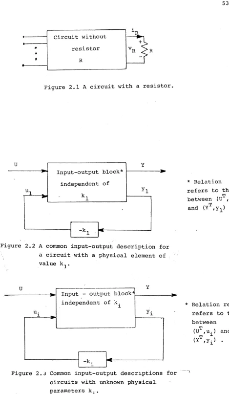
rest of the circuit in a manner depicted in figure 2.1. Now,suppose U is a vector of inputs having a set of voltages or currents at the n-ports as its elements. Similarly suppose Y is an output vector, containing a disjoint set of voltages and currents as its elements. Suppose also that u- and y., are v_ and i0 ,

respectively (v and i are the respective voltage across

K K

and current through the resistor R) . Then, if the hybrid

T T T T

matrix relating [U ,u^] to [Y ,y^] exists, the input-output description typified by figure 2.2 exists. In

figure 2.2, k ^ = R . Sometimes, when the hybrid

T T T T

description relating [U ,u^] to [Y ,y ] does not exist, one may need to replace by , with u^ = iR

and Yi = v r * Similarly other element values can also be extracted, in most circuits, in a manner typified by

figure 2.1, though u^ and y^ may not necessarily represent voltages and currents. The exceptions to this rule arise from element values like mutual inductors, which allow crosscoupling to occur between different energy

storage elements or from elements such as gyrators . In this section, however, we are only interested in extracting resistor values, in a manner depicted in

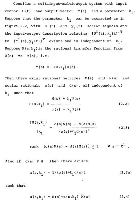
figure 2.2. The following lemma indicates the special way in which the parameter kp extractable as in figure 2.2, affects input-output description relating U and Y . Here, as in the rest of the thesis we shall abuse notation by denoting U(s) , for example, to be the Laplace transform of U (t) . Similarly H(s)U(t) will denote the inverse

Lemma 2.1

Consider a multiinput-multioutput system with input

vector U(t) and output vector Y(t) and a parameter .

Suppose that the parameter k^ can be extracted as in

figure 2.2, with u^ (t) and y^(t) scalar signals and

T T

the input-output description relating [U (t),u (t)]

T T

to [Y (t),y^(t)] exists and is independent of k^ .

Suppose H(s,k^)is the rational transfer function from

U(s) to Y(s) , i.e.

Y(s) = H(s,k1 )U(s) .

Then there exist rational matrices M(s) and N(s) and

scalar rationals c(s) and d(s), all independent of

k^ such that

M (s ) + k^N(s)

H ( s , k 1 ) = --- (2.2)

c (s) + k ^ d (s)

3H(s,k1 ) c (s )N (s) - d(s)M(s)

--- = --- (2.3)

3k1 { c (s)+k d (s) } 2

rank (c(s)N(s) - d(s)M(s)} < 1 V s C .

Also if d(s) £ 0 then there exists

a(s,k^) = 1 / {c(s)+k^d(s ) }

such that

(2.3a)

rank M(-) < 1 . Similarly if c(s) £ 0 then there exists

ot(s,k1 ) = k 1 /(c (s)+k1d(s) )

such that

A / \

H ( s , k 1 ) = H(s) + a( s , k 1)M(s) (2.5)

H(s), M (s ) independent of a(s,k^) and rank M(») < 1 .

Pr o o f .

Suppose

'Y(s) 'h 11 ( s ) h 1 2 (s)- ~ U(s)

y x (s > _{h 2 1 (s) h 2 2 <S)} Y 1 (s)

where H ^ ( s ) is a matrix, h ^ 2 (s) and h 2^(s)

vectors and h 2 2 (s) a scalar. Thus

y 1 (s) = h 2 1 (s) U (s ) - k 1h 2 2 (s) y ^ s )

whence

Y(s)

k h ( s ) h (s)

[H1 n ( s ) + ^ --- ]

1 + k lh 2 2 (s*

U(s) (2.7)

from which (2.2) and (2.3) follow with c(s) = 1

3H(s,k1 ) h 22 (s)h12 (s)h21 (s)

3'sk^ 1 + k 1h 22 (s)

with a defined as in (2.3a) . Thus (2.4) follows.

Similarly (2.5) also follows. VVV

Remarks

(2.2) Replacing k n by ^/, does not alter the

1 K 1

conclusions of the lemma, though (2.4) and (2.5)

will be interchanged.

(2.3) If k^ is a resistor value then a(s,k^) is

independent of s .

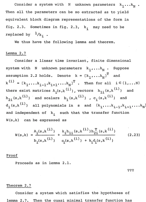
Consider now a circuit having N parameter values,

k-...k.T such that each k. can be extracted so that

I N l

input-output description of the form in figure 2.3 exist,

with U and Y containing appropriate currents and

voltages as their elements. Then the following lemma

extends the result of lemma 2.1 to this case.

Lemma 2.2

Consider a system with input vector U(t) and output

vector Y (t ) and N parameters k^,...,k . Suppose

each parameter can be extracted so that input-output

descriptions of the form of figure 2.3 exist. Define

k = [k^, .. . ,k ] T and k (i> = [k1 , T

* **^i-l'^i+i'* *

Then V i 3 c. (s,k^^) and d . (s , k

l ^ ) , rational scalars

in s and elements of

•H

such that every element of

H(s,k) , defined by

is multilinear in the {a.} with a. defined as

l l

l/(c .(s,k ^ ) + k^d^ (s,k ^ ) ) or

or k . / (c . ( s , k ^ ) + k . d . ( s , k ^ ) ) .

l i l i

Remark:

(2.4) The correspond to the in lemma 2.1, the first definition of ou will not apply if d^ = 0 and the second if c. = 0 . If neither c. nor d. is

l l i

zero then the lemma holds for defined either way.

Proof

Consider an arbitrary element h^(s,k) of H(s,k) . Then from (2.4) or (2.5) of lemma 2.1, we have that

h (s,k) = h ^ ^ ^ ( s , k ^ ^ ) + a . m ^ ( s , k ^ ) (2.8)

pq pq i pq

where h ^ and m ^ ^ are independent of a. . Consider

pq pq i

h (s,k) = h 8, (s ,k ( } ) + a. m Ä <s,k<£)) (2.9)

pq pq £ pq

— z £

where h and m are independent of a„ but not

pq pq ^ £

— ( £ )

in . Thus a simple argument shows that h and (Z)

m are also affine in a. and that h is

pq l pq

bilinear in and for all i and Z, i ^ Z . Proceeding along these lines the result follows.

vvv

2.1.1. RLC circuits with no pathologies:

Consider an n-port RLC circuit having n^ inputs and nQ outputs. Suppose that all input and output quantities are either port currents or port voltages. Denote u to be the n^ dimensional input vector and y to be the nQ dimensional output vector and assume that the elements of u and y do not overlap. Augment u and y to form the n-dimensional input and output vectors U and Y respectively, in the following manner. Assign all elements of u and y to U and Y respectively.

th

Suppose that the j port current is an input. Then t h

assign the j port voltage to Y . Similarly, if the th

j port current is an output then assign the corresponding voltage to U . If for a particular port neither the

current nor the voltage are in either of u or y , then assign one of these arbitrarily to U and the other to Y. In this way for every port either the voltage or the

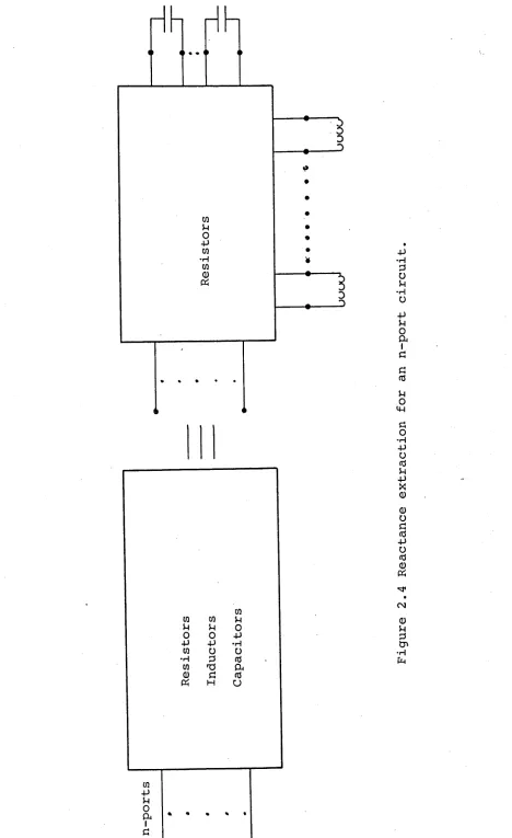
current appears in U and the other appears in Y . Consider next the following reactance extraction procedure illustrated in figure 2.4. Suppose there are

n inductors and n capacitors in the circuit in question,

i-i c

Form the vectors U , U , Y and Y in the following

C C -Li

t h

way. Assign the voltage across the j capacitor to th

th

corresponding voltage to the j element of . Now, suppose all the capacitor and inductor connections were open-circuited. Then we are left with an n + n + n

Li C

circuit containing resistors only. Then denoting

[UT ,UT ,U?]T and [YT ,YT ,Y?']T as input and output vectors

c li c Li

respectively, define M

as the hybrid matrix relating the two, i.e.

Y M

11 M12 M13 U

Y

c = M21 M22 M2 3 Uc (2.

y l M31 M32 M33 UL

Since, the network relating the two vectors is resistive, M is non-dynamic. Moreover, it has been shown in [2]

that with Y, Y , Y , U, U and U selected as above

C Li C -Li

M exists and is unique, whenever the RLC circuit we started with is free of inductor cutsets and capacitor loops. Indeed the existence and uniqueness of this M is the standing assumption for this sub-section.

Assumption 2.1

with Y ' V y l' u ’ V y l

M exists and is unique.

Theorem 2.1

Consider an RLC circuit having n inductors and

Xj .

nc capacitors, with quantities y, Y, Yc , YL , u, U, U , UL and M defined as above. Suppose, assumption 2.1 holds.

Then the (n^+n^)-dimensional state variable representation T T T

having u and y as input and output and [U ,U ] as

c J_i

the state vector, has a rank-1 dependence on all the inductor, capacitor and resistor values appearing in the circuit.

Proof:

We first show that the state variable representation

• T T T

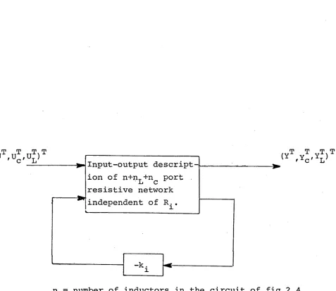
Suppose is a resistance appearing in the

reactance extracted network. Then as argued before an input-output description of the form in figure 2.5 is possible. Then by lemma 2.1 there exist a^,b_^ R such that with = R^/(a^+R^b_^) or ou =

V(

1 c

Al be diagonal matrices having all the capacitor and

inductor values respectively. Then provided that elements

a l u l

as the input, output

and state vectors respectively, the following representation results :

: a l are appropr

Y = A Ü and

c c c

U , Y and T T 1

fU c ’U L ]

x = Fx + GU Y = Hx + JU where

(2.11)

H = [M

12 M 13J1 11

Clearly, if we choose a to be i

capacitor value and a = J_j .

V

1 C . L .

in (2 Hence the result follows.

for each

each inductor value in a rank-1 fashion.

2.1.2 RLC circuits with inductor cutsets and capacitor loops

Suppose inductor cutsets and capacitor loops do appear in the circuits in question. Then from [2] it is clear that assumption 1 need not hold. As it turns out

reactance extraction is still possible but Uc ,UL ,Yc and Y need to be redefined.

i-i

Suppose the reactance extracted n+nc+nL port circuit has (n+nL+nc)-dimenstional input and output vectors U and Y respectively. Suppose also that all the elements of U , defined in the previous section, are in U and all

_ th

the elements of Y are in Y . Also if the j capacitor or inductor current appears in U then the corresponding voltage appears in Y and vice versa. Then by [2]

there always exists a selection of U and Y such that with M defined as

Y = M Ü

M exists and is unique. Clearly M is also non-dynamic. Moreover, U and Y can be partitioned as

_m m m m m m

ir = [tr,u* , u* ,tr , uT ]

c i L 1 c 2 L 2

and

— T Y 1

where U and U carry, respectively, those of the

C 1 L 1

capacitor voltages and inductor currents which have been assigned to U . As before, if any element of U or

U is a voltage then the corresponding element of Y

I_j • c

1

or Y is a current and vice versa. Then the Li •

1

following theorem is true.

Theorem 2.2

Consider an RLC circuit with input u and output y and with U,Y,U ,Y ,U ,Y ,U ,Y ,U ,Y and M

1 1 L 1 h l 2 2 L 2 L2

defined as above. Suppose n and n are the dimensions

C 1 L 1

of U and U respectively and that M exists and

C 1 1

is unique. Suppose also that the transfer function relating U to Y is proper. Then the (n +nT )

C 1 1 dimensional state variable realization of

T T T

the circuit, having, u,y and [U ,U ] as the input, C 1 L 1

output and state vectors respectively, has a rank-1 dependence on the elements of the circuit.

Proof:

As in theorem 2.1 we first show that the state T T T variable realization having U, Y and [U ,U ] as

C 1 1

the input, output and state vectors respectively, has a rank-1 dependence on the circuit elements. From this the result will follow. According to [2]

where

i4

— T — — T

- M, . and M . = - MI! .

4i i5 5i Now as in

the proof of theorem 2.1 we see that for every resistor there exists cu such that 9M/3ou has rank-1 with respect to a . .

l

Now if the column IVL^. is dependent on ou then the elements row M _ . cannot be as the

5i

are zero. Moreover M.,_ =

M.„ M C[_, M . _ and M_ .

44, 55 45 54

— T

- M 5i Thus the fourth and fifth rows and columns are independent of all

Moreover, from [2] we have that the following state space realization is possible, where x T T

[Uc '°£ ] 1 L 1

x = D - ^ x + D - 1 (D3-D2D - 1D 4D 5 )U

y = (D6+ DjD 4D ” 1D 2 )x+ [ D 7-D6d" 1D 3 + (2.13)

D 5D 4D 11(D3_ D 2D 11d4D 5 )]U + ° 5 (D8~D 4D 1^ 4 > °5Ö

Here

D 1

with Al obviously defined;

D

6 13

D 7

T -1

and Dg - positive definite symmetric. Thus if the T T -1

system is proper D,_ (Dg-D^D^ D4)D5 and hence D5 must be zero. Thus (2.13) can be rewritten (see [2]) as

X = D _1D 2x + D ^ D g U

(2.14) y = D x + D_U

D /

Clearly, as is independent of a

i

the state-variable realization in (2.14) has a rank-1

dependence on all ou . Consider any capacitor or inductor in set 1, i.e. in the set whose elements are represented in

Let this be . Then

T

= D + k^e^e.. for some j

where e . 3 and B 11

4" Vi

Thus

T -1 , , k . D. te .e .Dt _ D-x = D-1 . „X 11 3 3 ^

1+k.e.D.,e. i 3 1 1 3

- k

so that with a

1+k . e . D, t e . 1 3 11 J the rank-1 property is satisfied

Similarly for an element k. in set 2

D1 = °12 + kiXxT

where x and are independent of k^ and x is a

v e c t o r .

Thus

-1 -1

— - 1 -- T - 1

k i ° 1 2 X X °12

_ _t _

1 + k.x D -„ X

l 12

whence with a _{_ _}

t —

1+k.x D, ~x

l 12

the rank-1 property holds.

v v v

The above results were derived purely from the standpoint

of electric circuits. However, as we have already stated the

Given are the dynamics pertinent to the attitude control of the communications technology satellite, Hermes

[

].

x = Ax + BU

Y = Cx

where

A 0 1 0 0

a)0h / I 1 0 0 w0 -h/I2

0 0 0 1

0 h / I 2-u)0 -w0h/12 0

B

F iL lG lCosa^ I l 0

F lL lG lsina/I2 F2L2G2/ I2

C = 0

0

0 0

Here $ is the roll, \p the yaw, I the moment of inertia about the roll axis, I2 , that about the yaw axis, o)0 the orbital rate, h the nominal wheel angular momentum, a the offset angle, and

F2 the offset and yaw thruster levels respectively,

L 1 and L2 the offset and yaw thruster moment arms respectively and G1 and G2 the impulse bit factors. The inputs u-^ and u2 provide a guide for the level of consumed fuel.

It is evident that the parameters Ii,J2 ,F^,^2 ,L^,L2 ,G1 and G2 appear in the state variable representation in a rank-1 fashion. Although

sI-A I B

I T

---C j o

has rank-1, the system matrix is obviously not multilinear in a . Thus a does not quite conform to the definition of rank-1 dependence. The parameters o)o and h , on the other hand, clearly do not appear in a rank-1 fashion. But, by definition (one is the orbital rate and the other the wheel angular momentum) one can see that they must allow cross-coupling between energy storage elements. They thus fall in the same category as mutual inductors or gyrators, which as we have emphasized do not appear in state variable realizations in a rank-1 fashion.

2.2 Transfer functions for SISO systems

In this section we show that rank-1 SISO systems have minimal transfer function descriptions typified by (2.1). To begin our analysis we consider first the manner in which

_3_

a single parameter appearing in a rank-1 system affects the transfer function.

At the outset we introduce the following definition of coprimeness of polynomials in more than one variable:

Definition 2.2

Consider p (X^, . . . Xr,Xn+^ / • • • xm ) and q(X^,...Xn ,

X ^ f...Xm ) which are polynomials in the indeterminates Xl'***Xm * T^en P an<3 <3 are coprime with respect to the variables X . ....X if there exist no nontrivial f, which

--- 1-i---- n i

is a polynomial in x i'*’*xn • rational in Xn+l'**'Xm such that

f l f 2 = P

and

flf 3 = *

with f2 and f^ , polynomials in x i'***xn anc^ nationals in X ...X . a s well. The extension to the case where

n+1 m

the coprimeness of more than two polynomials is in question is obvious.

The following theorem shows that a system having a state variable realization which has a rank-1 dependence on a

single parameter a has a transfer function whose numerator and denominator are affine in a .

Theorem 2.3

x = F ( a ^ ) x + g(a^)u

T

y = h (a^) x + j (a^) u

w i t h a system m a t r i x of the form

s I - F U - ^ j g tc^)

I

f s I - F Jg O 1 ^ o

1

1—

1

Ö

+

' V

r rp 1 1

9i 1 g 2

~1

- h T (a1 ) | j (ax )

1---T 1 .

- h Jj

O 1 o _ _ h 2 _

(2.15)

where F0 • 90 '^o' -^o '^1 '^2 ' ^1 anc^ ^2 independent of a, has

a transfer function

a (s) + a,b (s)

W (s) = --- ----- (2.16)

c (s ) + a 1d(s)

for every . The polynomials a(s),b(s),c(s) and d(s) are

independent of and obey the following restrictions:

(a) 6[c(s)] = n, 6[d(s)] < n, 6[a(s)] < n and 6[b(s)]< n

(b) a(s)d(s) - b(s)c(s) is factorizable into two polynomials

of degree not exceeding n .

Conversely, any transfer function of the form (2.16) has a state variable realization of the form (2.15) provided that conditions (a) and (b) hold.

P r o o f :

(i) From equation (2.15)

2

W(s) = [a(s)c(s) + a^{a(s)d(s) + g2h 2c (s) - h2y(s)c(s)

where

a (s) c (s)

h T (sI - F ) 1 g + j

o o Jo

c(s) = det (si - F )

d (s) c (s)

Y (s) c (s)

3 (s) c (s)

g l (sI _ F o r l h l

T -1

g n (si - F ) g

T -1

h (si - F ) ± h,

o o' 1

^ (2.18)

We note that

a (s) d (s) + g 2h2c (s ) “ h 2y(s)c(s) + g 2 $(s)c(s) - y(s)3(s)

=

)

)

- (

is divisible by c(s) because

W (s) a(s)/c(s) 3 (s) /c (s) ”h T l o

Y(s)/c(s) d(s)/c (s) T

L g iJ

-1

[ s I-Fo ] [g h ]

_ th

Thus W(s) has an n ord e r r e a l ization and its M a c m i l l a n degree is not greater than n . Thus ad-3y is d i v i s i b l e by c(s) whence (2.19) is div i s i b l e by c(s) . Define b (s) by

Then (2.17) has the same form as (2.16) and by (2.20) and

(2.18) condi t i o n s (a) and (b) are satisfied.

(ii) Suppose that (a) and (b) h o l d for (2.16). Let

a (s) d (s) - b (s) c (s) = f 1 (s)f2 (s) = (y(s) - g 2c(s)) (3(s)

+ h 2c (s))

w ith 6 [ 3 (s)] and 6[y(s) ] < n . Then a(s)d(s) - f^ ( s ) f 2 (s) is

divisible by c(s) wh e n c e

W(s)

a(s)/c(s) f2 (s)/c(s)

f 1 (s)/c(s) d(s)/c(s)

has M a c m i l l a n degree not greater than n .

A

Hence W(s) can be e x p r e s s e d as

r , T i r -1

h sI-F g h.. I + j h 0

o L o J _ o 1 J J o 2

T

g i - _"g 2 0

so that by reversing the a r gument in the first part of this

t h e o r e m a state variable r e a l i z a t i o n of (2.16) exists in

the form t y p i f i e d by (2.15). VVV

Remark

(2.5) The reverse i m p l i c a t i o n of theorem 2.3 is

interesting. It shows that not all transfer functions w h o s e

n u m e rator and d e n o m i n a t o r p o l y nomials are affine in ot^ ,

have state variable descrip t i o n s w h i c h have rank-1

dependence on

1 *

-b (s) s 3 + 1

and a(s) and d(s) are such that

a(s)d(s) = 6s4 - 2s3 + ils(i)2 + 5 . Then

a(s)d(s) - b (s)c (s) = (s2+l) (s2 + 2) (s2+3) .

Thus there do not exist f-^s) and f2 (s) of degree less than or equal to 3 , for which

a (s) d (s) - b (s) c (s) = f1 (s)f2 (s)

is true. Thus

a (s) + a,b (s) W(s) = ----

----c(s) + a1d(s)

has no state variable realization which has a rank-1

dependence on a . In general one of the following three conditions obtain:

(i) If 6[b(s)] < 6[c(s)3 = n then <5[a(s)d(s) -b(s)c(s)] < 2n - 1 (as 6[d(s)]<n) . Thus a(s)d(s) - b(s)c(s) is always expressible as a product of two polynomials of degree less than or equal to n .

(ii) If 6[b(sj] = n and n is even, then again f^(s) and f2 (s) will have degree no greater than n .