LiDAL: Light Detection and Localization
AUBIDA A. AL-HAMEED 1, SAFWAN HAFEEDH YOUNUS 1, AHMED TAHA HUSSEIN1,
MOHAMMED THAMER ALRESHEED2, AND JAAFAR M. H. ELMIRGHANI 1
1School of Electronic and Electrical Engineering, University of Leeds, Leeds LS2 9JT, U.K. 2Department of Electrical Engineering, King Saud University, Riyadh 11451, Saudi Arabia
Corresponding author: Jaafar M. H. Elmirghani ([email protected])
This work was supported in part by the Engineering and Physical Sciences Research Council (ESPRC), INTERNET (EP/H040536/1), STAR (EP/K016873/1) and TOWS (EP/S016570/1) projects.
ABSTRACT In this paper, we present the first indoor light-based detection and localization system that builds on concepts from radio detection and ranging (radar) making use of the expected growth in the use and adoption of visible light communication (VLC), which can provide the infrastructure for our Light Detection and Localization (LiDAL) system. Our system enables active detection, counting, and localization of people, in addition to being fully compatible with the existing VLC systems. In order to detect human (targets), LiDAL uses the visible light spectrum. It sends pulses using a VLC transmitter and analyses the reflected signal collected by a photodetector receiver. Although we examine the use of the visible spectrum here, LiDAL can be used in the infrared spectrum and other parts of the light spectrum. We introduce LiDAL with different transmitter-receiver configurations and optimum and sub-optimum detectors considering the fluctuation of the received reflected signal from the target in the presence of Gaussian noise. We design an efficient multiple input multiple output (MIMO) LiDAL system with a wide field of view (FOV) single photodetector receiver, and also design a multiple input single output (MISO) LiDAL system with an imaging receiver to eliminate the ambiguity in target detection and localization. We develop models for the human body and its reflections and consider the impact of the color and texture of the cloth used as well as the impact of target mobility. A number of detection and localization methods are developed for our LiDAL system, including cross correlation and a background subtraction method. These methods are considered to distinguish a mobile target from the ambient reflections due to background obstacles (furniture) in a realistic indoor environment.
INDEX TERMS Optical indoor localization, VLC systems, people detection, counting, localization, optimum receviers.
I. INTRODUCTION
Visible Light Communication (VLC) systems are used to provide illumination and data communications. VLC uses light emitting diodes (LEDs) or lasers to encode data into light intensity in the visible spectrum [1]–[5]. VLC systems have many advantages such as cost-effectiveness using the existing lighting infrastructure, operating on a broad, unli-censed bandwidth, security (light signals do not penetrate walls) and there is no interference with Radio Frequency (RF) signals [4], [6]–[8].
People counting has become an emerging and attractive area in the past decade [9], [10]. Many approaches have been developed for counting in public places such as subways, bus stations and supermarkets [10], [11]. The outcome of
The associate editor coordinating the review of this manuscript and approving it for publication was Chunbo Xiu.
these techniques can be used for public security, resources allocation and marketing decisions. Passive infrared (PIR) imaging systems have been employed to detect and count people, however, the PIR system is temperature dependent, thus leading to a vast number of detection failures [11], [12]. Other passive optical detection methods were studied that rely on detecting the shadow of subjects to determine the position of the subject [13]. These approaches show good accuracy in the presence of a single object, however the presence of multiple moving shadows can be an issue, and there is a need to carefully position the illumination sources for good positioning. Ultra-wideband (UWB) radar has been utilized to effectively detect and track outdoor pedestrians. However, for an indoor environment, the effects of signal scattering and absorption by obstacles significantly impairs the performance of UWB indoor radar [11], [14]. IR Laser detection and rang-ing (LADAR) has been used to detect people by monitorrang-ing
the reflected signal patterns of people legs [11]. Counting systems based on computer vision and digital image process-ing are becomprocess-ing meanprocess-ingful and useful. Video cameras with image processing algorithms have been widely used to count people indoor and count pedestrians outdoor [10], [14], [15]. It should be noted however that acquiring images of people poses in many cases privacy concerns, whereas our LiDAL system uses light reflections from people and therefore no images of people are acquired, stored or transmitted.
In this paper, we introduce for the first time indoor light-based detection, counting and localization of people light-based on the use of radar-like reflections. This can significantly expand the utility of indoor VLC systems. The key concept behind our LiDAL system is the use of the (visible) light reflected from targets (people) where the light reflectivity is a function of the material type and colour of the target’s surface. The reflected light signal is captured by a photodetector which monitors the change in the light intensity in the time domain. LiDAL can be a system embedded in the VLC system to provide additional functionality to detect, count and local-ize people. In addition, LiDAL reduces the complexity and cost associated with the acquisition and digital processing of images to detect the presence of people.
To the authors’ best knowledge, the proposed system is the first to employ an indoor optical radar for people detection and localization. It uses the visible light spectrum associated with VLC systems, and can potentially use other parts of the light spectrum. It is worth noting that the use of the infrared spectrum for example can eliminate issues with light dimming and switching off light sources. The concept of LiDAL has the benefits of active radio waves used in radar systems while avoiding, as mentioned, the issues associated with UWB (and other radio) radar signal propagation indoor. It also makes use of the existing lighting / illumination sys-tems and potentially the existing VLC syssys-tems infrastructure. Due to the fact that (visible) light is reflected from opaque objects, the major critical issue in LiDAL is how to distin-guish the people (targets) from other background objects, i.e., furniture. In order to overcome this problem, we have considered the mobility of people as a key distinguishing feature between humans and furniture. Even in the case of nomadic users, people exhibit movement of body parts while stationary, for example while sat working in an office environment. They may also standup from time to time. We introduced a background subtraction method and a cross-correlation method for target detection when targets are mobile. The contributions of this work can be summarized as follows:
1) We proposed for the first time an indoor (visible) light pulsed radar-like system which utilises the VLC sys-tem transmitters to detect, count and localize multiple targets.
2) We developed a model for the human body and its reflections and the impact of the colour and texture of the clothing used, which are all important attributes of the target of interest.
3) We considered a range of different mobility models for humans and used these as an important input to our LiDAL human detection and localization system. 4) We designed optimum and sub-optimum receivers and
algorithms for the proposed LiDAL systems.
5) We designed MIMO-LiDAL and MISO-Imaging-LiDAL systems which are compatible with VLC and light fidelity (Li-Fi) systems.
We would like to note that the current work is analytic and simulation in nature. It is however the first work to the best of our knowledge that uses radar-like techniques to detect and localize people indoor. We intend to conduct experimental demonstrations in the future.
We would also like to note that we have adopted a staged approach in the introduction of the concepts; (i) as this is the first treatment, we believe, of radar-like concepts for localization indoor using light and (ii) we believe that this approach can help the reader understand the boundaries. For example, we initially consider and then build on a system that is not able to achieve localization such as the single input single output system. This system illustrates the principles, but does not have enough measurements/equations to achieve localization. We also allocate space to cases such as the case of a single target in an empty room and multiple targets in an empty room, which are later seen to be special cases of multiple targets with obstacles.
This paper is divided into sections as follows: Section II introduces the modeling of the environment and the targets. Section III presents the analysis of LiDAL system range, resolution and optimum and sub-optimum receiver design. Section IV presents target distinguishing approaches and mobility modeling in a realistic environment. Section V develops the design of MIMO-LiDAL systems. Section VI considers the design of the MISO-IMG-LiDAL system. Section VII presents the simulation setup and results. Finally, conclusions are drawn in Section VIII.
II. REALISTIC ENVIRONMENT AND TARGET MODELLING To study the performance of the proposed LiDAL system, simulations were performed in a typical office consisting of a furnished room, with dimensions of 4 m (width) ×
FIGURE 1. (a) Realistic simulation environment setup and (b) basic 3D target model.
illumination standards. Each unit had 9 RGB laser diodes (LDs), and the total transmitted power from each RGB-LDs light unit was 18 W [20], [21], [22]. It is worth mentioning that, each light unit consists of red, green and blue laser diodes which are driven by different modulation currents to meet the illumination standards [20], [21]. It is also worth noting that the light engine has a diffuser infront of the RGB laser diodes and the radiation pattern emitted is thus lambertian. This lambertian pattern was measured and verified experimentally in [23]. The work in [23] consid-ered RGB laser diodes and employed them for illumination. We have also discussed the design of this light engine in [20]. It is also worth noting that a single colour can be used for our localisation (radar) application, however all three (RGB) colors are needed for illumination.
[image:3.576.39.275.63.374.2]The average target (person) dimensions considered were 15 cm ×48 cm ×170 cm (depth×width ×height) [24] as shown in Fig.1b and colored polyester fabric was con-sidered as the target coating material. The fabric reflection model used was based on the work in [25], which ana-lyzed the reflections from different types of fabric includ-ing silk, cotton, polyester, acetate and glass fiber. We also made use of the work in [26] which examined the combina-tion of fabric colour and material and their impact on light reflection. The resulting reflections in [25] were observed to be a combination of diffuse (Lambertian) and specular
TABLE 1.Reflection model for a different target coating materials [17].
reflections. In [25], the distribution of the reflected visible light of several cloth materials was experimentally studied. In particular, cotton reflectance was about 9% specular and 91% diffuse, while polyester reflectance was 10% specular, 26% diffuse and 63% internal multiple reflections which are treated as diffuse reflections as can be seen in Table 1. It should be noted that 1% of the polyester reflections are internal reflections which occur inside the fabric layers [25]. Therefore, in our simulation, we only considered a Lamber-tian pattern (i.e. diffuse) as the model for the target’s surface material. The reflectivity factor of different dyed polyester fabrics ranges between 0.25 and 0.72 [26]. Moreover, the reflectivity of dark and white human skin is 0.04-0.35 and 0.16-0.86 respectively [27]. Regarding furniture, office desks (1.54 m (width)×0.76 m (length) × 0.75 m (height)) and a bookshelf (3 m×0.8 m×2 m) are considered, and are located in the room as shown in Fig.1a, where the office desks and bookshelf materials were finished-wood with a reflectivity factor of 0.55 and diffuse reflections [28]. The Lambertain diffuse reflections order for the furniture and target is assumed to be 1.
III. LiDAL SYSTEM
In this section, we analyze the LiDAL system maximum range which is related to the receiver’s field of view. We also pay attention to the received reflected signal in two LiDAL configurations that relate to the colocation or separation of transmitter and receiver in space. Furthermore, we analyze the resolution and the ambiguity of target detection which are related to the transmitted pulse width. In addition, we exam-ine the optical receiver design for LiDAL and consider the receiver bandwidth and thermal and ambient noises. In our LiDAL system, the sources of randomness are attributed to the target colour of cloth, the target orientation and the receiver noise. Note that in terms of indoor optical wireless channel, we consider the channel at the target’s maximum range dictated by the receiver field of view (and the receiver sensitivity). The fluctuation of the received reflected signal attributed to the different colors worn by the target is modeled leading to a pdf of the target reflection factor. The target (human) random orientation and its impact on reflections was determined through extensive simulations, leading to a pdf of the effective target cross-section. The optimum LiDAL receiver is then formulated using Bayes structures and signal space theory for single and multiple targets in the presence of the impairments outlined above.
A. RANGE ANALYSIS
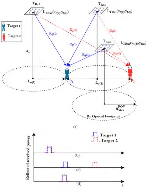
FIGURE 2. LiDAL range and reflection analysis: (a) a spaced transmitter-receiver (bistatic) arrangement placed on room ceiling with a target located near the transmitter at a distance ofRFOVMaxfrom the receiver; (b) a spaced transmitter-receiver placed on room ceiling with a target located away from the transmitter at a distance ofRFOVMaxfrom the receiver; (c) and (d) collocated transmitter-receiver (monostatic) arrangement placed on room ceiling with a target at two locations.
floor. An optical receiver, collocated or separated from the transmitter, collects the received reflected pulses. The received signal is a superposition of the reflected pulses from the target(s), static environment obstacles (furniture) and noise. Note that, in this section we assumed the target(s) are located in an ideal environment (i.e. an empty room with zero reflectively from walls, ceiling and floor). Therefore, the received reflected signal randomness is only due to tar-get(s) colors and effective cross-section and is corrupted by noise. In Section III we deal with the presence of furniture (reflections) and reflections from the walls.
The maximum range of LiDAL can be determined depend-ing on the receiver’s photodetector FOV. The maximum range
RFOVMax for a certain receiver concentrator FOV (9c) is given as
(see Fig. 2):
RFOVMax =tan(9c)(do−h) (1)
where9cis the semi-angle of photodetector’s concentrator,
do is the perpendicular distance between the ith receiver
location LRxi (xRxi ,yiRx,ziRx) and the ground reference point
Loi(xoi,yio,0) as shown in Fig. 2 andhis the target height. Fig. 2 presents two different possible transmitter and receiver configurations with a target located inside the receiver optical footprint (i.e. receiver FOV). We refer to the collocated transmitter-receiver configuration as ‘monostatic LiDAL’ and refer to the spaced transmitter-receiver configu-ration as ‘bistatic LIDAL’.
The received reflected optical power (PBr RFOV
Max
) from a target
at maximum range, i.e., located in the receiver optical foot-print at a radius ofRFOVMax, for a bistatic LIDAL (see Fig. 2a, b) is derived as:
PBr RFOV
Max
=(n+1)(nele+1)
4π2R2 1R22
Gc(9c)PtdAρAR
×cosn(θ)cos(ϕ)cosnele(ϕ
and for monostatic LiDAL (see Fig. 2c, d), PMr RFOVMax
is
written as:
PMr RFOVMax
= (n+1)(nele+1)
4π2(d
o−h)2+RFOV
2
Max 2
×Gc(9c)PtdAρARcosn+3(9c) (3)
whereR1is the distance between the transmitter and target,
R2 is the distance between the target and receiver, R2 =
(do−h)2+RFOV
2
Max 12
,Gc(9c)is the gain of the
concentra-tor,Ptis the transmitted power,dAis target cross section area
(top and/or the sides),ARis the photodetector physical area,
ρis the target reflection coefficient,θandϕare the angles of irradiance and incidence respectively,neleis the Lambertain
order for the target diffuse reflector andnis the Lambertian emission factor of VLC light source defined as [29]:
n= − ln(2)
ln(cos(8)). (4)
The gain of the concentratorGc(9c)is given as [30]:
Gc(9)=
N2
sin2(9c)
(5)
where8 is the semi-angle at half power of the VLC light source (8 > 9c) andN is the concentrator refractive index.
It should be noted that the transmitter has a broad radiation pattern (n = 0.52 for illumination purposes [20], [21]) and the target assumed has a diffuse emission factor ofnele=1.
Therefore, the target has a narrow radiation pattern com-pared to the transmitter’s radiation pattern. With such narrow radiation pattern, the target delivers maximum power to the receiver if it is directly under or near the receiver. As such, the weakest received reflected signal from a target occurs when the target is at the edge of the receiver FOV (i.e. target located atRFOVMax).
The photodetector area (AR) and the concentrator’s FOV
and gain are among the receiver’s key parameters that deter-mine the LiDAL detection performance. The values of these parameters have to satisfy the LiDAL (radar) design require-ments. We analyze their impacts later in this paper. In addi-tion, the transmitted powerPt is set at the maximum power
needed for normal illumination in the room. (i.e.Pt =18W
according to the design in [20]). We therefore do not consider in this paper the impact of dimming on our LiDAL system, and in cases where dimming is an issue, infrared sources and detectors can be used for LiDAL.
B. RECEIVER BANDWIDTH
To determine the maximum receiver bandwidth needed, we selected the LiDAL configurations that result in the largest channel bandwidths which the receiver has to deal with. The largest channel bandwidths occur when the target is under the receiver. We have also evaluated, through simulation, the channel bandwidths at a large number of target locations. Figs. 3a and b show a target located underneath the receiver
for the LiDAL bistatic and monostatic scenarios respectively. We have simulated the pulse dispersion associated with the bistatic and monostatic LiDAL channels due to target pres-ence at different target locations. The target’s locations have been generated uniformly inside the receiver optical foot-print (see Figs.3a and b) to calculate the channel impulse response and then to obtain the 3dB channel bandwidth for each location. It should be noted that we considered an ideal indoor environment without furniture or background obstacles, and we treated the room’s floor as a non-reflective surface (i.e. zero reflection factor). In addition, the simulation and calculations of the received reflected signal were carried out using MATLAB. Our simulation tool is similar to the one developed by Barry [30] in terms of the indoor channel impulse response calculation method. Figs. 3c and 3d depict the probability distribution of the channel bandwidth (Bwch)
for the bistatic and monostatic LiDAL systems respectively. As can be seen in Figs. 3c and 3d, the bistatic LiDAL chan-nel is more dispersive than the monostatic LiDAL chanchan-nel due to the large distance between the transmitter, target and receiver. Table 2 summarizes the bistatic and monostatic LiDAL channels characteristics.
TABLE 2.Characteristics of LiDAL channel.
We calculated the channel bandwidth for the monostatic and bistatic LiDAL systems as follows:
1) An input pulsepl(τ) with time duration τ of 0.01ns (equal to the time bin duration used in the simulation [31]) is presented to the input of a transmitter unit, RGB-LDs, with impulse responsehtx(t)followed by
calculation ofHtx(f)=F(htx(t))F(pl(τ)). It is worth
mentioning that, the RGB-LDs have a large bandwidth (few GHz) [20] and therefore, given a channel with few hundred MHz bandwidth, we ignored the laser transfer function.
2) We set the following simulation parameters for the monostatic and bistatic LiDAL systems: The room has dimensions of 8m ×4m ×3m and the illumination requirements were met using 8 light units distributed as shown in Fig. 1a. These light units also represent the LiDAL receiver locations. To provide overlapping LiDAL coverage zones, the receiver FOV was set to 43◦. The transmitter beamwidth was set 75◦ for illumination purposes [21] and the impulse response was calculated with a time bin of 0.01ns duration. The monostatic transmitter-receiver pair was located at (2m, 4m, 3m) at the center of the room in Fig.1a. The bistatic transmitter was located at (2m, 5m, 3m) and the receiver was located at (2m, 4m, 3m).
3) We calculated the LiDAL channel impulse response
FIGURE 3. LiDAL channel configurations (a) Tx and Rx placed in different locations (bistatic) with a target located at the center of the optical footprint, (b) Tx and Rx placed in the same location (monostatic) and a target located at the center of the optical footprint, (c) the histogram of the received power in bistatic LiDAL versus bandwidth and (d) histogram of the received power in monostatic LiDAL versus bandwidth.
target present) using the ray tracing propagation model in [29], [30], [32], [33]. In this paper, we considered the first and second order reflection components in the sim-ulation of the impulse response of the LiDAL channel. We then determined the 3dB channel bandwidth,Bwch,
usinghch(t) .
4) The required 3dB receiver bandwidth is determined as
BwRx=max Htx(f)|3dB,Hch(f)|3dB
(6)
C. LiDAL RESOLUTION AND AMBIGUITY IN TARGET DETECTION ANALYSIS
The distance (R1) between the monostatic LiDAL transceiver
unit (TRx) and the target is calculated based on the round trip
time (i.e. time taken by the pulse from the transmitter to the target plus the time taken by the reflected pulse back from the target to the receiver),ttrip, and the speed of light,c, as:
R1=
cttrip
2 . (7)
The range resolution of LiDAL is defined as the minimum separation distance (1R) at which two or more targets can be reliably detected as illustrated in Fig. 4. The range reso-lution is related to the pulse width of the transmitted signal.
FIGURE 4. The LiDAL resolution needed to distinguish two targets.
The LiDAL resolution (1R) is given as [34]:
1R=R1,1−R1,2=
cτ
FIGURE 5. The reflected received signal current from two targets located in an empty room in a monostatic LiDAL configuration.
whereτ is the transmitted pulse width. The separation dis-tance1xybetween two targets, as can be seen in Fig. 4, is given as:
1xy=R1,1sinθ1,1−R1,2sinθ1,2 (9)
and ifθ1,1∼=θ1,2=θ,then
1xy= R1,1−R1,2sinθ=1Rsinθ. (10)
Therefore,1xy ≤ 1R, and in a typical room such as that in Fig. 1a, we determined thatθ = 430, hence here1xy ≤
0.681R.
Fig. 5 shows an example, a simulation, of the received pulse response attributed to the reflected signal, as received by a transceiver (TRx) unit which covers an optical footprint
that includes two targets in the presence of noise. In this work, we considered typical room layouts, where for example in a meeting room (closest separation between people in a business setting), the designers recommend an inter-chair-distance more than 60cm as in [35] and 75cm as in [36], and the typical justifiable distance between two people having a conversation is 30 cm. Therefore, we selected a minimum LiDAL resolution of1R = 30cm and therefore given (10),
1xy ≤ 30cm which is the required minimum separation between two targets (i.e. the requiredτ is 2ns from (8)). Opti-cal transmitters and optiOpti-cal receivers that support this band-width are readily available, and the optical wireless channel is able to provide such bandwidth [37], [38]. The analysis of the channel bandwidth for the bistatic and monostatic LiDAL systems (see Fig. 3c, 3d) showed high channel dispersion and low channel bandwidth which cannot accommodate a transmitted pulse of 2ns duration without pulse spreading in the receiver. Thus, an equalizer is required to mitigate the imperfections of the LiDAL channel.
Let us first assume an ideal indoor environment (i.e. no reflected signal from the room’s background). Here
ambiguity in multiple targets detection occurs when the dis-tance between targets is less than the LiDAL (radar) resolu-tion1R. In other words, when the difference of the targets’ round trip times is less than the transmitted pulse width
ttrip(1)−ttrip(2) < τ
.
This leads to ambiguity. Further-more, the ambiguity in target detection is affected by the configurations of the LiDAL system.
Table 3 provides a comparison between conventional radar and LiDAL when the only available information is range. Note that the angle of arrival in LiDAL can be determined through coherent optical detection, but this is too complex, and is not considered here. As Table 3 shows, complete local-ization is only achieved when three or more anchor points are available to provide range estimations.
D. RECEIVER NOISE
We considered the receiver bandwidth needed in Section B, here we consider receiver noise in LiDAL.
In optical wireless (OW) systems, the noise can be divided into two components, a shot noise (σshot2 ) component and a thermal noise component (σthermal2 ). The total noise variance
σ2
t is given by [17], [29]:
σ2
t =σthermal2 +σshot2 . (11)
The shot noise variance is defined as the sum of contributions from the ambient lights (direct sunlight, desk lamps etc.) and the noise from the received signal. The shot noise, σshot2 , is written as [39]:
σ2
shot =2qBwRx Ib+RespPr (12)
whereqis the electronic charge,BwRx is the receiver
band-width,Respis the photodiode responsivity andIbis the
back-ground current due to ambient lights. We considered the effects of shot noise due to desk-lamps. For the four office desk-lamps shown in Fig. 1a, we considered Philips light bulbs where each light bulb has an optical power of 13w [40]. The background current measured in [40] wasIb =
TABLE 3. LiDAL localization compared to traditional radar localization.
the visible spectrum can be used to reduce the background noise to comparable levels. In addition, an electrical high pass filter can be implemented to reduce the DC component of the ambient noise. However, these solutions may increase the cost and the complexity of the LiDAL receiver. We have not used an optical bandpass filter and have not used an electrical high pass filter to simplify the system design.
In this work, the optical receiver was a siliconp-i-n pho-todetector with a transimpedance amplifier (TIA), selected to achieve high sensitivity and a good dynamic range [41], [42]. The receiver considered in this work had high speed and low input noise, designed by Texas InstrumentsR [43].The TIA with aBwRxof 300 MHz had a thermal input noise current of
about 2.5 pA/√Hz [43].
E. RECEIVED SIGNAL FLUCTUATION AND TARGET REFLECTIVITY MODELLING
The fluctuation of the received optical power reflected from a target is related to the target coating reflection factor (ρ) (i.e. colour, material type and, reflection type) and the target effective cross section area (Ae). The target effective cross
section area is the size of the target surface area illumined by the transmitted pulse (which reflects light) and depends on the target position, LiDAL transmitter and receiver con-figurations and LiDAL field of view. It should be noted that,
the fluctuation of the received signal due to target reflection factor (colour of clothing and type of clothing worn) is inde-pendent of the target position and the target orientation (i.e., independent of the target effective cross section area).
Table 4 presents a range of people favorite colors with the weights associated with each colour and reflection factors for dyed cotton coating material [44], [45]. The people favorite colors weights show features of a Gaussian distribution, Fig. 6. This can be explained by observing that the received reflected signals over an extended period of operation of the LiDAL system will be due to multiple colors and coating materials worn by the person (target) in every case; and this together with the large number of subjects allow the central limit theorem to be involved. Therefore, we fitted and optimized the survey data of the people favorite colors using a Gaussian distribution as can be seen in Fig. 6 where, the target reflection factor is the random variable of the distribution. The survey data of favorite colors [44], [45] was fitted to minimize the root mean square error (RMSE), and the minimum RMSE obtained was about 15%.
The probability distribution function (PDF) of the target reflection factorp(ρ)is given as:
p(ρ)= 1 σρ
√
2πe −
(ρ−µρ)2
2σ2
ρ
TABLE 4. People favouratie colors survey data.
FIGURE 6. The PDF of target reflection factor.
where,µρ andσρare the mean and standard deviation of the target reflection factor respectively.
We determined the PDF of the effective target cross section area through simulation. The target shown in Fig. 1b (human body model) was placed at a large number of locations in the room and the ray tracing indoor propagation method of [17], [46], [47] was used to determine the power reflected by all the target surface area elements for the given target location and orientation, and the given LiDAL transmitter and receiver configurations. We then fitted the simulated data to a nor-malized Gaussian distribution as can be seen in Fig. 7 where the target is placed randomly in the receiver optical footprint edge at different locations and with different orientations. At each location, the target is rotated to eight directions with a step size of 45◦angle randomly. The minimum RMSE of the effective target cross section area fitting obtained was 5%. The PDF of the effective target cross section areap(Ae)is
written as:
p(Ae)=
1
σAd √
2πe
− (Ae−µAe) 2
2σAe2 !
(14)
where,µAe andσAe are the mean and standard deviation of
the target effective cross section area respectively. Observing
FIGURE 7. The PDF of the effective target cross section area.
the results in Fig. 7, it can be seen that the effective target cross section area variation is small with aσAe = 4 and a
large meanµAe=50. Thus, the average value of target cross
section area is used. In other words, the target effective cross section area is modeled as a random viable with mean (µAe)
and very small variance, which is ignored.
The received reflected signal from target is given as:
Pr=Aoρ (15)
where, Ao is the LiDAL channel gain for a target located
atRFOVMax as in equations (2) and (3) of bistatic and monas-tic LiDAL systems respectively; and ρ is a Gaussian ran-dom variable described in equation (13). Thus, the PDF of the received reflected signalp(Pr) without noise can be
defined as:
p(Pr)=
1
σs √
2πe −
(Pr−µ)2
2σs
(16)
where, (µ=Aoσρ) and (σs =Aoσρ) are the mean and
stan-dard deviation of the received reflected signal. Equation (16) represents a Gaussian random variable scaled by a positive constant representing the LiDAL channel gain for a target located atRFOVMax.
In the OW channel, ambient light induces shot noise in the photodetector receiver in addition to the thermal noise of the receiver amplifier. This noise is modeled as a white Gaussian noise [29] with zero mean and variance ofσt2(see equation 6). The noise probability density is given as:
p(n)= √1
2πσt
e
−
n2
2σ2
t
(17)
wherenis the total detected noise current in the receiver and
σtis the noise current standard deviation.
density of the received signal in the presence of noisep prn
is written as:
p prn
= 1
q
σ2 s +σt2
√
2π
e
−
(Pr−µ)2
2(σ2
s+σt2)
(18)
where,µand
q
σ2 s +σt2
are the mean and standard devia-tion of the received reflected random signal in noise.
F. LiDAL OPTIMUM RECEIVER DESIGN
We used Bayes receivers and signal space theory to design an optimum receiver structure for LiDAL taking into account the minimization of the average cost of making decisions and the error in target detection. We then design a sub-optimum receiver. Bayes criterion takes into account the impact of the cost of making a wrong decision in different LiDAL applications by setting an optimum detection threshold. For the sub-optimum receiver we also establish detection thresholds.
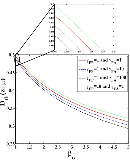
For instance, in a people counting application the cost of miss-detecting people may be low, however, for a LiDAL security application the cost of miss-detecting a target may be very high. We employed signal space techniques with a max-imum posterior probability (MAP) decision rule to design an optimum LiDAL receiver based on minimum probability of error to detect target(s) for multiple cases as we discuss later in this paper. In addition, We evaluated the performance of the optimum detection threshold Dth(z) where the random
variablezrepresents the received power in (18).
1) OPTIMUM DETECTION THRESHOLD ANALYSIS (HARD DECISION)
We analyzed the optimum detection threshold for the LiDAL receiver considering the fluctuation of the received reflected signal and the cost of making a decision on LiDAL given the application considered. In LiDAL, the goal is to decide the presence or absence of a received reflected signal from a target in the presence of noise. This situation can be cast into two hypotheses. LetH1represent the hypothesis where
noise is present and the reflected signal (from the target) is absent. Let H2 represent the hypothesis where both the
received signal (from target) and noise are present. The PDF ofH1can be written as:
Fz(z|H1)=
1
√
2πσt
e
−
z2
2σt2
(19)
and the PDF ofH2is given as:
Fz(z|H2)=
1
√
2πσe −
(z−µ)2
2σ2
(20)
where,σ2andµare the variance and the mean of the received signal inH2withσ2= σs2+σt2
, see equation (18).
The Bayesian average cost of making decisionC(D)is given as [48], [49]:
C(D)=(poα21+qoα22)+ Z
(qo(α12−α22)Fz(z|H2)
−(po(α21−α11)Fz(z|H1)))dz (21)
where, po and qo are the prior probabilities of H1 andH2
respectively. For LiDAL, we define the four prior costs as:α11 which is the cost of deciding that the target is absent when it is true,α22 is the cost of deciding the target
is present when it is true,α12is the cost of deciding the target
is absent when it is false andα21 is the cost of deciding the
target is present when it is false. It should be observed that
poandqowere set to 0.5 which is a general case where it is
equally likely to have a target or no target (for example in an indoor environment). In particular dense (user wise) indoor environmentsqomay be higher thanpoand the converse is
true in sparse indoor environments. Therefore, the parameters can be determined accordingly. We are interested in the costs of wrong decisions (α12andα21), hence we assumedα11and
α22 (costs of correct decisions) are equal to zero. To clarify
this,α12is defined as the cost of missing a target, whileα21is
defined as the cost of a false alarm. Note that,α12 should be
set higher thanα21,for security applications where missing a
target is worse than a false alarm. However we are interested here in target counting applications, and thereforeα12was set
equal toα21 where both wrong decisions equally contribute
to wrong counting. Thus, the LiDAL average cost of making decisionC(D)VLPcan be written as:
C(D)VLP
=poα21+
qoα12 Z
Fz(z|H2)dz−poα21 Z
Fz(z|H1)dz
.
(22)
The first term of (22) represents the fixed cost while the sec-ond term represents the variable cost. We wish to minimize the second term of (22) by choosing the value ofz. Mathe-matically (22) can be summarized by a pair of inequalities, and can thus be rewritten as:
qoα12Fz(z|H2) H1
≶ H2
poα21Fz(z|H1) . (23)
For LiDAL, we defineγFA and γFP as the cost factors of
missing the target and false alarm respectively. Therefore,γFA
(FA is False Absence) is given as:
γFA=qOα12 (24)
and theγFP(FP is False Presence) is given as:
γFP=pOα21. (25)
Thus, we get:
Fz(z|H2)
Fz(z|H1) H1 ≶ H2 γFP γFA (26)
whereγFP
γFA is the LiDAL likelihood test threshold, and Fz(z|H2)
FIGURE 8. The Optimum detection threshold withβσand LiDAL cost factors.
Substituting equations (19) and (20) into equation (26), the optimum detection thresholdDth can be derived as (27), as
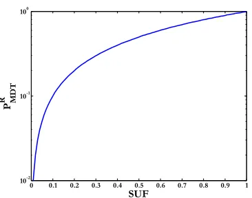
shown at the bottom of this page, where, we define βσ = σ2
s+σt2
σ2
t
as a colour factor whereβσ ≥1. The colour factor
βσ is a measure of the variation in the received reflected sig-nal due to the colour worn by the target, versus the variation in the received signal due to noise. For example, if all the targets wore the same colour, thenσs2=0 andβσ =1. At the other extreme, if the colors worn by the targets are very different and the receiver noise is very small,βσ → ∞. It is worth observing that in addition to colour, other optical properties of the target coating affect βσ, such as the material used in the clothing (e.g. cotton verses polyester).
As can be noted in Fig. 8, when the weights of cost factors are equal (γFP
γFA = 1) andβσ ≈ 1 (i.e. the value of signal
variance is very small σs ≈ 0), the optimum Dth ≈ µ2.
This case is the classical scenario [49], which acts to vali-date our derivation of equation (27). Fig. 8 shows the main operating region for the LiDAL detection system. Firstly, the LiDAL system can be used for counting purposes only. In other words, to count the number of human pedestrians. Here the cost of missing a target and the cost of a false alarm are identical as they result in equal counting errors. This is
represented byγFP=γFA. Secondly, if the application is such
as that there is high cost associated with falsely identifying the presence of a target in the indoor environment, then the detection threshold is set high, represented for example by
γFP = 10 and γFA = 1 in Fig. 8. Finally, if the cost of
missing a human pedestrian target is very high (security or safety application), then the threshold should be set very low as shown in Fig. 8 where for exampleγFP=1 andγFA=10
andγFA=100.
2) LiDAL OPTIMUM DETECTOR
We use the term detector here to imply and include the initial signal detection by the optical receiver, followed by its optimum processing and finally decision making. We imple-mented a MAP detection approach in LiDAL to design an optimum receiver based on observation of the received reflected signal(s); and hence calculation of the posterior probability to minimize the probability of decision errors [48]. In LiDAL, a single transmitted pulse is sent and is reflected from the target(s) to the receiver where the receiver uses a finite listening time. The LiDAL receiver listening time (Ts) is divided into N time slots. Two cases arise,
the single target case and the multiple targets case. In the single target case, (i) if the target presence in all spatial locations is equally likely, then the time slots have equal prior probabilities for target reception; (ii) in the single target case, however, the reception of a pulse in a time slot implies that the remaining time slots (if any) will contain no pulses, hence the independence of the time slots does not hold. In the multiple targets case, condition (i) holds, and further in (ii) the reception of a pulse does not exclude the remaining time slots from having targets / pulses. Therefore, indepen-dence of the time slots can be assumed (ignoring instances where targets may walk in pairs for example). Therefore, we assume here equal prior probabilities for the time slots and assume the independence of the time slots, which is a general common case. The LiDAL receiver has to optimally determine (i) target presence, (ii) number of targets (number of time slots containing pulses) and (iii) identify the time slot (target’s range).
The time slot width (Ts) is related to the desired LiDAL
resolution and target ranging accuracy. Therefore, we select a time slot width equal to the transmitted pulse width (Ts=τ)
in order to obtain a 1R = 30cm resolution. This 30cm resolution corresponds to the minimum typical separation of interest between humans in an indoor environment. Select-ing narrower pulses can improve the resolution, however this is not needed and can lead to higher dispersion in the channel.
Dth H1
≶ H2
v u u u t
µ2
(βσ −1)2
+ µ
2
βσ −1 + 2 σ2
s +σt2
βσ −1
ln
γFP
γFA
−lnq σt
σ2 s +σt2
−
µ
βσ −1
Here we analyze three cases of interest: Single target case, multiple targets case and multiple targets with channel dispersion.
Case I Assumptions:Single target, noise present, no chan-nel dispersion, the receiver’s N time slots are orthogonal (i.e. only one received reflected pulse), the received reflected pulse may fit into a single time slot, or overlap with a neighbor time slot (i.e. the received pulse is shifted in the listening frame depending on target location and may occur at the boundary of the time slot), and independent time slots. For the purpose of this case, the objectives of the designed receiver are detecting the target presence and its range.
Case I is similar to M-ary orthogonal signals (pulse posi-tion modulaposi-tion (PPM)) [49], where a single transmitted pulse is reflected from one target and received by a time slot
Tsj. The MAP rule for minimum probability of error is given
as [48], [49]:
P(Hi|z1, . . .zN)=
fZ(z1, . . .zN|Hi)P(Hi)
fZ(z1, . . .zN)
(28)
where,Z =[z1, ..zN] is the observed received signal vector
inN time slots andP(Hi) is the probability of receivingHi,
withP(Hi) =
1 N+1
,i ∈ {1...,N+1} ;P(Hi)takes this
values since the received reflected signal from a target can be present (equi-probably) in any ofN time slots depending on the target location. Note that,P(Hi) andfZ(z1, . . .zN) do
not depend onHi [48]. Therefore, we require a receiver to
calculatefZ(z1, . . .zN|Hi) and choose theHiassociated with
the largest probability [49]. The orthonormal expansion of the received signal can be written as [49]:
Zj= Z T
0
(pr(t)+n(t)) φj(t)dt j∈ {1, . . .N} (29)
where,pr(t)is the received signal,n(t)is the noise andφj(t)
is the orthonormal basis function chosen as:
Z T
0
φu(t) φj(t)= (
1, u=j
0, u6=j (30)
where,φj(t)=Q(t−jTs). It should be noted thatz1, . . .zN
are uncorrledetd and statistically independent. Therefore their joint probability is given as:
fZ(z1, . . .zN|Hi)= N Y
j=1
Fz zj|Hi
i∈ {1...,N+1} (31)
The mean and variance of hypothesisHiare given as:
EZj|Hi =Aij (32)
varZj|Hi =σ2 (33)
whereAij is the orthonormal coefficient given as [49]:
Aij = Z T
0
pr(t) φj(t)dt (34)
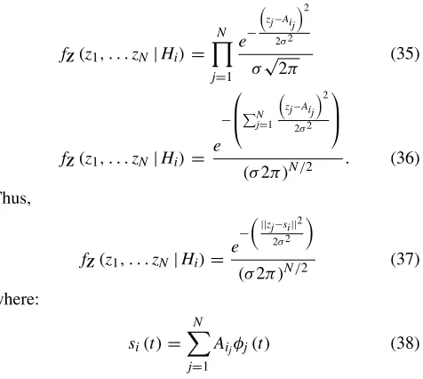
Equation (35) can be rewritten as:
fZ(z1, . . .zN|Hi)= N Y
j=1
e−
zj−Ai j
2
2σ2
σ√2π (35)
fZ(z1, . . .zN|Hi)=
e
−
PN j=1
zj−Ai j
2
2σ2
(σ2π)N/2 . (36) Thus,
fZ(z1, . . .zN|Hi)=
e
− ||
zj−si||2
2σ2
(σ2π)N/2 (37) where:
si(t)= N X
j=1
Aijφj(t) (38)
Therefore, as equation (37) shows, the optimum receiver that maximizes the likelihood is one that minimizes the dis-tance betweenzandsi. In other words, it is a receiver that
chooses the minimum distance to the orthonormal coefficient coordinates.
For instance whenN =2, we have three hypotheses: (i)H0
no target and both time slots contain only noise (note equation 19 forFz(z|H1)), (ii)H1time slotTs1 contains the received reflected signal form a target with noise and Ts2 contains only noise and (iii)H2time slotTs1 contains only noise and
Ts2 contains the received reflected signal with noise. The receiver decision rule for H1 and H2 will be to compare
the values of zj to the orthonormal coefficient values and
select the minimum distance to the orthonormal coefficients as illustrated in Table V. However, for H0 all time slots
[image:12.576.302.540.79.292.2](i.e.zjvalues) have comparable energy.
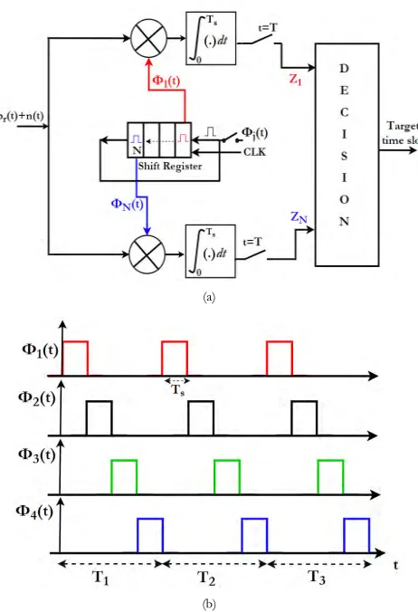
Fig. 9a shows the optimum LiDAL receiver structure to be used to detect a single target (see Case I) based on the analysis of Table 5 and equation (29). Each branch uses one of the orthonormal functions (see shift register) and an integrator to determine theN dimensional expansion point collectively between the branches. Therefore, after observing the received signal inN time slots during the listening time (T = NTs),
the receiver decides the target presence and range (related to
Tsj) through the decision circuit. Fig. 9b presents an example
of the orthonormal functionsφj(t)forN =4 time slots with
Ts=2ns for three radar (LiDAL) scans during theTlistening
time.
FIGURE 9. LiDAL receiver, (a) The LiDAL optimum detector block diagram, single target detection and (b) the orthonormalφj tsignaling diagram.
We evaluated the performance of the LiDAL receiver through the probability of making a correct decisionPc on
Hi, where the reflected signal from the target is received as
zi;Pccan be derived as:
Pc=P zi|Hj
=P(zj>zm) where∀m∈ {1, ..N},m6=j.
(39)
Substituting equations (29) and (17) in equation (39), we get:
Pc=
Z Dth
−∞
e
− n
2
j
2σ2
t
!
√
2πσt
dnj
N−1
. (40)
Case II Assumptions:Multiple targets, target locations are spaced by 1R or more, noise is present, no channel dis-persion, the receiver N time slots are orthogonal, but the received multiple reflected pulses fromk targets (k ≤ N) may be shifted depending on the targets locations and hence the received pulses are not orthogonal. We do not consider the case where there are more targets than time slots, which is an extension that warrants further investigation. We consider this situation however in the imaging receiver case in Section V.
a: EXHAUSTIVE SEARCH RECEIVER (ESR)
In this section, we propose an optimum receiver for Case II based on an exhaustive search algorithm as follows:
1. The receiver observes the reflected signalpr and
pro-duces the orthonormal expansionZfor theNtime slots in the presence of noise.
2. First, the receiver’s decision block (as can be seen in Fig. 9a) compares these N orthonormal coeffi-cients coordinates to the ‘no target’ hypothesis as all
N time slots contain only noise, where the observed
N orthonormal coordinates are (z1,z2..zN) and the
orthonormal coefficient are (Av1,Av2, ..AvN). For the
no target case, Aij = 0,∀j and the error ev can be
defined as:
ev= XN
j=1||zj−Avj||
2 (41)
3. The decision block then compares the observed N
orthonormal coefficients coordinates to the coefficients associated with the presence of a single target hypothe-sis; where there areNpossible time slots to receive the reflected signal from the target, yieldingN candidate answers; and calculate their errors (see equation (41)). 4. Next, the decision block calculates the errors assuming the presence of two targets, where there areN(N2−1) candidate answers. Thus, the total candidate answers (CA) forN time slots andktargets can be defined as:
CA=1+ N X
k=1
N!
(N−k)!k! N ≥k (42)
5. Finally the decision block continues to find the errors for all cases and chooses thevthcase (number of targets and their time slots) which has the minimum error:
v=arg min
v CA X
v=1
ev !
v∈ {1, ..CA} (43)
For example, a LiDAL system with listening time divided into N = 14 time slots and maximum counted targets of
k=10, the total candidate answers areCA =15914.
There-fore, the exhaustive search receiver may be very complex to implement for the LIDAL system. It should be noted however that the exhaustive search receiver visits and compares all the possible answers and thus its probability of correct decisions converges to that in (40), [49].
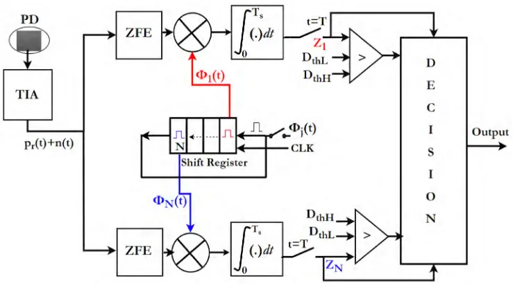
b: SUB-OPTIMUM RECEIVER (SOR)
[image:13.576.41.272.66.404.2]In this section, we introduce a sub-optimum receiver with lower complexity compared to the exhaustive search receiver. Following the analysis of the MAP rules, Fig. 10 presents the sub-optimum receiver for Case II. For the sake of simplifying the analysis of Case II, let us assume two targets,k = 2, detection inN = 2 time slots. Hence, we have four hypotheses: (i)H0noise present only and targets
are absent,(ii) H1a single target is present atTs1 with noise,
FIGURE 10. The LiDAL sub-optimum receiver block diagram.
TABLE 6. Multiple targets detection hypotheses with N time slots.
(iv) H3 two targets present at Ts1 and Ts2 with noise. Table 6 illustrates the four possible hypotheses and receiver observation with the decision. To determine H0 with
min-imum error, a comparator is connected at the output of each correlator to determine the presence/absence of the received reflected signal at each time slot compared to a lower detection threshold DthL as can be seen in Fig. 10.
In addition, the receiver has to determine whether there is a single reflected pulse located between two neigh-boring time slots (i.e. the correct decision is H1 or H2)
or there are two reflected pulses from two targets received in the two time slots (i.e. the correct decision isH3).
Conse-quently, we set up a second comparator at the output of each correlator with a high detection thresholdDthH =
µ
2 as can be
seen in Fig. 10. Therefore, the final receiver decision block decides as follows:
1. If the observed received signal zj is belowDthL, then
the target is absent inTsj.
2. If the observed received signalzj is aboveDthH, then
the target is present inTsj.
3. If the observed received signal zj is above DthL and
belowDthH, then it is a pulse received in two
neigh-boring time slots Tsj,Tsj+1. Thus the decision circuit compareszjwithzj+1and selects the largest.
It should be noted that the lower threshold,DthL, is selected
based on the application and the acceptable probabilities of false alarms and misses. This is discussed in detail in
Section V where the results in Fig. 20 and Fig. 21 are used to select the detection threshold. For example, if false alarms are to be avoided, a high threshold should be set. This however leads to missing targets. In our current application, the pur-pose is to count people and therefore high false alarms are accepted to ensure that every target is counted and localized. For example, we chose in Section V a high false alarm probability of 0.1. This led (from Fig. 20) to a detection probability of 0.92 and hence a threshold of 0.32 times the received signal, where the evaluation was done at maxi-mum range. In terms of the high detection threshold,DthH,
the worst detection case occurs when a pulse is received in a position such that it is exactly equally split between two neighboring slots. We have thus set the high detection threshold to half the received power in this sub-optimum receiver.
TABLE 7. ZFE delay spread and noise enhancement.
To eliminate the effect of the inter-time slots interfer-ence (ITI), the receiver time slot width must be selected according to the minimum LiDAL channel bandwidth where the optimum time slot widthTsOp for ITI free operation can
be chosen asTsOp = 1
BWchmin. The optimum time slot width
for ITI free operation isTsOp =12ns in the room in Section
II.B using the system parameters in that section. However, for Ts = 12ns, the radar (LiDAL) detection resolution1R
will decrease significantly by a factor of 6 (from1R=0.3m to 1R = 1.8m). Thus, the time slot width was chosen in Section II.C to maintain the desired radar detection resolution of1R = 0.3m withTs = 2ns. Therefore, we implemented
a zero forcing equalizer (ZFE) in the LiDAL receiver to equalize the channel [50], [51], [52]. In other words, to min-imize the inter-time slots interference, while maintaining the selected time slot width (Ts = 2ns) for optimum radar
detection resolution.
We designed the ZFE to equalize the LiDAL channel at the worst target location. Table 7 illustrates the noise enhance-ment and LiDAL channel delay spread with number of ZFE taps.
The ZFE consists of 7-taps weighted finite impulse response filter (FIR). The weightsc[−l, . . .l] were optimized according to [52]. The ZFE output signal is written as:
yZFE(t)= l X
n=−l
cnPr(t−nT) (44)
The noise variance after ZFE can be given as [52]:
σ2 ZF =σt2
l X
n=1
c2n. (45)
Note that, for the ZFE designPKn=1c2nis 1.2 and therefore
the new varianceσZF2 =1.2σt2.
The receiver listening time is divided intoN =4 time slots (which is the number of time slots needed to cover one optical footprint whose radius is 1.2m, Fig 2, and with1R=0.3m. Results for the SOR will be reported in Section VII.
IV. TARGET DISTINGUISHING APPROACHES AND MOBILITY MODELLING IN
REALISTIC ENVIRONMENT
To detect the desired targets (humans in our case) using LiDAL, first the unwanted reflected signals from the environ-ment obstacles must be eliminated through signal processing then detection and localization of the target follows using an
optimum receiver in conjunction with an operating algorithm. Hence, the most important task in LiDAL is to distinguish the target reflected signal from the background obstacles reflections in a realistic indoor environment. We considered an active target located in a realistic environment (office room in Fig 1a). We define an ‘active target’ as a target that has the ability to be mobile, standing, sitting and moving in general which are considered a unique signature that can be used to identify the target from the static obstacles in the realistic environment. In other words, the received reflected signal from the target is time-variant due to target activity while the background obstacles reflections are time-invariant (here we ignore for example the potential slow OW channel variations due to oscillations of indoor fans and the fast variations due to fan blades rotation for example). Thus, by monitoring multiple received signals for a duration of time, it is possible to eliminate the time-invariant signals and detect the changes in the signals reflected from the target movement.
In this paper, we considered and analyzed two main approaches for target detection in a realistic environment. Firstly, a background subtraction method was developed to distinguish the target from background obstacles under the assumption that the realistic environment obstacles are static. Here, the target is detected by distinguishing the back-ground reflections in multiple LiDAL measurements/scans. Secondly, a cross-correlation method is used to identify the changes in the LiDAL received signal scans in order to estab-lish the target mobility. Furthermore, we have considered two types of target movement which describe pedestrian and nomadic targets. The target behavior is modeled as; (i) a random walk using a model that avoids obstacles employing Markov chains. This may suit a small environment where a target may move randomly if the environment is mostly empty;(ii)a pathway model where the target chooses to walk on certain fixed paths due to the layout of the indoor environment.
A. BACKGROUND SUBTRACTION METHOD (BSM)
The background subtraction method was investigated and implemented practically in [53]–[55] for UWB radar and camera surveillance systems. This method has poor perfor-mance only in cases where a target is moving (i.e. horizontal movement) and its signal reflections arrive at the same time during radar scans leading to ambiguity in single mobile tar-get detection [54]–[56]. In LiDAL systems we introduce and make use of collaboration between monostatic and bistatic LiDAL configurations to eliminate the ambiguity in mobile target detection.
To develop the BSM concept in LiDAL we first considered a BSM example under two assumptions (which we remove later) (a) single mobile target with a single stationary back-ground obstacle and zero reflections from the room’s floor and walls; (b) there is no ambiguity between the target and the background obstacle (i.e. the target and the obstacle are sep-arated by a minimum distance of1Ror more). The received signal is pri(t) representing the i
taken during a time frame of durationT in the presence of noise. The received signal is a superposition of the signals reflected from the target, background object and noise, thus
pri(t)can be expressed as:
pri(t)=αim t−tmi
+βib t−tbi
+ni(t) (46)
wherem(t)is the reflected signal from the target,b(t)is the reflected signal from the background obstacle, ni(t)is the
noise during theithsnapshot,αandβare the attenuation fac-tors due to signal propagation andtmi,tbi are the time delays
for target and background signals respectively. It should be noted that tmi−tbi| ≥τ
according to assumption (b). The BSM requires at least two snapshots to distinguish a pedes-trian target and eliminate the background reflections. Thus, the received signal for the next snapshot (i+1) is given as:
pri+1(t)=αi+1m t−tmi+1
+βi+1b t−tbi+1
+ni+1(t) .
(47)
The subtraction of equations (46) and (47) yields:
ys(t)=αi+1m(t−tmi+1)−αim(t−tmi)+(ni+1(t)−ni(t))
(48)
wheretmi+1 6= tmi as the target is assumed to move while tbi+1 = tbi due to the stationary obstacle. Equation (57)
results in perfect elimination of the reflected signal from the background obstacle only if (βi+1=βi) . However, part of
the signal reflected from the target (due to multiple reflec-tions) may contribute to the reflected signal from the obsta-cle. This is attributed to the presence of the target and its movement which may also block partially the signal reflected by the obstacle. This leads toβi+1 6= βi → βi+1=ωiβi,
whereωi is the target impact factor on background
reflec-tions due to target presence and/or movement. Thusys(t)is
written as:
ys(t)=αi+1m t−tmi+1
+αim t−tmi
+βi(ωi−1)b t−tbi +(
ni+1(t)−ni(t)) . (49)
The subtracted signal term βi(ωi−1)b t−λbi
of equa-tion (49) may be interpreted as a reflected signal from a target ifβi(ωi−1)b t−tbi
≥DthL and this can lead to false
target distinguishing. Furthermore, the subtracted noise term
(ni+1(t)−ni(t)) has a variance σt2s equal to 2σ 2 t. Note
that, the lower detection threshold DthL introduced in this
work is based on two hypotheses H0 only noise is present
and H1 noise and target are present. Thus, this leads to a
new hypothesis which we have not included and will be considered in future work. It is however typically not an issue for the imaging receivers in Section VI due to their narrow FOV.
[image:16.576.299.536.62.302.2]Fig. 11 shows an example of two snapshot measurements for a mobile target and a stationary obstacle. As can be seen in Fig. 11 the BSM of the snapshots may lead to false target distinguishing due to target movement which affects
FIGURE 11. Results of BSM of the received snapshots measurements.
FIGURE 12. Receiver block diagram of LiDAL with BSM.
the signal reflected by the stationary obstacle. The simula-tion in Fig. 11 was carried out in a room (4m×8m×3m) in the presence of a single target and background obstacle located at ranges of 2m and 3m receptivity. A monastic LiDAL setup was used where the transmitter and receiver are located at the center of the room’s ceiling. Fig. 12 illus-trates the proposed LiDAL receiver for target detec-tion and distinguishing using BSM with the sub-optimum receiver.
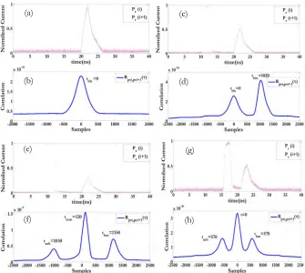
B. CROSS-CORRELATION METHOD (CCM)
in LiDAL systems due to the limited target speed. Further-more, cross-correlation is better than Doppler methods at low speeds, for example to estimate low velocity dispersion using ultrasound signals [57]. Also, cross-correlation has the advan-tage of detecting weak signals [58]. The peak displacement resulting from the cross-correlation between the two snap-shots indicates target movement as the background obstacles are stationary and can also be used to determine target range. In using cross-correlation we firstly look at coarse time scales to determine if there is a mobile target. We refer to this as fast cross-correlation. Here two snapshots are correlated over the full observation time windowT. If target movement is detected, then a finer time scale cross-correlation is car-ried out at the slot level comparing two or more time slots, and carrying out each time a cross-correlation of up to S
snap shots. We refer to this finer cross-cross-correlation as slow cross-correlation. We furthermore define a binary Target Movement Indicator (TMI) whose value is equal to one if the fast or the slow cross-correlations show a change, TMI is equal to zero otherwise. Fig. 13 presents the proposed LiDAL snapshot measurements cube for target movement and shows the values of TMI. In Fig. 13, theyaxis represents time and shows a single time frame of durationT subdivided intoN
time slots. Thezaxis of Fig. 13 represents the TMI values associated with fast cross-correlation when two snapshots are cross-correlated. Finally, thexaxis represents TMI values for each time slot when the slow cross-correlation is evaluated. Note that the values of S indicate the number of snapshots cross-correlated. As can be seen in Fig. 13, the first snapshot measurement (i = 1) is stored until the next measurement (i = 2) is collected. Then a cross-correlation between the two snapshots for the whole time duration T is carried out to determine the TMI (‘0’ and ‘1’) i.e. to determine the ‘fast cross-correlation’. In this case, cross-correlating the (i=1) and (i = 2) snapshots yields TMI=0. If TMI is equal to zero, the fast cross-correlation is continued, to carry out cross-correlation between the current snapshot (i = 2) and the next snapshot (i = 3). However, if TMI is equal to one, multiple cross-correlations are implemented between the
FIGURE 13. LiDAL snapshots measurement cube.
identical time slots of the consecutive snapshots yielding the slow cross-correlation. The slow cross-correlation determines the TMI values associated with each time slots. The value of the TMI associated with slotjis referred to as a weight (wj) which represents change/no change in each time slot.
For example,S = 4 represents cross-correlation between snapshots (i = 1), (i = 2), (i = 3) and (i = 2) and yields a TMI value for each time slot where the TMI values (wj) are
(w1,w2 andw3 = 1;w4,w5 andw6 = 0). The values of
the TMI weights are integrated in the proposed LiDAL sub-optimum receiver to detect and localize the targets as will be discussed in conjunction with Fig. 15.
1) FAST CROSS-CORRELATION
To investigate the performance of the proposed cross-correlation method let us consider (i) a single mobile tar-get with a stationary background obstacle, (ii) no ambiguity (i.e. the minimum distance between the mobile target and the background obstacle is1Ror more) and (iii) white Gaussian noise due to the receiver and ambient noise as discussed in Section III. Here, we analyze the key scenarios of interest and in particular we consider five propositions / scenarios to test the fast cross-correlation method to decide the TMI.
Proposition I: we assume that there is no target in the environment, only (background) an obstacle in the two snapshot measurements (i,i + 1) as can be seen in Fig. 14a. The received signal reflected from the obstacle in the presence of noise in theith snapshot, pri(t), can be
expressed as:
pri(t)=βib t−tbi
+ni(t) (50)
and the received signalpri+1(t)is given as:
pri+1(t)=βi+1b t−tbi+1
+ni+1(t) . (51)
The fast cross-correlation function (Rpri,pri+1) of equa-tions (50) and (51) over the listening timeT is:
Rpri,pri+1(τ)=Rbb(τ)+Rbn(τ)+Rnn(τ) (52) where the term Rbb is an auto-correlation function of the
received signal from the obstacle which is defined as:
Rbb(τ), Z T
−T
βib t−tbi
βi+1b t−tbi+1+τ
dt (53)
andRsn is the cross-correlation of the received signal (from
the obstacle) with noise; andRnnis the noise auto-correlation.
These two correlations are given as:
Rbn(τ), Z T
−T
βib t−tbi
ni+1(t+τ)dt
+ Z T
−T
βi+1b t−tbi+1
ni(t+τ)dt (54)
and
Rnn(τ), Z T
−T
FIGURE 14. Cross-correlation method (a) and (b) received signal and CCM of received snapshots measurement of Proposition I respectively, (c) and (d) received signal and CCM of received snapshots measurement of Proposition II respectively, (e) and (f) received signal and CCM received snapshots measurements of Proposition III respectively and (g) and (h) received signal and CCM received snapshots measurement of Proposition IV respectively.
FIGURE 15. LiDAL receiver block diagram with CCM.
The correlation factorˆt(i.e. displacement factor which
rep-resents the time delay) can be calculated by determiningτ = ˆ
tfor whichRbbis maximized. Therefore,tˆbbis defined as:
ˆ
tbb =arg max
τ (Rbb(τ)) (56)
It should be noted that the noises in the snapshot mea-surements are assumed uncorrelated and orthogonal, thus Rnn≈0 [59], [60]. Also, the value ofRbn can be assumed
very small and can thus be neglected [59], [60]. Hence, Rbb ˆtbb
identifies whether there is a change or not between the snapshot measurements. For proposition I, the obstacle is stationary (tbi = tbi+1∀i). Thereforeˆtbb = 0, see Fig. 14b, indicates that no change took place in the ‘‘target’’ location (TMI=0). Note that the received signal is sampled with
Ts=0.01ns as discussed in Section III-C, which yields thex
![TABLE 1. Reflection model for a different target coating materials [17].](https://thumb-us.123doks.com/thumbv2/123dok_us/1766900.130451/3.576.39.275.63.374/table-reflection-model-different-target-coating-materials.webp)