E rrata for “D isc r e tiz a tio n M e th o d s for C o n tro l S y ste m s
D e s ig n ”
P e r ry A n th o n y B la ck m o re
• pg. 12 (equation 2.2.2): right brace missing after second 7?.(s) • pg. 13 (equation 2.2.3): N over summation should be N
• pg. 14 (last paragraph and henceforth): the notation V(s) G Cnxm is to be understood as the space of functions which map s into the space Cnxm
• pg. 21 (equation 3.2.18): definition is obviously only valid for square systems • pg. 23 (equation 3.2.27): H^(s) should be Hj (z)
• pg. 25 (last equation): g(a) preferable to g(s) • pg. 25 (last paragraph): a T ~ l should be (1 — o,)T_1 • pg. 29 (first sentence): remove “strictly”
• pg. 30 (equation set 3.4.13): these equation naturally apply for all ß such that det(In — ßA) / 0
• pg. 32 (last paragraph): it should be added that, as stated in Chapter 2, the optimization is for a given input signal
• pg. 34 (Lemma 3.5): for consistency of notation we should have
rHz)
(T — a)z z - 1 a• pg. 38 (equation 3.5.30): space missing between equations (between 0 and A T)
• pg. 38 (last two sentences): should read “That is, the sum of the singular values squared is increased. Conversely, as a is decreased, the sum of the singular values squared is decreased.”
• pg. 42 (point 2): We have attempted in this thesis to isolate the factors which affect the magnitude of discretization errors—the Hankel singular values are one of these factors. One of the problems we faced was in trying to vary one of the parameters which affect discretization error, while holding others constant (which also have a relationship to discretization error). Despite this difficulty, the vast amount of simulation work that was undertaken, demonstrated to a large degree that the magnitude of the Hankel singular values significantly influence the magnitude of the discretization errors produced, provided they are viewed in conjunction with other factors. The statement on pg. 95 which states that the factors identified in the open-loop are not so conclusively demonstrable in the closed-loop setting is mainly due to the difficulty in isolating the factors.
• pg. 45 (2 paragraphs following equation 3.6.12): Naturally equation 3.6.12 is not applicable for the e = 0 and e = 1 case. The phenomena in the limiting situation is being addressed in this section.
• pg. 47 (second last equation): dr should be dt
• pg. 52 (Proposition 3.1 and following): The proposition that the discretization process can be modelled as adding a white noise source to each analog integrator clearly has some limitations. Due to the presence of memory, the errors generated are more lowpass in nature. Also a “sufficiently rich” input signal can never be perfectly achieved due to aliasing considerations. However the arguments presented in this section are parallel arguments to those used in the analysis of the propagation of quantization errors in finite wordlength applications. In the analysis of quantization errors, the whiteness assumption is never actually obtained. Despite this, useful practical results can still be obtained. This fact provides the motivation and rationale of the analysis of this section. Simulation results confirm the usefulness of the results obtained.
• pg. 75-77: T~(.z) represents the reciprocal transpose of T(z) and for consistency of notation should be replaced by T~ (z)
• pg. 75-77: n _ [ ] and n+[-] are the stable and antistable projection operators respectively and for consis tency of notation should be replaced ^y [•]_ and [•]+ respectively
• pg. 95 (third paragraph): the 3 occurrences of k should be replaced by N
• pg. 98 (sentence after equation 4.5.8): sentence should read, “The initial degradation...”
• pg. 114 (last sentence before Section 5.3): While objections may be raised against choosing long sampling periods for continuous-time discretization methods, this thesis has attempted to show that good perfor mance can still be possible in this case. Our motivation in selecting long sampling periods was basically twofold. As is well known, good performance can always be obtained (providing numerical problems are not introduced) if the sampling period is low enough. Hence it makes little sense to compare different discretization methods with rapid sampling. Secondly and more importantly, there are applications where a short sampling period is not possible due to limitations in processing power. By still being able to use the continuous method of discretization in these situations, the design is likely to benefit (see arguments in Section 1.2).
• pg. 151 (proof of Lemma 3.10): the occurrences of a should be replaced by cq, and ß by a2
D IS C R E T IZ A T IO N M E T H O D S F O R
C O N T R O L S Y S T E M S D E S IG N
N o te to E x a m in ers
The programs described in Appendix F of the thesis can be obtained via anonymous ftp on faceng.anu.edu.au (id number 150.203.43.3).
The following procedure is required.
1. ’’ftp faceng.anu.edu.au” with the username an on ym ou s, and the password given by your user id.
2. ”cd /p u b ”
3. ’’bin”
4. ’’get perry.tar.Z”
5. ’’mkdir discretization”
6. move perry.tar.Z to discretization
7. ”cd discretization”
8. ”zcat perry.tar.Z | tar xf
If you require any assistance, please feel free to email me at [email protected].
D iscretiza tio n M eth od s for
C ontrol System s D esign
Perry Anthony Blackmore
B.Sc. (University of Melbourne)
Grad. Dip, Ed. (Melbourne College of Advanced Education)
Grad. Dip. Sc. (Australian National University)
April 1995
A thesis submitted for the degree of Doctor of Philosophy
of The Australian National University
Department of Engineering
Faculty of Engineering and Information Technology
S ta te m e n t of O rig in a lity
These doctoral studies were conducted under the supervision of Dr Iven M.Y. Mareels and Prof. Darrell Williamson, with Dr R obert Bitmead acting as advisor.
T he contents of this thesis are the results of original research, performed in cooperation w ith Dr Iven M.Y. Mareels and Prof. Darrell Williamson. Approximately 70% of the work is my own. The research described in this thesis has not been subm itted for any other degree or award in any other university or educational institution.
Sections of this work have been presented at conferences and subm itted to journals, as detailed below.
[1] P.A. Blackmore and I.M.Y Mareels. Convex optimization techniques for analog controller discretization, submitted to IEEE Transactions on Automatic Control in April 1995. [2] P.A. Blackmore, D. Williamson and I.M.Y Mareels. Discrete-time simulation techniques
for continuous-time systems, submitted to Automatica in April 1995:
[3] P.A. Blackmore, D. Williamson and I.M.Y Mareels. Discretization of analog controllers by integral approximation, submitted to International Journal of Control in April 1995. [4] P.A. Blackmore, D. Williamson and I.M.Y Mareels. Signal invariant transformation
techniques for the discretization of analog controllers, submitted to IEEE Transactions on Automatic Control in April 1995.
[5] P.A. Blackmore, I.M.Y. Mareels, and D. Williamson. Survey of closed-loop controller discretization techniques with application to a two-tank apparatus, submitted to Auto matica in April 1995.
[6] P.A. Blackmore and D. Williamson. Optimal discretization of analog controllers, in Pro ceedings of the European Control Conference, pages 1703-1708, Groningen, The Nether lands, 1993.
[7] P.A. Blackmore, I.M.Y. Mareels, and D. Williamson. Signal invariant transformation techniques for the discretization of analog controllers, in Proceedings of the 33rd IEEE
Conference on Decision and Control, pages 249-254, Orlando, Florida, 1994.
[8] P.A. Blackmore and I.M.Y. Mareels. Convex optimization techniques for analog controller discretization, submitted to 3f.th IEEE Conference on Decision and Control in February 1995.
D uring my doctoral studies, I have also worked in areas not directly related to the focus of this thesis. This work is contained in the following papers.
[9] P.A. Blackmore and R.R. Bitmead. Duality between the discrete-time Kalman filter and LQ control law. to appear in IEEE Transactions on Automatic Control, accepted December 1994.
[10] P.A. Blackmore and I.M.Y. Mareels. FIR filter design via convex optimization, to be submitted to IEEE Transactions on Signal Processing
A cknow ledgem ents
I would like to thank my supervisor, Iven Mareels, for his efforts over the last three years. I thank him for his encouragement and guidance which has extended to areas
beyond those pertaining to the academic. Thanks for being a great person. I thank Darrell Williamson for his drive in motivating much of the work of this thesis. I also
thank Michael Green and Robert Bitmead for the help they have given me. A special thanks goes David Clements at the University of New South Wales for providing a great
amount of assistance with the implementational aspects of Chapter 5.
To all the people in the Department of Engineering I thank you for your friendships,
especially the guys in the office. To Werner, I thank you for the endless philosophical debates and the ferocious table tennis battles. To my Christian brothers—’Nuth, Aidan, Jeremy, Bob, and Brenan—I thank you for your encouragement and support.
To Bert and Carole Gibson and many of the members of the Westminster Presbyterian Church I express my gratitude for your ministry, your efforts, and your convictions.
The deepest gratitude goes to my parents. They raised me in manner that encouraged me to think. They gave me an opportunity to make it to this point. I love them both
very much.
Of course to my beloved Kim, thank you for marrying me. Just how do you put up
with my idiosyncrasies?
To the LORD—I now know that you are holy and I am not.
“Holy, holy, holy, is the LORD of hosts: the whole earth is full of his glory.”
A b s tr a c t
Given the widespread use of digital computers in the analysis, design and implemen tation of modern control systems, there exists a need for effective and practical dis cretization methods. Motivated by this need, this thesis develops new discretization
techniques for use in control systems analysis and design, as well as in implementation. Both open-loop and closed-loop methods of discretization are considered. While there
exist other discretization methods that are commonly in use, the analysis of this thesis demonstrates that the new methods enjoy many advantages.
Open-loop methods applicable to control system simulation, filter design and feedfor ward control design are developed. Factors which affect the generation and propagation of discretization errors are identified by analytical, heuristic and experimental argu
ments. An algorithm for open-loop discretization is presented which takes these factors into account. The fundamental idea of this method is the replacement of the analog integrators of a continuous-time system by discrete-time approximations. This is done in such a way as to optimize a given cost function with respect to a given input. The
motivation of this work is to develop accurate discretization methods while limiting the complexity of the resulting discretized system. The work results in a better under standing of the discretization process in the control systems context. Connections are made between discretization and concepts from control systems analysis.
Closed-loop discretization methods are developed for the digital re-design of analog
controllers. Three methods are presented which are based upon the theories of signal invariant transformations, optimal control, and convex optimization. The re-design
methods which are developed exhibit particular advantages over existing methods, and
together form a powerful range of techniques for the designer.
An extensive survey of existing re-design methods found in the literature is undertaken.
Comparisons between these methods and those developed in this thesis are made from
C ontents
Statement of O rig in ality ... i
Acknowledgem ents... iii
A b stra c t v N om enclature... : ... xii
1 In tr o d u ctio n 1 1.1 The Open-Loop Problem ... 2
1.2 The Closed-Loop P ro b le m ... 5
1.3 Thesis S t r u c t u r e ... 7
1.4 Contribution of this Thesis ... 10
2 P ro b lem S ta te m e n t 11 2.1 Intro d u ctio n ... 11
2.2 Open-Loop Problem S ta te m e n t... 11
2.3 Closed-Loop Problem S t a te m e n t... 13
3 O p en -L o o p P ro b le m 16
3.1 Introduction... 16
3.2 Signal Invariant T ran sfo rm atio n s... 17
3.2.1 C o n c e p t... 17
3.2.2 Theory ... 18
3.3 Motivation for the Open-Loop Discretization Schem e... 25
3.4 Problem Form ulation... 28
3.4.1 First Order C a s e ... 28
3.4.2 Second Order C a s e ... 30
3.4.3 Mixed Order C a s e ... 32
3.4.4 The Open-Loop Problem S ta te m e n t... 32
3.5 Special Cases to Gain Insight into the P r o b le m ... 33
3.5.1 Special Case Ä = 0 ... 33
3.5.2 Special Case Ä = A ... 39
3.5.3 Special Case Ä = { a i j ö i j }... 40
3.6 The Effects of Approximation Order on Discretization E r r o r ... 41
3.6.1 Scalar R e s u l t ... 42
3.6.2 Second Order R e s u lt... 43
3.6.3 Comparing Discrete Systems Approach ... 45
3.6.4 Summary of Factors which Affect Discretization E r r o r ... 48
3.6.5 Selection Criteria for the Allocation of Approximation Order . . 50
3.7 The Effects of State Space Structure on Discretization Error 51
3.7.1 An Excursion Into Operational A m plifiers... 51
3.7.2 Optimal State Space Structure for the Minimization of Integrator Noise ... 53
3.8 The Discretization A lg o rith m ... 56
3.9 Simulation R e s u lts ... 59
3.9.1 Examination of the Effects of Bandwidth upon Discretization Error 60
3.9.2 Examination of the Effects of the Hankel Singular Values upon Discretization E r r o r ... 63
3.9.3 Examination of the Effects of State Space Structure upon Dis cretization E r r o r ... : ... 64
3.9.4 Case S t u d y ... 67
3.10 Conclusion ... 69
4 C losed -L oop P ro b lem 70
4.1 Introduction... 70
4.2 H. 2 Optimal Control Method ... 71
4.2.1 Introduction ... 71
4.2.2 Primary Optimization - I2 Minimization of Discretization Error
at an Intersample P o i n t ... 72
4.2.3 Secondary Optimization and Main A lg o rith m ... 80
4.3 Convex Optimization M e th o d ... 86
viii
4.3.2 Problem Formulation ... 87
4.3.3 The Use of “qdes” ... 90
4.3.4 Unstable 7 £ ( s ) ... 92
4.4 Integral Approximation M eth o d ... 93
4.4.1 Introduction ... 93
4.4.2 Problem Formulation ... 94
4.4.3 The A lg o rith m ... 94
4.5 Simulation S tu d i e s ... 95
4.5.1 # 2 Optimal Control M e t h o d ... 96
4.5.2 Convex Optimization M e th o d ...101
4.5.3 Integral Approximation Method ...102
4.6 C onclusions... 106
5 E v a lu a tio n o f C lo sed -L oop M eth o d s 108 5.1 Introduction... 108
5.2 The A p p a r a tu s ... 110
5.2.1 Id e n tifica tio n ...110
5.2.2 Analog Controller D e s i g n ... 112
5.3 Algorithm Descriptions...114
5.3.1 Parameter Selections...118
5.4 R esu lts...120
5.5 A n a ly sis... 132
5.6 C onclusions... 134
6 C on clu sio n s 136 6.1 Overview of T h e s is ... 136
6.1.1 The Open-Loop P r o b l e m ...136
6.1.2 The Closed-Loop P ro b lem ...138
6.2 Further W o r k ...139
A p p en d ic es 141 A F a cto riza tio n T h eo ry 141 B S ta b ility T h eory for S a m p led -D a ta S y ste m s 143 C S a m p led -D a ta F requ en cy R esp o n se M eth o d s 147 D D eriv a tio n o f Error B o u n d s 149 D .l Proof of Lemma 3.9 ...149
D.2 Proof of Lemma 3 .1 0 ...150
D.3 Proof of Lemma 3 .1 1 ...151
F.2 Algorithms of Chapter 4 ... 162
F.3 Algorithms of Chapter 5 ... 164
N o m e n c la tu re
Sets and Spaces
M, C
jg>n x m 0n x m
z+
C°([0,oo),<C")
fields of real and complex numbers
spaces of n x m real and complex constant matrices set of non-negative integers
vector space of piecewise-continuous functions from [0, oo) to C 1 that are bounded on compact subsets of [0, oo) and are continuous from the left at every point except the origin
5 (Z + ,C n ) £ p[0, oo)
space of sequences from Z+ to U 1
Lebesgue space of measurable functions f (t ) from [0, oo) to C71
which have finite L p norm, i.e. | | / | | p = (/0°° \fi{t)\p dt)p < oo
/P(Z+) space of sequences v(fc) from Z + to C71 which have finite
lp norm (definition of lp norm below)
H°° Hardy space, functions bounded and analytic outside the open unit disc
H f complementary part of H°°, bounded and analytic within the unit disc
R H°°, real-rational subspaces of H°° and H respectively
N o ta tio n and Operators
a, a, A
at , a*, a *
scalar, column vector, and matrix respectively
transpose, complex conjugate transpose and pseudo-inverse of a constant matrix A, respectively
tr(A )
I n
0
trace of a n x n matrix
n x n identity matrix arbitrary size zero matrix
d iag (//i,. . . , /in) n x n matrix with diagonal elements ( /ii,. . . , /xn) and all other
A,(A)
?r(A)
U A )
*(A),<n(A)
/(■). F(-)
f(0 , F(-)
elements zero
eigenvalues of a matrix A
number of eigenvalues of A in the open right half-plane number of eigenvalues of A in the open left half-plane range space and null space of a matrix A
scalar functions
vector or matrix values functions
PM,
p«
<5(P)
p - ( z )
P M ] - , [PM )]+
<n(P(ejS))
<f(P(e^)) A I B ] C D
[A,B.C,D] ,
continuous-time and discrete-time transfer function matrices respectively
relative degree of a scalar rational transfer function P; difference between the number of poles and the number of finite zeros the reciprocal transpose (P (z -1 ))T
stable and antistable projection of P(z) respectively i.e. if P(z) G RH°° U R H then P(z) can be written as P(z) - [P(*)]_ 4- [P(z)]+ where [P(^)]_ G P P °°, [P(z)]+ e R H°°
frequency dependent singular values of P(-) maximum Hankel singular value of P(-)
state space realization of a rational transfer matrix P(-) = C (s ln — A )-1 B + D
(also define [A, B, C] = [A, B, C, 0])
D isc r e te -T im e N o rm s (w here defined)
A ( °°
Scalar Sequences \\v\\v = ( lv(k)|p ) 1 < p < oo
\k=o
Vector Sequences
loo = sup \v(k)\ k> 0
E l M l p v ( k ) e S ( Z + , C " )
< i =1 /
where Vi is the i'th component of v(-)
|v||oo = max \\viWoo
l < i < n
A
Transfer Function Matrix ||PH2 —
r2n P r , „ n 1 2
/ £ „ , ( p ( e " ) ) dB
1=1
if P(z) G Cnxm then p = min{m,n}
/ 00 '
tr Y , H k ) h T {k)
V / c = 0 >
where h(k) is the impulse response of P(z)
IIPII00 = sup o (P (eJ0)')
o<0<2?r V '
C h a p te r 1
In trod u ction
A utomatic control has played an important role in the advance of engineering
xi. and science. In our modern society, control systems affect everyone’s life. For instance, in modern houses, the temperature and humidity are automatically regulated for comfortable living; in modern aviation, feedback control systems are employed for safe and comfortable air travel; in industry, control systems increase the efficiency of production; and in defence, automatic control has application in many diverse areas
ranging from missile guidance to vibration control in helicopters.
Feedback control systems can be classified in a variety of ways. One classification
of particular importance to this thesis involves the nature of the signals flowing in the control systems—systems can be classified as continuous-time, discrete-time or
sampled-data. Many control systems occurring in nature are continuous-time—-they have internal signals that evolve continuously in time with control signals that flow in the system continuously without interruption. Many of the human body’s regulatory
systems can be described as continuous-time control systems. Conversely, a discrete
time control systems have signals that evolve discretely in time. Many economic systems can be described in this framework. Systems having both discrete and continuous
signals are called hybrid systems or sampled-data systems. These systems generally arise when analog signals of a continuous-time system are sampled for control purposes,
with the control signals calculated via a digital computer. This type of system is a major
focus of this thesis.
The digital computer has changed the methodology of control systems implementation.
CHAPTER 1. INTRODUCTION
2In the past, continuous-time controllers were the norm in industry. Typically they were
realized electrically—using resistors, capacitors, inductors, and operational amplifiers— or mechanically—using hydraulics and pneumatics. While continuous-time controllers are still used in practice, applications of digital control are becoming more widespread. Digital computers are now widely used in the direct on-line control of processes. This
shift can be attributed to the advances made in microelectronics and digital signal processing in recent decades. Typically, digital controllers are more reliable, cheaper,
more compact, less susceptible to ageing and have improved sensitivity to noise and parameter variations.
The digital computer has also impinged on the techniques of controller design. Many of the classical tools of control systems design—-such as Bode analysis, Nyquist analysis, and root-locus analysis—can be more effectively utilized using the digital computer.
Design techniques which were formally very time consuming can now be rapidly com puted using the digital computer. Many of the burdens of controller design have been eliminated. In short, the digital computer has greatly influenced the theory and practice of control engineering.
Of course the digital computer has limitations and introduces new problems. In the area of controller implementation, limitations in computing speed may introduce unac ceptable time delays. Finite wordlength of the digital processor can lead to problems such as the introduction of unstable limit cycles. In control systems design, inaccuracies in system simulation result from discretization errors and finite wordlength effects.
The goal of the work presented in this thesis is to develop techniques to minimize discretization errors in systems design and controller implementation—in both open-
loop and closed-loop. These problems are now discussed in greater detail.
1.1
T he O pen-Loop P roblem
There are a number of instances in control systems design where a continuous-time
system is discretized in isolation, or more specifically when a block or element is dis cretized without considering the interaction with other elements. In this thesis, this
CHAPTER 1. INTRODUCTION
3F ilter Design: The traditional approach to infinite impulse response (HR) discrete time filter design involves first the design of a continuous-time filter and then transformation into a discrete-time filter (c.f. [62]). There are a number of rea
sons for this approach. For example, the art of continuous-time HR filter design is highly advanced and so it is advantageous to incorporate this approach. Also
many useful continuous-time HR methods have relatively simple closed-form de sign formulae. It is clear that an effective means of discretization is essential for the success of this approach.
Feedforward C ontroller Design: There are examples in control system design where discrete-time elements are designed in isolation—e.g. the design of discrete-time feedforward elements. A typical approach is to first design an acceptable analog element and then perform open-loop discretization.
Sim ulation: A major application of open-loop discretization is the simulation of a system containing analog elements on a digital computer. Obviously, this is inte grally related to control system design. During the design process, the designer is typically concerned with how the given system responds to different inputs—
steps, ramps, and sinusoids for example. As the controller design is refined, a number of simulations may be carried out for for a given controller. As a result, the simulation procedure is carried out many times. The importance of accurate
and effective simulation procedures is clearly seen. In essence, the simulation of continuous-time dynamical systems generally requires the numerical solution of a set of differential equations. Discretization or approximation is a feature of these
techniques.
For the discretization of linear, time-invariant dynamical systems where a transfer function description of the system exists, one can think of the discretization process as
transforming a continuous-time transfer function into a discrete-time one. Naturally, there is no unique equivalence between continuous-time and discrete-time systems for
all input signals—with any discretization method there is a loss of information. As a result of discretization, errors are generated and propagated—a natural concern is to
minimize these errors. Before deciding on a particular method of discretization, the designer must decide which properties of the continuous-time system are important to
preserve. There is a wide range of possible frequency-domain or time-domain properties. Furthermore, the complexity of the discretization method is important. Discretization
methods which produce systems of order ten times that of the continuous prototype
CHAPTER 1. INTRODUCTION 4
There exists a large body of literature dealing with discretizing continuous-time systems and in particular, simulating continuous-time systems on a digital computer. Some of the early methods are:
P icard’s m ethod, which generates a series of functions which converge to the true solution. This method is of theoretical interest, and is really only of practical value when an analytic solution is available. Alternative methods are obviously
preferable.
Taylor series m ethods, which apply a recursion formula to generate a series of solution points to the differential equation. This is a good method when analytic expressions for the high order derivatives are known.
R u n ge-K u tta m ethods, which are derived from the Taylor series methods. Runge- K utta methods are widely used, having many advantages of the Taylor series methods, but avoiding the problems inherent with computing high order deriva
tives.
P redictor-corrector m ethods, which are a family of methods involving a pair of formulae, the predictor and the corrector. These methods enable tight control over the error at each point by the repeated application of the corrector and the computation times are generally shorter than those of the Runge-Kutta methods. A disadvantage of the predictor-corrector methods is that they are dependent
upon another method to generate a set of starting values.
Many texts are available which discuss the above methods, see for example [44].
In the survey paper of Kowalczuk [50], two broad classes of open-loop discretization methods are identified. The most popular are the closed-form transform ations,
in which the discretizing transformation is chosen to minimize the difference between the response of the digital model and the the response of the analog prototype at the
sampling points {4 = fcT, k an integer}. The error depends on the input signal
applied. As a result, distinctions are made according to whether the spectrum of the input signal is bandlimited to the Nyquist range (u) : u> < = 7r/T ) or not.
Closed-form approximations can be further divided into direct transform ations and
CHAPTER 1. INTRODUCTION 5
79, 81], and convolution approximation methods [78, 80]. A feature of direct trans formation methods is that the prototype system T{s) is treated as a whole, and an
attem pt is made to preserve the input-output relationship. The indirect approach in volves treating T( s ) as a number of sub-systems such as integrators or differentiators.
These sub-systems are replaced by discrete-time operators. Examples of indirect trans formations include mapping of differentials [42, 62, 82, 84], forward and backward Euler approximations [42, 62, 69, 82, 84], bilinear transformations [11, 42, 62, 64, 76, 82, 84],
and matched ^-transforms [42, 62, 84].
The second broad class of discretization methods can be referred to as open-form approxim ations [4, 35, 62, 63, 64, 70]. These methods generally involve some form of iterative optimization algorithm and do not result in closed form solutions. Most of these methods use a frequency based criterion and are quite often computationally expensive. In engineering, perhaps the most well-known of these methods is that devel
oped by Deczky [24, 62, 63], in which an Lp frequency-domain criterion is minimized.
In this thesis, a unified theory is presented which addresses essential aspects of the
open-loop discretization procedure. Unlike many discretization schemes presented in the literature, the procedure developed attem pts to first determine the magnitude of the expected discretization errors, and then discretize with an appropriate complexity.
The proposed algorithm gives the designer control over the order of the discrete-time system. This enables the design of filters with low complexity which still retain essential
properties of the prototype system.
Attempts are made, where possible, to examine the discretization process from an engineering perspective. For example, a number of relationships are found between the
bound on the magnitude of the discretization error and the Hankel singular values. To our knowledge, this approach is a new contribution.
1.2
T he C losed-Loop P roblem
The design and implementation of sampled-data controllers motivates the study of
minimizing discretization error in a closed-loop setting. Of course there are many practical issues in the design of sampled-data controllers—the design of the digital-
C H A P T E R 1. IN T R O D U C T IO N 6
the com puter is the focus in this thesis.
Discretize Plant
Discretize Controller
Direct Approach
Discrete-Time Controller Design Continuous-Time
Controller Design
Figure 1-1: Methods of sampled-data controller design
Figure 1-1 represents the three choices of sam pled-data design method. These are:
D isc r e tiz e P la n t A pproach: The given model of the continuous-time plant is re placed by an equivalent discrete-time model. A discrete-time design m ethod (such as those found in [6, 32]) is then used to generate a discrete-time controller. There are two main disadvantages with this approach. First, a priori decisions such as the choice of sampling-rate and possible sampling-skew must be made. But sensible choices of these quantities depend upon the performance of the fi nal closed-loop system. If these quantities are not estim ated correctly, the whole design may have to be repeated. A second problem of this approach is th a t in tersam ple behaviour is ignored at the start of the design. For this reason, the resulting performance of the digital controller may be poor.
D isc r e tiz e C on troller A pproach: A continuous-time controller may be designed based on the continuous-time plant. The continuous-time controller can then be discretized using a number of different methods. Controller discretization m ethods can be found in [1, 32, 43, 45, 50, 52, 53, 54, 58, 60, 61, 65, 66, 67, 71, 85]. This approach is favourable if the designer is more familiar with continuous-time design. Loop shaping problems and constraint satisfaction can be achieved more effectively than with direct methods. Additionally, in contrast to the “Discretize P lant Approach” , this approach allows intersample behaviour to be taken into account in the design.
CHAPTER 1. INTRODUCTION 7
18, 19, 20, 21, 26, 38, 40, 41, 46, 73, 74, 75, 86]. In particular, the sampled-data
H2 problem has been tackled by Khargonekar and Sivashankar [46], Bamieh and Pearson [9], Chen and Francis [18, 20] and Chen [17]. The sampled-data H0Q
problem has been addressed by Toivonen [75], Bamieh and Pearson [10], and
Kabamba and Hara [41]. Dullerud and Francis have developed theory for the L\
sampled-data problem. Despite the mathematical difficulties present in describing
sampled-data systems, the above work represents a significant advance. However, the calculations are generally very forbidding. Experience indicates that these methods do not allow the designer a great deal of flexibility—there are many
situations in which a better design can be achieved by “indirect” approaches, particularly if the designer has more experience in the area of continuous-time controller design or if there are multiple control objectives. These approaches are also difficult to apply to complex systems. Furthermore, the H2 sampled-data
approach often yields digital controllers that generate large control signals. This can be a problem in practical settings.
There are many situations in which the “Discretize Controller Approach” is preferable, producing a superior performance to the “Direct Approach” . It is therefore important that effective controller discretization schemes exist. This thesis presents optimization
based controller discretization algorithms which are shown to produce sampled-data controllers with excellent performance. The algorithms developed are shown to have
many advantages over other discretization schemes presented in the literature.
1.3
T h esis Structure
A brief outline of the progression of ideas in this thesis is as follows:
Signal Invariant Transformations
After the problems addressed in this thesis are formulated at a conceptual level in
Chapter 2, the introductory material of Chapter 3 presents a review of the existing theory of signal invariant transformations. This material is foundational for much of
the theory presented in this thesis. The signal invariant transformation, for a particular input signal, allows a continuous-time system to be discretized so that the sampled output of the continuous-time system is equivalent to the output of the discrete-time
CHAPTER 1. INTRODUCTION 8
continuous-time system has an order typically equal to the order of the continuous time prototype plus the order of the continuous-time model whose impulse response generates the input signal.
D isc r e tiz a tio n v ia In tegral A p p ro xim a tio n
The open-loop discretization method is introduced in Sections 3.3 and 3.4. The basis of
the scheme is a modification of the Newton-Cotes formulae for numerical integration. Each integrator of an n-dimensional system is replaced by a Newton-Cotes type ap proximation. The order of the approximation of each integrator may vary. The method
is an open-form approximation technique using iterative optimization. A time-domain criterion is used with a formulation in terms of state space structures. Optimization
is performed with respect to a given signal. This method gives a lower order discrete time system than the signal invariant transformation technique without a severe loss of time-domain performance.
Factors which affect discretization error are then identified. These factors are incorpo
rated into the discretization methodology and a unified theory is presented. An analysis of the effects of state space structure is given and theory is presented which enables the selection of state space structures favourable for minimizing discretization error.
C on troller D isc r e tiz a tio n U sin g H2 O p tim al C on trol T h eo ry
Chapter 4 presents the closed-loop discretization methods. Existing literature ap
proaches this problem in basically two ways:
1. Open-loop analog-to-digital conversions using, for example, the bilinear, forward
difference, backward difference, step invariant and impulse invariant transforma
tions [6, 42, 84].
2. Closed-loop analog-to-digital design using signal invariant transformations [84] or
other techniques [1, 43, 45, 65].
It is now well recognised that, when designing a digital controller to replace an analog controller, the closed-loop properties of the continuous-time system (consisting of ana
log controller and plant) should be taken into consideration. Consequently, closed-loop
CHAPTER 1. INTRODUCTION
9rate by a factor of 10 in comparison to the open-loop approaches. With this motiva
tion, this thesis presents three methods of closed-loop controller discretization. The first method, found in Section 4.2, uses an extension of the open-loop signal invariant transformation theory. Optimal control theory is used and a number of algorithms are
proposed. The method is shown to perform favourably when compared with existing algorithms. A disadvantage of this method is that digital controllers of high order are produced. The sampled-data controller reduction method of [56] is shown to effectively deal with this problem.
C on troller D iscretiza tio n U sin g C onvex O p tim iza tio n T echniques
In Section 4.3, a similar problem is solved using signal invariant transformations and convex optimization techniques. This theory is based on the work of [13]. The convex
optimization technique is shown to be an extremely powerful method of design. A variety of constraints can be incorporated into the design which makes this the most flexible method of controller discretization available. Again the disadvantage of this
method is that the resulting digital controllers are of high order.
C o n tro ller D isc r e tiz a tio n U sin g In tegral A p p rox im a tio n s
The open-loop discretization method developed in Chapter 3 is extended to the closed- loop setting in Section 4.4. Although a non-linear optimization problem results, this method has the advantage that model order reduction techniques are not required in the final phase of design. Unfortunately the method suffers from the existence of local
minima. However a simple technique which greatly alleviates the numerical difficulties associated with this problem is presented.
C om p arison o f D isc r e tiz a tio n M eth o d s
The controller discretization algorithms developed in this thesis are then compared to existing methods presented in the literature. The comparison involves a short simu
lation study in Section 4.5 and an extensive analysis in Chapter 5. The analysis in
Chapter 5 is based on computer simulations, practical experimentation and subjective analysis. The three methods developed in this thesis are demonstrated to be extremely
CHAPTER 1. INTRODUCTION 10
1.4
C ontribution of this Thesis
The preceeding discussion demonstrates a four-fold contribution of this thesis:
O p en -L oop D iscretiza tio n M eth od
• comprehensive treatment of the open-loop discretization problem
• theory for replacing the integrators of a continuous-time system by discrete
time approximants, which allows the designer to control the complexity of the discretization
• techniques wrhich enable the designer to identify the factors which affect discretization error
• theory which gives good state space structures for discretization
C losed -L oop D iscretiza tio n M eth o d s
• discretization method using signal invariant transformations and optimal control theory
• discretization method based on signal invariant transformations and convex optimization
• discretization method based on integral approximations
S u rvey o f D isc r e tiz a tio n M eth o d s
• comprehensive survey of closed-loop discretization methods
A lg o rith m s
• open-loop discretization—includes algorithms for parameter optimization
and optimization of state space structure for discretization
• controller discretization using H2 optimal control theory
• controller discretization using convex optimization
• controller discretization based on integral approximations
C hapter 2
P rob lem Statem en t
2.1
Introduction
A s stated in Chapter 1, the primary focus of this thesis is to develop discretization 1 techniques for use in the open-loop and closed-loop settings. This chapter refines
this statement by presenting formal problem statements for both problems. The prob lems are formulated at a conceptual level at this point, and are further elaborated and refined in Chapters 3 and 4.
2.2
O pen-Loop P roblem Statem ent
The discretization problems considered in this thesis are restricted to linear, finite dimensional systems. A continuous-time system can be viewed as a mapping from
C°([0,oo),Cn ) -» C°([0,oo),Cn ), whereas a discrete-time system can be viewed as a
mapping from <S(Z+, C 1) -» <S(Z+, C 1). The general problem of discretization is finding a transformation X) which maps a given continuous-time system Q(s) into a discrete
time system G(z), i.e.
G(z) =3) ( f f ( 5) ) (2.2.1)
Ideally the transformation would be such that the responses of both systems would be identical (at the sampling instances) for any input signal, not necessarily piecewise
constant. However this is not possible in reality when realizability and complexity
CHAPTER 2. PROBLEM STATEMENT 12
issues are encountered. Only some of the properties of Q{s) can be preserved under the D-transformation. Therefore, the discretization problem can be thought of as finding
a X) which minimizes
& { $ ( * ) - G ( * ) }
for some distance function 5 0.
Assume that the continuous-time system Q(s) is driven by a signal r(£) for t > 0.
Assume also that the discrete-time system is driven by the sampled r(t) which is denoted by S ^ r(t). The sampling operator (with period T) is defined in Appendix B.
Let the continuous-time input signal r(t) be generated by the impulse response of a strictly proper system 7£(s). With a slight abuse of notation, let the sampled r(t) be represented by Sx7Z(s). Similarly, let the sampled output of Q(s) be represented by
S tQ(s)71(s).
The minimization of
2o{St£ ( 5 W S) - G(z)StK (s)}
is sought for some distance function $0 which is now defined.
Let Q{s) represent a strictly proper, linear time-invariant system. Let 7Z(s) represent a strictly proper, linear time-invariant reference model whose impulse response is r (£), t >
0. Let the response of Q(s) (with zero initial conditions) to r(t) be represented by
y(t), t > 0. Furthermore, suppose y (kT) is the sampled values of y(t) at t — k T with
k = 0 , 1 , . . . , oo for some sampling period T > 0. Similarly, let r{kT) be the sampled r (t) for k = 0 ,1 ,..., oo. Let G(z) be restricted to the class of linear, time-invariant
systems. Finally let y( kT) be the response of G(z) (with zero initial conditions) to
r (kT).
Define the distance function $ 0 to take the form of a cost function Jn where
N
50{S TS(s)H(s) - G (z)StK (s) = J N = ||y (kT) - y ( k T ) f 2 (2.2.2)
k= 0
This cost function is chosen for several reasons. It gives a good measure of error between
the continuous-time and discrete-time systems. It is computationally easy to calculate.
By varying N, the discretization error during the transient response (by making N T
small) or the steady-state (by making N T large) can be targeted. As N —> oo, with T
fixed, J N is the I2 norm—in this case Parseval’s theorem indicates that Jn is related
to the frequency-domain error.
A transformation X) is sought to minimize (2.2.2) subject to the realizability of G(z).
CHAPTER 2. PROBLEM STATEM EN T 13
of G(^). Therefore a parameterization of G(z) is established so that restrictions on the complexity of G(z) are managed. Represent this parameterization as G(z, p) for some parameter p. Define y p(kT) to be the response of G(z, p) (with zero initial conditions) to r(kT).
The open-loop problem addressed by this thesis is to
find a parameter p which achieves the minimization
minjyv(p)
p where
N
Jn(p) =
E
lly(fcT) - yp (* T )f2 (2.2.3) A:=0with
y (t) =
y(kT) = G(z, p)r(kT)
The choice of parameterization is presented in Chapter 3.
2.3
C losed-Loop P roblem Statem ent
The general aim of digital re-design is to replace an analog controller C(s) by a dig
ital controller C fiz ) so that the performance of the closed-loop sampled-data system ‘approximates’ the performance of the closed-loop analog system. The addition of a
discrete element in an analog environment requires that there is a process of signal conversion so that the digital and analog components can be interfaced in the same
system. Therefore analog-to-digital converters, digital-to-analog converters, sample- and-hold devices and multiplexers are inherent in the overall design. Naturally there
are complex issues associated with the design and implementation of these components.
However the following assumptions are made in this thesis:
• The analog-to-digital converters have infinite wordlength.
• The digital-to-analog converters are ideal: that is, there is zero acquisition time, zero aperture time, zero settling time and zero hold-mode droop.
• The hold function is a zero order hold. Although the theory of this thesis does not
CHAPTER 2. PROBLEM STATEMENT
14Analog Feedback Control System
r(t)
o
e(t)C(s) u(t) P(S) y(t)
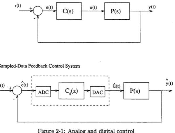
Sampled-Data Feedback Control System
Figure 2-1: Analog and digital control
in practical applications.
These assumptions are common to most discretization methods and are reasonable for most applications.
Anti-aliasing filters are also a common addition in the re-design process. These are generally analog devices placed before the samplers. They do not appear explicitly in the re-design theory of this thesis. However if the dynamics of these filters have
a significant effect on the overall system dynamics, they can be readily accounted for with the theory developed.
In Figure 2-1, an analog unity feedback control system is illustrated. The system consists of a strictly proper, linear time-invariant plant V{s) G Cnxm and a proper
linear-time invariant controller C(s) G Cmxn. Assume also a strictly proper linear
time-invariant reference model 7£(s) G Cn x l, whose impulse response generates the reference signal r(£). The output of the analog closed-loop system is represented as
y(t). The sampled-data unity feedback control system shows the digital controller
Cd{z) with analog-to-digital converter and digital-to-analog converter. The output of
[image:31.519.119.419.123.351.2]CH APTER 2. PROBLEM STATEM ENT 15
A ssu m p tio n s: Suppose the analog controller C(s) has been chosen such that:
A The closed-loop system is asymptotically stable.
B The output tracking error ||y(£) - r(t)|| -> 0 as t -» oo where r(t) = £ -1 {7£(s)}
is the impulse response of the reference model H(s).
Let the plant, continuous-time controller, and reference model be considered as oper
ators, mapping C°([0, oo), Cn ) -» C°([0, oo), Cn )—denote these operators as simply V, C and H respectively.
The closed-loop operator of the analog closed-loop system is given by
n :C°([0,oo),Cn ) ->C°([0,o o ),e n ) where H = V C (ln + T C ) ~ X (2.3.1)
The digital controller is an operator mapping 5 (Z +,C n) —>• S ( Z +,C n).
The closed-loop operator of the sampled-data closed-loop system is given by
Sir = -PHtCjStCIu + (2.3.2)
where the sampling operator St, and the zero-order hold operator H7- are defined in
Appendix B. The operator Sj t maps C°([0, 00), Cn ) —> C°([0, 00), Cn ).
The closed-loop problem addressed by this thesis is to find a stabilizing digital controller Cd{z) which minimizes
ZcI &t - ' H ) ' * } (2.3.3)
for some distance function $ c.
The operator $ c is algorithm dependent. Stability in this sense means exponential sta bility; input-output stability is not addressed by the algorithms developed. Appendix
B contains a discussion of stability of sampled-data systems. For a detailed treatment,
see [19, 29].
The closed-loop problem can be alternatively stated: find a stabilizing digital controller
Cd{z), such that
$ c { y { t )
- yW}
C h a p te r 3
O p e n -L o o p P ro b le m
3.1
Introduction
rTTI his chapter presents a comprehensive treatment of the open-loop discretization
JL
problem. As stated in Chapter 1, the general aim of the discretization method developed in this thesis is to give the designer control over the complexity of the dis cretization. This is achieved by first identifying the factors which influence the mag nitude of the discretization error and then adjusting the complexity accordingly. Forexample, if a large sampling period is used which is conducive to large errors, then a complex discretization method may be warranted.
In this chapter, the signal invariant transformation is used as the benchmark of open-
loop discretization performance. It is also used extensively in the closed-loop techniques of Chapter 4. Because of its important role , this chapter presents a detailed treatment
of signal invariant transformations. As mentioned in Chapter 1, this transformation
allows a discretization which gives perfect matching in response to a reference signal. If ni is the order of the analog system and 772 is the order of the model that generates
the input signal, then the order of the discrete system produced by a signal invariant
transformation is typically equal to 77,1 +772- This complexity may be detrimental to performance in some applications, for example in an environment where there are restrictions on the computational time. A lower order discretization is generally sought
in such cases. A fundamental concern of this chapter is finding a discretized system of lower order (if one exists) which allows “near perfect” matching.
CHAPTER 3. OPEN-LOOP PROBLEM 17
The particular parameterization used in the open-loop discretization method is based on a Newton-Cotes method of integral approximation. In an n-dimensional continuous
time system there are n integrators. The discretization method replaces each of these integrators by a modified Newton-Cotes discrete-time approximation, parameterized by a vector p. The parameterization allows the designer to control the complexity of
the discretization by allowing each analog integrator to be replaced by either a zeroth, first, or second order digital approximation. An optimization is then performed to find
a p which minimizes the open-loop cost function (2.2.3), introduced in Chapter 2. The discretization problem is formulated in terms of a state space description.
A major emphasis of this chapter is to identify the factors which contribute to and affect the magnitude of discretization errors. These factors are identified by analytical, heuristic and experimental means. As mentioned in Chapter 1, these factors are linked to concepts found in control theory, such as the Hankel singular values. The effect of
state space structure on the generation and propagation of discretization errors is also investigated in this chapter.
This chapter is organized as follows. Section 3.2 presents the theory of signal invariant transformations. A motivation of the open-loop discretization scheme is given in Section 3.3. The open-loop problem that is initially formulated in Chapter 2 is fully formulated in Section 3.4. A number of special cases are looked at in Section 3.5 in order to gain an
insight into the parameterization used. By looking at the effects of approximation order on discretization error, the factors which affect discretization error are then identified in Section 3.6. The effects of state space structure on discretization error are identified
in Section 3.7 and an algorithm which givens an “optimal” state space structure is presented. A summary of results appears in Section 3.8 and the discretization algorithm
is presented. Simulation results are presented in Section 3.9, with conclusions drawn
in Section 3.10.
3.2
Signal Invariant Transformations
3 .2 .1 C o n c e p t
Figure 3-1 gives a diagrammatic representation of the signal invariant transformation. A continuous-time system G(s) with a continuous-time input and output is shown.
CHAPTER 3. OPEN-LOOP PROBLEM 18
Figure 3-1: Representation of the signal invariant transformation
input signal if the sampled input applied to Gd(z) yields an output equivalent to the sampled output of G(s). This relationship is shown in the figure.
3 .2 .2 T h e o r y
Consider a continuous-time transfer function matrix 'H(s) having a minimal state space
representation
« ( s ) = C 1(äI„l - A 1)_1B 1 (3.2.1)
In the special case where 9i(s) is single input, single output (SISO), the transfer func
tion is denoted by
H(s) = c f ( s l ni - A i ) -1bi
The impulse response, h(t), with respect to an impulse at time 0, is given by
m = crl{U(a)}
C 1eAltB 1 t > 00 t < 0 (3.2.2)
where C denotes the Laplace transform operator. The z-transform Ht{z) of the uni formly sampled values {h(fcT); k non-negative integer} of h(t) is given by
Ht(2) = Z{CieAl*TB i} = zC!
( a ni
- F i ) _1Bi ; F, = eAlT (3.2.3)D e fin it io n 3.1 The discrete-time system Ht(z) in (3.2.3) is said to be the impulse invariant transformation of'H(s), and is written
CH APTER 3. OPEN-LOOP PROBLEM 19
The subscript T is used to explicitly indicate th a t Ht{z) depends on the sampling period T.
L em m a 3.1 (i) The impulse invariant transform Ht(z) oP H (s) in (3.2.1) is a proper discrete transfer function given by
Ht(z) = Q B j + CM zIn, - F 1) - ‘F 1B i ; F , = eA ' T (3.2.5)
(ii) Ht(z) is strictly proper if and only if C1B1 = 0 .
(Hi) For C1B1 ^ 0 , the Smith zeros o f Ht(z) are given by the eigenvalues of
In the SISO case, there are n\ zeros o f Ht{z).
(iv) In the SISO case, if c f b i = 0, then His) has relative degree o f at least 2, but
Ht(z) has relative degree 1 for almost every sampling period T.
P ro o f: P arts (i)-(iii) follow by expansion of (3.2.3). Now suppose c f b i = 0. Then
Ht(z) is of relative degree 1 if and only if c ^ F ib i ^ 0. But F i (see (3.2.5)) is an analytic function of T, and so c f F i b i does not vanish for almost every T. This proves p art (iv).
The z-transform Ht^ (z) of the uniformly sampled values { h( kT + £); k non-negative integer, 0 < £ < T} of h(t) is given by
H Tl€W = Zt s{ H( 8 ) } (3.2.6)
= 2 { C ,e Al(,!r+?)B 1} (3.2.7)
= C ie A‘{B ! + C 1eAl«(zI„1 - F O - 'F i B j ; F , = eA' T (3.2.8) Note th a t H ^ ^(z) is proper, but not strictly proper, for almost all values of T and £.
D e fin itio n 3 .2 The discrete-time system Ht,z(z) in (3.2.6)-(3.2.8) is said to be the £-offset impulse invariant transformation of Hi s), and is written
C H APTER 3. OPEN-LOOP PROBLEM 20
Some properties of the impulse invariant transformation of cascaded systems are now
examined. Suppose
UG(s)=- H( s) Q(s) (3.2.10)
where the strictly proper K (s) is given by (3.2.1), and the proper system C?(s) has a
minimal state space representation
S(s) = D 2 + C 2(sI„2 - A 2)_1B 2 (3.2.11)
Then a state space representation of 'HG(s) is given by
H 6 ( s ) = U(s)D 2 + C (sI„,+ „2 - A ) - 'B (3.2.12)
where
; C = [ C i 0 ] (3.2.13)
In the SISO case, the representation of LiQ(s) in (3.2.12) is minimal if and only if there are no pole-zero cancellations between 'H(s) and Q(s).
L e m m a 3.2 The impulse invariant transformation H G 'r(z) of'HG(s), when 'H(s)
and Q(s) have different poles, deßned by (3.2.12) and (3.2.13) is given by
H G T (z) = Ht(z)D 2 + H G i(z) (3.2.14)
where
H G iW = C i(2 lBl - + (zl„2 - FjJ -'FjIBs
where Ht(z) is given by (3.2.5), and where the m x n 2 matrix F i2 is given in terms o f
an rt\ x n 2 matrix P i 2 by
Fi2 = P i 2F 2 - F 1Pi2 (3.2.15)
Pi2A 2 — AiPi2 = BiC2 (3.2.16)
In particular, when D 2 = 0, H G ^(z) is strictly proper.
P ro o f: Define the (nx + n2) x (ni + n2) similarity transformation
0 Iri2 Ai B i C ,
o a2 B
0
CHAPTER 3. OPEN-LOOP PROBLEM 21
where P i 2 is defined by the equation (3.2.16). From the theory of Sylvester equations (see [7] for example), P i 2 is uniquely defined because by assumption A i and A 2 have different spectra. From (3.2.13)
P _1A P = Al ° 0 A 2
Moreover, from (3.2.13), CB = 0 and so from Lemma 3.1
H G T(z) = H T(z)D2 + C (z lni+n2 - F ) - 1FB ; F = eAT
Then
A P T n - l Fi
0 F l 2
f2
F 2 £ eA*T
where F i and F i2 are given by (3.2.3) and (3.2.15) respectively, which then gives (3.2.14). When D 2 = 0, H G (z) is strictly proper. |
A similar result can be derived for the ^-offset impulse invariant transformation H G ^ ( 2 )
of 'HQ(s). Note that even when D 2 = 0, H G ^ ^ z ) is almost always proper and not
strictly proper for f 7^ 0.
D e fin itio n 3.3 Consider a signal v(t) = C 1{V(s)}. Then the discrete-time system
Ht(z) written
H vT (z) = Z^ { U( s ) } (3.2.17)
where
ZvT { n ( s ) } = Zt{ H (s)V (s)}[Z rlV fs)}]“ 1 (3.2.18)
is said to be the signal invariant transformation of'H(s) in (3.2.1) with respect to v(t).
The subscript T and superscript v on the operation Zj.{-} in (3.2.17), (3.2.18) indicate that a signal invariant transformation depends explicitly on both the sampling period T
and the reference signal v(£). The relationship in (3.2.18) says that the continuous-time convolution of v(t) with h(t) in (3.2.2), followed by sampling, is equal to the discrete time convolution of the sampled values {v(A:T)} with the sampled values (h(/cT)}. In the general multivariable setting, a restriction applies on the signal model V(s) to
CHAPTER 3. OPEN-LOOP PROBLEM 22
V(s) = [A2.B 2,C ‘2]. It will be shown shortly that in the SISO case, this condition is
not required.
By a slight abuse of the definition, H ^(z) in (3.2.3) was called an impulse invariant transformation. However there is actually no signal v(t) such that
V(s) = £{v (i)} = I„2 ; ZT {V{s)} = Z{ v ( k T) } =I„2
D e f i n i t i o n 3.4 Consider a signal v(t) = C 1{V(s)}. Then the discrete-time system
written
H VT ^ (z ) = z ^ { H ( s ) } (3.2.19)
where
Z ^ m s ) } = ZTA{ U(s)V( s) } [Zt{V(s)}]-1 (3.2.20)
is said to be the ^-offset signal invariant transformation of'H(s) in (3.2.1) with respect to v(i).
E x a m p le 3.1: A state space realization of the ^-offset step invariant transformation of EL(s) in (3.2.1) is given by
r T r t
,Ai T, / eAlTB 1dr, CieAl^,Ci [ eAlTBx dr
Jo Jo (3.2.21)
To conclude this treatment of signal invariant transformations, some results for SISO systems are presented.
C o r o l l ar y 3.1 (i) Suppose
V(s) = 1
s + a
and H{s) = c j (s lni — Ai) has no poles at s = —a. Then
tfKz) = cf(zIn1 - F , ) - 1f 12
where
fi2 = ( F 1 - e - ° 7'lni) (A1 + a I „ 1) - 1b 1 ; F, =
(3.2.22)
In particular, when 'H(s) has no poles at s = 0, the step invariant transformation H ^(z)
(corresponding to a = 0) is given by