A new multistage lattice vector quantization with adaptive subband thresholding for image compression

Volume 2007, Article ID 92928,11pages doi:10.1155/2007/92928

Research Article

A New Multistage Lattice Vector Quantization with Adaptive

Subband Thresholding for Image Compression

M. F. M. Salleh and J. Soraghan

Institute for Signal Processing and Communications, Department of Electronic and Electrical Engineering, University of Strathclyde, Royal College Building, Glasgow G1 1XW, UK

Received 22 December 2005; Revised 2 December 2006; Accepted 2 February 2007

Recommended by Liang-Gee Chen

Lattice vector quantization (LVQ) reduces coding complexity and computation due to its regular structure. A new multistage LVQ (MLVQ) using an adaptive subband thresholding technique is presented and applied to image compression. The technique con-centrates on reducing the quantization error of the quantized vectors by “blowing out” the residual quantization errors with an LVQ scale factor. The significant coefficients of each subband are identified using an optimum adaptive thresholding scheme for each subband. A variable length coding procedure using Golomb codes is used to compress the codebook index which produces a very efficient and fast technique for entropy coding. Experimental results using the MLVQ are shown to be significantly better than JPEG 2000 and the recent VQ techniques for various test images.

Copyright © 2007 M. F. M. Salleh and J. Soraghan. This is an open access article distributed under the Creative Commons Attribution License, which permits unrestricted use, distribution, and reproduction in any medium, provided the original work is properly cited.

1. INTRODUCTION

Recently there have been significant efforts in producing ef-ficient image coding algorithms based on the wavelet trans-form and vector quantization (VQ) [1–4]. In [4], a review of some of image compression schemes that use vector quan-tization and wavelet transform is given. In [1] a still image compression scheme introduces an adaptive VQ technique. The high frequency subbands coefficients are coded using a technique called multiresolution adaptive vector quanti-zation (MRAVQ). The VQ scheme uses the LBG algorithm wherein the codebook is constructed adaptively from the in-put data. The MRAVQ uses a bit allocation technique based on marginal analysis, and also incorporates the human visual system properties. MRAVQ technique has been extended to video coding in [5] to form the adaptive joint subband vec-tor quantization (AJVQ). Using the LBG algorithm results in high computation demands and encoding complexity partic-ularly as the vector dimension and bit rate increase [6]. The lattice vector quantization (LVQ) offers substantial reduction in computational load and design complexity due to the lat-tice regular structure [7]. The LVQ has been used in many image coding applications [2,3,6]. In [2] a multistage resid-ual vector quantization based on [8] is used along with LVQ

that produced results that are comparable to JPEG 2000 [9] at low bit rates.

Image compression schemes that use plain lattice VQ have been presented in [3,6]. In order to improve perfor-mance, the concept of zerotreeprediction as in EZW [10] or SPHIT [11] is incorporated to the coding scheme as pre-sented in [12]. In this work the authors introduce a technique called vector-SPHIT (VSPHIT) that groups the wavelet coef-ficients to form vectors before usingzerotreeprediction. In addition, the significant coefficients are quantized using the voronoi lattice VQ (VLVQ) that reduces computational load. Besides scanning the individual wavelet coefficients based on zerotreeconcept, scanning blocks of the wavelet coefficients has recently become popular. Such work is presented in [13] called the “set-partitioning embedded block” (SPECK). The work exploits the energy cluster of a block within the sub-band and the significant coefficients are coded using a sim-ple scalar quantization. The work in [14] uses VQ to code the significant coefficients for SPECK called the vector SPECK (VSPECK) which improves the performance.

quadtree modelling process of the significant data location. The threshold setting is an important entity in searching for the significant vectors in the subbands. Image subbands at different levels of decomposition carry different degrees of information. For general images, lower frequency subbands carry more significant data than higher frequency subbands [15]. Therefore there is a need to optimize the threshold values for each subband. A second level of compression is achieved by quantizing the significant vectors.

Entropy coding or lossless coding is traditionally the last stage in an image compression scheme. The run-length cod-ing technique is very popular choice for lossless codcod-ing. Ref-erence [16] reports an efficient entropy coding technique for sequences with significant runs of zeros. The scheme is used on test data compression for a system-on-a-chip design. The scheme incorporates variable run-length cod-ing and Golomb codes [17] which provide a unique binary representation for run-length integer symbol with different lengths. It also offers a fast decoding algorithm as reported in [18].

In this paper, a new technique for searching the signif-icant subband coefficients based on an adaptive threshold-ing scheme is presented. A new multistage LVQ (MLVQ) procedure is developed that effectively reduces the quantiza-tion errors of the quantized significant data. This is achieved as a result of having a few quantizers in series in the en-coding algorithm. The first quantizer output represents the quantized vectors and the remaining quantizers deal with the quantization errors. For stage 2 and above the quan-tization errors are “blown out” using an LVQ scale factor. This allows the LVQ to be used more efficiently. This differs from [2] wherein the quantization errors are quantized un-til the residual quantization errors converge to zero. Finally the variable length coding with the Golomb codes is em-ployed for lossless compression of the lattice codebook index data.

The paper is organized as follows.Section 2gives a review of Golomb coding for lossless data compression.Section 3

reviews basic vector quantization and the lattice VQ. The new multistage LVQ (MLVQ), adaptive subband threshold-ing algorithm, and the index compression technique based on Golomb coding are presented in Section 4. The perfor-mance of the multiscale MLVQ algorithm for image com-pression is presented inSection 5. MLVQ is shown to be sig-nificantly superior to Man’s [2] method and JPEG 2000 [9]. It is also better than some recent VQ works as presented in [12,14].Section 6concludes the paper.

2. GOLOMB CODING

In this section, we review the Golomb coding and its appli-cation to binary data having long runs of zeros. The Golomb code provides a variable length code of the integer symbol [17]. It is characterized by the Golomb code parameter b which refers to the group size of the code. The choice of the optimum value b for a certain data distribution is a non-trivial task. An optimum value ofbfor random distribution of binary data has been found by Golomb [17] as follows.

Consider a sequence of lengthNhavingnzeros and a one

{00· · ·01}

X=0n1; whereN=n+ 1. (1)

Letpbe the probability of a zero, and 1−pis the probability of a one

P(0)=p, P(1)=1−p. (2)

The probability of the sequenceXcan be expressed as

P(n)=pn_{(1−p). (3)}

The optimum value of the group sizebis [12]

b=

− 1

log₂p

. (4)

The run-length integers are grouped together, and the ele-ment in the group set is based on the optimum Golomb pa-rameterb found in (4). The run lengths (integer symbols) group setG1 is{0, 1, 2,. . .,b−1}; the run lengths (integer symbols) group setG2is{b,b+ 1,b+ 2,. . ., 2b−1}; and so forth. Ifbis a value of the power of two (b=2N), then each groupGk will have 2N number of run lengths (integer sym-bols). In general, the set of run lengths (integer symbols)Gk is given by the following [17]:

Gk=(k−1)b, (k−1)b+ 1, (k−1)b+ 2,. . .,kb−1. (5)

Each group ofGk will have a prefix andb number of tails. The prefix is denoted as (k−1)1s followed by a zero defined as

prefix=1(k−1)0. (6)

The tails is a binary representation of the modulus operation between the run length integer symbol andb. Let nbe the length of tail sequence

n=log₂b,

tail=mod(run length symbol,b) withnbits length. (7)

The codeword representation of the run length consists of two parts, that is, the prefix and tail. Figure 1 summa-rized the process of Golomb coding for b = 4. From (5) the first group will consist of the run-length {0, 1, 2, 3}or

G1 = {0, 1, 2, 3}, andG2 = {4, 5, 6, 7}, and so forth. Group 1 will have a prefix{0}, group 2 will have prefix{10}, and so forth. Since the value ofbis chosen as 4, the length of tail is log₂4=2. For run-length 0, the tail is represented by bits

Group Run length Group prefix Tail Codeword

G1

0

0

0 0 0 0 0

1 0 1 0 0 1

2 1 0 0 1 0

3 1 1 0 1 1

G2

4

10

0 0 1 0 0 0

5 0 1 1 0 0 1

6 1 0 1 0 1 0

7 1 1 1 0 1 1

G3

8

1 1 0

0 0 1 1 0 0 0

9 0 1 1 1 0 0 1

10 1 0 1 1 0 1 0

11 1 1 1 1 0 1 1

· · · · · · · · · · · · · · ·

(a) Golomb coding forb=4

S= {000001 00001 00000001 1 00000001 } l1=5 l2=4 l3= l5=0 l6=7

CS= {1001 1000 1011 000 1011}

(b) Example of encoding using the Golomb codeb=4, CS=19 bits

Figure1

3. VECTOR QUANTIZATION

3.1. Lattice vector quantization

Vector quantizers (VQ) maps a cluster of vectors to a sin-gle vector or codeword. A collection of codewords is called a codebook. Let X be an input source vector with n -components with joint pdf fX(x)= fX(x1,x2,. . .,xn). A vec-tor quantization is denoted as Q with dimensionnand sizeL. It is defined as a function that maps a specific vectorX∈ n into one of the finite sets of output vectors of size Lto be

Yi=Y1,Y2,. . .,YL. Each of these output vectors is the code-word andY ∈ n_{. Around each codewordYi, an associated} nearest neighbour set of points called Voronoi regions are de-fined as [19]

VYi=x∈ k:x−Yi≤x−Yj ∀i= j. (8)

In lattice vector quantization (LVQ), the input data is mapped to the lattice points of a certain chosen lattice type. The lattice points or codewords may be selected from the coset points or the truncated lattice points [19]. The coset of a lattice is the set of points obtained after a specific vector is added to each lattice point. The input vectors surrounding these lattice points are grouped together as if they are in the same voronoi region.

The codebook of a lattice quantizer is obtained by select-ing a finite number of lattice points (codewords of lengthL) out of infinite lattice points. Gibson and Sayood [20] used the minimum peak energy criteria of a lattice point in choosing

the codewords. The peak energy is defined as the squared dis-tance of an output point (lattice point) farthest from the ori-gin. This rule dictates the filling order ofLcodewords start-ing from the innermost shells. The number of lattice point on each shell is obtained from the coefficient of the theta func-tion [7,20]. Sloane has tabulated the number of lattice points in the innermost shells of several root lattices and their dual [21].

3.2. Lattice type

A lattice is a regular arrangement of points ink-space that includes the origin or the zero vector. A lattice is defined as a set of linearly independent vectors [7];

Λ=X:X=a1u1+a2u2+· · ·+aNuN, (9)

where Λ ∈ k, n ≤ k, ai and ui are integers for i = 1, 2,. . .,N. The vector set{ui}is called the basis vectors of latticeΛ, and it is convenient to express them as a generating matrixU=[u1,u2,. . .,un].

TheZnor cubic lattice is the simplest form of a lattice structure. It consists of all the points in the coordinate sys-tem with a certain lattice dimension. Other lattices such as

Dn(n ≥ 2), An(n ≥ 1), En[n = 6, 7, 8], and their dual are the densest known sphere packing and covering in dimen-sionn≤8 [16]. Thus, they can be used for an efficient lattice vector quantizer. The Dnlattice is defined by the following [7]:

Dn=x1,x2,. . .,xn

∈Zn_{, where}n i=1

xi=even. (10)

The An lattice for n ≥ 1 consists of the points of (x0,x1,. . .,xn) with the integer coordinates sum to zero. The lattice quantization forAnis done inn+ 1 dimensions and the final result is obtained after reverting the dimension back ton. The expression forEnlattice withn=6, 7, 8 is explained in [7] as the following:

E8=

1 2,

1 2,

1 2,

1 2,

1 2,

1 2,

1 2,

1 2

+D8. (11)

The dual of latticeDn,An, andEnare detailed in [7]. Besides, other important lattices have also been considered for many applications such as the Coxeter-Todd (K12) lattice, Barnes-Wall lattice (Λ16), and Leech lattice (Λ24). These lattices are the densest known sphere packing and coverings in their re-spective dimension [7].

3.3. Quantizing algorithms

Definef(x)=round(x) andw(x) as

w(x)= x for 0< x <0.5

= x forx >0.5

= x for −0.5< x≤0

= x forx <−0.5,

(12)

where·and· are the floor and ceiling functions, respec-tively.

The following sequences give the clear representation of the algorithm whereuis an integer.

(1) Ifx=0, then f(x)=0,w(x)=1.

(2) If−1/2≤x <0 then f(x)=0,w(x)= −1. (3) If 0< x <1/2,u=0 then f(x)=u,w(x)=u+ 1. (4) If 0< u≤x≤u+ 1/2, then f(x)=u,w(x)=u+ 1. (5) If 0< u+ 1/2< x < u+ 1, then f(x)=u+ 1,w(x)=u. (6) If−u−1/2≤x ≤ −u <0, then f(x)= −u,w(x)=

−u−1.

(7) If−u−1< x <−u−1/2, then f(x)= −u−1,w(x)= −u−1/2.

Conway and Sloane [22] also developed quantizing algo-rithms for other lattices such as theDn, which is the subset of lattice ZnandAn. TheDn lattice is formed after taking the alternate points of theZncubic lattice [7]. For a given

x ∈ n_{we define f(x) as the closest integer to input} vec-torx, andg(x) is the next closest integer tox. The sum of all components in f(x) andg(x) is obtained. The quantizing output is chosen from either f(x) org(x) whichever has an even sum [22]. The algorithm for finding the closest point of

Anto input vector or pointxhas been developed by Conway and Sloane, and is given by the procedure defined in [22]. The quantization process will end up with the chosen lattice points to form a hexagonal shape for two dimensional vec-tors.

4. A NEW MULTISTAGE LATTICE VQ FOR IMAGE COMPRESSION

4.1. Image encoder architecture

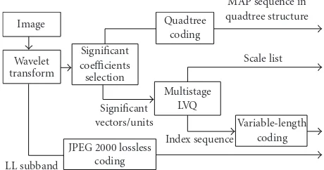
Figure 2illustrates the encoder part of the new multiscale-based multistage LVQ (MLVQ) using adaptive subband thresholding and index compression with Golomb codes. A wavelet transform is used to transform the image into a num-ber of levels. A vector or unit is obtained by subdividing the subband coefficients into certain block sizes. For example, a block size of 4×4 gives a 16 dimensional vector, 2×2 gives 4 dimensional vector, and 1×1 gives one dimensional vector. The significant vectors or units of all subbands are identified by comparing the vector energy to certain thresholds. The location information of the significant vectors is represented in ones and zeros, defined as a MAP sequence which is coded using quadtree coding. The significant vectors are saved and passed to the multistage LVQ (MLVQ). The MLVQ produces two outputs, that is, the scale list and index sequence, which are then run-length coded. The lowest frequency subband is coded using the JPEG 2000 lossless coding. The details of

Image Quadtree

coding

MAP sequence in quadtree structure

Wavelet transform

Significant coefficients selection

Multistage LVQ

Scale list

Significant

vectors/units Variable-length coding Index sequence

LL subband

JPEG 2000 lossless coding

Figure2: MLVQ encoder scheme.

MLVQ and the generation ofM-stage codebook for a par-ticular subband are described inSection 4.3.

4.2. Adaptive subband thresholding

The threshold setting is an important entity in searching for the significant coefficients (vectors/units) in the subband. A vector or unit which consists of the subband coefficients is considered significant if its normalized energyEdefined as

E= w(k) NkxNk

Nk

i=1 Nk

j=1

Xk(i,j)2 (13)

is greater than a thresholdTdefined as

T=

av

100×threshold parameter 2

, (14)

Stage 1

Stage 2

Stage 3

Initialization

Inter-level DWT setup

Thresholds optimization

End

(a) Adaptive subband thresholding scheme

For DWT level 1 to 3

Find direction

Th ParamUp

Th ParamDown T

F Num vector<

total vector

End (b) Thresholds optimization (stage 3)

Figure3

code the remaining subbands and bitbudgetis the total bit bud-get. The following relationships are defined:

bitbudget=R×(r×c)=LL sb bits + other sb bits,

total no vectors

=

Lmax

i=1

(other sb bits−0.2×other sb bits−3×8)

ρ

whereρ= ⎧ ⎨ ⎩

6, n=4, 3, n=1. (15)

In this work the wavelet transform level (Lmax) is 3, and we are approximating 20% of the high-frequency subband bits to be used to code the MAP data. ForZnlattice quantizer with codebook radius (m=3), the denominatorρis 6 (6-bit index) forn=4 or 3 (3-bit index) forn=1. The last term in (15) accounts for the LVQ scale factors, where there are 3 high-frequency subbands available at every wavelet trans-form level, and each of the scale factors is represented by 8 bits.

The adaptive threshold algorithm can be categorized into three stages as shown by the flow diagram inFigure 3(a). The first stage (initialization) calculates the initial threshold using (14), and this value is used to search the significant coeffi -cients in the subbands. Then the sifted subbands are used to reconstruct the image and the initial distortion is calculated. In the second stage (inter-level DWT setup) the algorithm optimizes the threshold between the wavelet transform lev-els. Thus in the case of a 3-level system there will be three threshold values for the three different wavelet levels.

An iterative process is carried out to search for the op-timal threshold setup between the wavelet transform levels. The following empirical relationship between threshold val-ues at different levels is used:

Tl= ⎧ ⎪ ⎨ ⎪ ⎩

Tinitial, forl=1,

Tinitial

(l−1)×δ, forl >1,

(16)

where Tinitial is the initial threshold value, Tl indicates the threshold value at DWT level l, and δ is an incremental counter.

In the search process every time the value ofδis incre-mented the above steps are repeated for calculating the dis-tortion and resulting output number of vectors that are used. The process will stop and the optimized threshold values are saved once the current distortion is higher than the previous one.

The third stage (thresholds optimization) optimizes the threshold values for each subband at every wavelet transform level. Thus there will be nine different optimized threshold values. The three threshold values found in stage 2 above are used in subsequent steps for the “threshold parameter” ex-pression derived from (14) as follows:

threshold parameter=

100 av

Tl wherel=1, 2, 3. (17)

In this stage the algorithm optimizes the threshold by in-creasing or lowering the “threshold parameter.” The detail flow diagram of the threshold optimization process is shown inFigure 3(b).

The first process (find direction) is to identify the direc-tion of the “threshold parameter” whether up or down. Then the (Th ParamUp) algorithm processes the subbands that have the “threshold parameter” going up. In this process, ev-ery time the “threshold parameter” value increases, a new threshold for that particular subband is computed. Then it searches the significant coefficients and the sifted subbands are used to reconstruct the image. Also the number of signif-icant vectors within the subbands and resulting distortion are computed. The optimization process will stop, and the opti-mized values are saved when the current distortion is higher than the previous one or the number of vectors has exceeded the maximum allowed.

Significant vectors LVQ-1 LVQ-2 LVQ-M α1 α2 αM QV1 QV2 QVM

α1×QE1

αM−1×QEM−1

1 . . . N 1 . . . N 1 . . . N CB-1 Index 1 0 1 1 34

13 . . . . . . 0 1 0 1

CB-2 Index 0 0 0 1 1

14 . . . . . . 0 1 0−1

CB-M Index 0 0 0−1 2

7 . . . . . . . . .

1 0 0 0 M-stage codebook and the

corresponding indexes

Figure4: MLVQ process of a particular subband.

as the lower bound. The optimized values are saved after the current distortion is higher than the previous one or the number of vectors has exceeded the maximum allowed.

4.3. Multistage lattice VQ

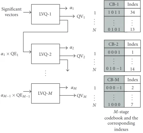
The multistage LVQ (MLVQ) process for a particular sub-band is illustrated inFigure 4. In this paper we chose theZn lattice quantizer to quantize the significant vectors. For each LVQ process, the input vectors are first scaled and then the scaled vectors are quantized using the quantizing algorithm presented inSection 3.3. The output vectors of this algorithm are checked to make sure that they are confined in the cho-sen spherical codebook radius. The output vectors that ex-ceed the codebook radius are rescaled and remapped to the nearest valid codeword to produce the final quantized vec-tors (QV). The quantization error vecvec-tors are obtained by subtracting the quantized vectors from the scaled vectors. Therefore each LVQ process produces three outputs, that is, the scale factor (α), quantized vectors (QV), and the quanti-zation error vectors (QE).

The scaling procedure for each LVQ of the input vectors uses the modification of the work presented in [3]. As a re-sult of these modifications, we can use the optimum setup (obtained from experiment) for codebook truncation where the input vectors reside in both granular and overlap regions for LVQ stage one. At the subsequent LVQ stages the input vectors are forced to reside only in granular regions. The first LVQ stage processes the significant vectors and produces a scale factor (α1), the quantized vectors (QV1) or codewords, and the quantization error vectors (QE1), and so forth. Then the quantization error vectors (QE1) are “blown out” by mul-tiplying them with the current stage scale factor (α1). They are then used as the input vectors for the subsequent LVQ

stage, and this process repeats up to stageMuntil the allo-cated bits are exhausted.

Figure 4illustrates the resultingM-stage codebook gen-eration and the corresponding indexes of a particular sub-band. At each LVQ stage, a sphericalZnquantizer with code-book radius (m = 3) is used. Hence for four dimensional vectors, there are 64 lattice points (codewords) available with 3 layers codebook [3]. The index of each codeword is rep-resented by 6 bits. If the origin is included, the outer lattice point will be removed to accommodate the origin. In one di-mensional vector there are 7 codewords with 3 bits index rep-resentation. If a single stage LVQ producesNcodewords and there areMstages, then the resulting codebook size isM×N

as shown inFigure 4. The indexes ofM-stage codebook are variable-length coded using the Golomb codes.

The MLVQ pseudo code to process all the high-frequency subbands is described in Figure 5. The Lmax indicates the number of DWT level. In this algorithm, the quantization errors are produced for an extra set of input vectors to be quantized. The advantage of “blowing out” the quantization error vectors is that they can be mapped to many more lattice points during the subsequent LVQ stages. Thus the MLVQ can capture more quantization errors and produce better im-age quality.

4.4. Lattice codebook index compression

Run-length coding is useful in compressing binary data se-quence with long runs of zeros. In this technique each run of zeros is represented by integer values or symbols. For ex-ample, a 24-bit binary sequence {00000000001000000001}

can be encoded as an integer sequence{10, 8}. If each run-length integer is represented by 8-bit, the above sequence can be represented as 16-bit sequence. This method is inefficient when most of the integer symbols can be represented with less than 8-bits or when some of the integer symbols exceed the 8-bit value. This problem is solved using a variable-length coding with Golomb codes, where each integer symbol is rep-resented by a unique bit representation of different Golomb codes length [17].

In our work, we use variable-length coding to compress the index sequence. First we obtained the value ofbas follows assuming thatXis a binary sequence with lengthN:

P(0)=p; P(1)=1−p= N i=1xi

N

; xi∈X. (18)

From (4) we can derive the value ofb

b=round

− 1

log₂(1−δ)

; whereδ= Ni=1xi

N

.

(19)

Calculate leftover bits after baseband coding

No

Leftover bits>0

For DWT level=Lmax: 1 Yes

For subband type=1 : 3

Prompt the user for inadequate

bit allocation

Scale the significant vectors (M=1) or QE vectors, and save into a scale record Vector quantize the scaled

vectors, and save into a quantized vectors record Quantization error vectors=

(scaled vectors-quantized vectors)xsignificant vectors

scale (M=1) or input vectors scale Input vector=quantization

errors vectors Calculate leftover bits, and

incrementM Yes

No End

leftover bits>0

Figure5: Flow diagram of MLVQ algorithm.

is more concentrated on the first codebook level and origin when the multistage is greater than one. This is due to the fact that the MLVQ has been designed to force the quantized vectors to reside in the granular region if the multistage has more than 1 stage as explained inSection 4.3.Figure 6 illus-trates the index compression scheme using variable-length coding with Golomb codes for 4-dimensional vector code-book indexes.

The compression technique involves two steps for the case of stage one of the MLVQ. First the index sequence is changed to binary sequence, and then split into two parts, that is, the higher nibble and the lower nibble. The compres-sion is done only on the higher nibble since it has more ze-ros and less ones. The lower nibble is uncompressed since it has almost 50% zeros and ones.Figure 6illustrates the index compression technique for MLVQ of stage one. The higher nibble index column bits are taken, and they are jointed to-gether as a single row of bit sequence S. Then the coded sequence CS is produced via variable length coding with Golomb codes with parameterb=4. FromFigure 1(a), the

first run-length (l1 = 9) is coded as {11001}, the second run-length (l2 = 0) is coded as{000}, the third run-length (l3=1) is coded as{001}, and so forth. For the subsequence stages for 4-dimensional vector of MLVQ, the entire data will be compressed rather than dividing them into the higher and lower nibbles. For 1 dimensional vector, the codebook indexes are represented as 3-bit integers and the whole bi-nary data are compressed for every MLVQ stage. In this work, the variable length coding with Golomb codes provides high compression on the index sequences. Thus more leftover bits are available for subsequent LVQ stages to encode quantiza-tion errors and yield better output quality.

5. SIMULATION RESULTS

Index Higher nibble Lower nibble

2 0 0 0 0 1 0

3 0 0 0 0 1 1

4 0 0 0 1 0 0

9 0 0 1 0 0 1

5 0 0 0 1 0 1

1 0 0 0 0 0 0

7 0 0 0 1 1 1

15 0 0 1 1 1 1

12 0 0 1 1 0 0

52 1 1 0 1 0 0

40 1 0 1 0 0 0

12 0 0 1 1 0 0

60 1 1 1 1 1 1

S= {0 0 0 0 0 0 0 0 0 1 1 0 1 0 0. . .1 1 1} l1=9 l2=0 l3=1 b=4

CS= {1 1 0 0 1 0 0 0 0 0 1. . .}

Figure6: Index sequence compression (multistage=1).

vectors, and block size 1×1 results in one dimensional vector. In this work the block size 1×1 is used in the lower subbands with maximum codebook radius set to (m=2). In this case, every pixel can be lattice quantized to one of the following values{0,±1,±2}. Since the lower subbands contain more significant data, there are higher number data being quan-tized to either to{±2}(highest codebook radius). This in-creases the codebook index redundancy resulting in a higher overall compression via entropy coding using the variable-length coding with Golomb codes.

5.1. Incremental results

In MLVQ the quantization errors of the current stage are “blown out” by multiplying them with the current scale fac-tor. The advantage of “blowing out” the quantization errors is that there will be more lattice points in the subsequence quantization stages. Thus more residual quantization errors can be captured and enhance the decoded image quality. Fur-thermore, in this work we use the block size of 1×1 in the lower subbands. The advantage is as explained as above. The block size is set to 2×2 at levels one and two, and 1×1 for lev-els three and four.Figure 7shows the effect of “blowing out” technique and the results are compared to Man’s codec [2]. In this scheme the image is decomposed to four DWT levels, and tested on image “Lena” of size 512×512. The incremen-tal results for image compression scheme with 2×2 block size for all four levels of WT can be found in [23]. In addition, the performance of MLVQ at 0.17 bpp (>32 dB) which is better as compared to the result found in [3] for image lena with PSNR 30.3 dB.

5.2. Comparison with other VQ coders

Besides comparison with Man’s LVQ [2], we also include the comparison with other VQ works that incorporate the con-cept of EZWzerotreeprediction. Therefore, we compare the

26 28 30 32 34 36 38

PSNR

(dB)

0 0.1 0.2 0.3 0.4 0.5 Bit rate (bpp)

MLVQ Man’s LVQ

Figure7: Comparison with Man’s LVQ [2] for image Lena 512×

512.

Table1: Performance comparison at bit rate 0.2 bpp.

Grey image VLVQ-VSPHIT

(entropy coded) VSPECK MLVQ JPEG 2000

Lena 32.89 33.47 33.51 32.96

Goldhill 29.49 30.11 30.21 29.84

Barbara 26.81 27.46 27.34 27.17

MLVQ without adaptive threshold algorithm with the VLVQ of VSPHIT presented in [12]. In addition, the comparison is also made with the VSPECK image coder presented in [14].

23 25 27 29 31

PSNR

0 0.1 0.2 0.3 0.4 0.5 0.6 (bpp)

JPEG2000 MLVQ:Tconstant MLVQ:Tadaptive

Figure8: Test image “goldhill.”

23 25 27 29 31 33

PSNR

0 0.1 0.2 0.3 0.4 0.5 0.6 (bpp)

JPEG2000 MLVQ:Tconstant MLVQ:Tadaptive

Figure9: Test image “camera.”

5.3. Effect of adaptive thresholding

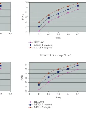
The grey (8-bit) “Goldhill,” “camera,” “Lena,” and “Clown” images of size 256×256 are used to test the effect of adap-tive subband thresholding to the MLVQ image compression scheme. The block size is set to 2×2 at level one, and 1×1 for levels two and three. The performance results of the new image coding scheme with constant and adaptive threshold are compared with JPEG 2000 [9], respectively, as shown in Figures 8,9,10,11. It is clear that using the adaptive sub-band thresholding algorithm with MLVQ gives superior per-formance to either the JPEG 2000 or the constant subband thresholding with MLVQ scheme.

Figure 12 shows the visual comparison of test image “Camera” between the new MLVQ (adaptive threshold) and JPEG 2000 at 0.2 bpp. It can be seen that the new MLVQ (adaptive threshold) reconstructed images are less blurred than the JPEG 2000 reconstructed images. Furthermore it produces 2 dB better PSNR than JPEG 2000 for the “camera” test image.

23 25 27 29 31 33 35

PSNR

0 0.1 0.2 0.3 0.4 0.5 0.6 (bpp)

JPEG2000 MLVQ:Tconstant MLVQ:Tadaptive

Figure10: Test image “lena.”

22 24 26 28 30 32 34

PSNR

0 0.1 0.2 0.3 0.4 0.5 0.6 (bpp)

JPEG2000 MLVQ:Tconstant MLVQ:Tadaptive

Figure11: Test image “clown.”

Table2: Computational complexity based on grey Lena of 256×256 (8 bit) at bit rate 0.3 bpp.

Codec 1 Codec 2

Total CPU time (s) 23.98 Total CPU time (s) 180.53 Constant threshold 0.0% Adaptive threshold 86.3%

MLVQ 100% MLVQ 13.7%

5.4. Complexity analysis

(a) Original “camera” (b) JPEG 2000, (26.3 dB) (c) MLVQ, (28.3 dB)

Figure12

6. CONCLUSIONS

The new adaptive threshold increases the performance of the image codec which itself is restricted by the bit alloca-tion constraint. The lattice VQ reduces complexity as well as computation load in codebook generation as compared to LBQ algorithm. This facilitates the use of multistage quanti-zation in the coding scheme. The multistage LVQ technique presented in this paper refines the quantized vectors, and re-duces the quantization errors. Thus the new multiscale mul-tistage LVQ (MLVQ) using adaptive subband thresholding image compression scheme outperforms JPEG 2000 as well as other recent VQ techniques throughout all range of bit rates for the tested images.

ACKNOWLEDGMENT

The authors are very grateful to the Universiti Sains Malaysia for funding the research through teaching fellowship scheme.

REFERENCES

[1] S. P. Voukelatos and J. Soraghan, “Very low bit-rate color video coding using adaptive subband vector quantization with dy-namic bit allocation,”IEEE Transactions on Circuits and Sys-tems for Video Technology, vol. 7, no. 2, pp. 424–428, 1997. [2] H. Man, F. Kossentini, and M. J. T. Smith, “A family of efficient

and channel error resilient wavelet/subband image coders,” IEEE Transactions on Circuits and Systems for Video Technol-ogy, vol. 9, no. 1, pp. 95–108, 1999.

[3] M. Barlaud, P. Sole, T. Gaidon, M. Antonini, and P. Mathieu, “Pyramidal lattice vector quantization for multiscale image coding,”IEEE Transactions on Image Processing, vol. 3, no. 4, pp. 367–381, 1994.

[4] T. Sikora, “Trends and perspectives in image and video cod-ing,”Proceedings of the IEEE, vol. 93, no. 1, pp. 6–17, 2005. [5] A. S. Akbari and J. Soraghan, “Adaptive joint subband vector

quantisation codec for handheld videophone applications,” Electronics Letters, vol. 39, no. 14, pp. 1044–1046, 2003. [6] D. G. Jeong and J. D. Gibson, “Lattice vector quantization for

image coding,” inProceedings of IEEE International Conference on Acoustics, Speech and Signal Processing (ICASSP ’89), vol. 3, pp. 1743–1746, Glasgow, UK, May 1989.

[7] J. H. Conway and N. J. A. Sloane,Sphere-Packings, Lattices, and Groups, Springer, New York, NY, USA, 1988.

[8] F. F. Kossentini, M. J. T. Smith, and C. F. Barnes, “Necessary conditions for the optimality of variable-rate residual vector quantizers,”IEEE Transactions on Information Theory, vol. 41, no. 6, part 2, pp. 1903–1914, 1995.

[9] A. N. Skodras, C. A. Christopoulos, and T. Ebrahimi, “The JPEG 2000 still image compression standard,”IEEE Signal Pro-cessing Magazine, vol. 18, no. 5, pp. 36–58, 2001.

[10] J. M. Shapiro, “Embedded image coding using zerotrees of wavelet coefficients,”IEEE Transactions on Signal Processing, vol. 41, no. 12, pp. 3445–3462, 1993.

[11] A. Said and W. A. Pearlman, “A new, fast, and efficient im-age codec based on set partitioning in hierarchical trees,” IEEE Transactions on Circuits and Systems for Video Technol-ogy, vol. 6, no. 3, pp. 243–250, 1996.

[12] D. Mukherjee and S. K. Mitra, “Successive refinement lattice vector quantization,”IEEE Transactions on Image Processing, vol. 11, no. 12, pp. 1337–1348, 2002.

[13] W. A. Pearlman, A. Islam, N. Nagaraj, and A. Said, “Efficient, low-complexity image coding with a set-partitioning embed-ded block coder,”IEEE Transactions on Circuits and Systems for Video Technology, vol. 14, no. 11, pp. 1219–1235, 2004. [14] C. C. Chao and R. M. Gray, “Image compression with a vector

speck algorithm,” inProceedings of IEEE International Confer-ence on Acoustics, Speech and Signal Processing (ICASSP ’06), vol. 2, pp. 445–448, Toulouse, France, May 2006.

[15] A. O. Zaid, C. Olivier, and F. Marmoiton, “Wavelet im-age coding with adaptive dead-zone selection: application to JPEG2000,” inProceedings of IEEE International Conference on Image Processing (ICIP ’02), vol. 3, pp. 253–256, Rochester, NY, USA, June 2002.

[16] A. Chandra and K. Chakrabarty, “System-on-a-chip test-data compression and decompression architectures based on Golomb codes,”IEEE Transactions on Computer-Aided Design of Integrated Circuits and Systems, vol. 20, no. 3, pp. 355–368, 2001.

[17] S. W. Golomb, “Run-length encodings,”IEEE Transactions on Information Theory, vol. 12, no. 3, pp. 399–401, 1966. [18] J. Senecal, M. Duchaineau, and K. I. Joy, “Length-limited

[19] A. A. Gersho and R. M. Gray,Vector Quantization and Signal Compression, Kluwer Academic, New York, NY, USA, 1992. [20] J. D. Gibson and K. Sayood, “Lattice quantization,” in

Ad-vances in Electronics and Electron Physics, P. Hawkes, Ed., vol. 72, chapter 3, Academic Press, San Diego, Calif, USA, 1988.

[21] N. J. A. Sloane, “Tables of sphere packings and spherical codes,”IEEE Transactions on Information Theory, vol. 27, no. 3, pp. 327–338, 1981.

[22] J. H. Conway and N. J. A. Sloane, “Fast quantizing and decod-ing algorithms for lattice quantizers and codes,”IEEE Transac-tions on Information Theory, vol. 28, no. 2, pp. 227–232, 1982. [23] M. F. M. Salleh and J. Soraghan, “A new multistage lattice VQ (MLVQ) technique for image compression,” inEuropean Signal Processing Conference (EUSIPCO ’05), Antalya, Turkey, September 2005.

M. F. M. Sallehwas born in Bagan Serai, Perak, Malaysia, in 1971. He received his B.S. degree in electrical engineering from Polytechnic University, Brooklyn, New York, US, in 1995. He was then a Software Engineer at Motorola Penang, Malaysia, in R&D Department until July 2001. He obtained his M.S. degree in communication engineering from UMIST, Manchester, UK, in 2002. He has completed his Ph.D. degree

in image and video coding for mobile applications in June 2006 from the Institute for Communications and Signal Processing (ICSP), University of Strathclyde, Glasgow, UK.

J. Soraghanreceived the B.Eng. (first class honors) and the M.Eng.S. degrees in 1978 and 1982, respectively, both from University College Dublin, Dublin, Ireland, and the Ph.D. degree in electronic engineering from the University of Southampton, Southamp-ton, UK, in 1989. From 1979 to 1980, he was with Westinghouse Electric Corpora-tion, USA. In 1986, he joined the Depart-ment of Electronic and Electrical