Modelling and control of the flame temperature distribution using probability density function shaping

Modelling and control of the flame

temperature distribution using

probability density function shaping

Xubin Sun

1

, Hong Yue

2

and Hong Wang

2

1_{Institute of Automation, Chinese Academy of Sciences, Beijing 100080, P.R. China} 2

Control Systems Centre, University of Manchester, Manchester M60 1QD, U.K.

This paper presents three control algorithms for the output probability density function (PDF) control of the 2D and 3D flame distribution systems. For the 2D flame distribution systems, control methods for both static and dynamic flame systems are presented, where at first the temperature distribution of the gas jet flames along the cross-section is approximated. Then the flame energy distribution (FED) is obtained as the output to be controlled by using a B-spline expansion technique. The general static output PDF control algorithm is used in the 2D static flame system, where the dynamic system consists of a static temperature model of gas jet flames and a second-order actuator. This leads to a second-order closed-loop system, where a singular state space model is used to describe the dynamics with the weights of the B-spline functions as the state variables. Finally, a predictive control algorithm is designed for such an output PDF system. For the 3D flame distribution systems, all the temperature values of the flames are firstly mapped into one temperature plane, and the shape of the temperature distribution on this plane can then be controlled by the 3D flame control method proposed in this paper. Three cases are studied for the proposed control methods and desired simulation results have been obtained.

Key words:B-spline expansion and model predictive control; flame temperature distribution probability density function (PDF).

Address for correspondence: Xubin Sun, Institute of Automation, Chinese Academy of Sciences, Beijing 100080, P.R. China, E-mail: [email protected]

Hong Wang is also affiliated with Northeastern University as a Changjiang Professor, P.R. China

Nomenclature

r Horizontal abscissa

x Vertical ordinate

u Vertical velocity

v Horizontal velocity

T Temperature

T0 Temperature at the nozzle

T Temperature at(temperature in the environment)

Tm Temperature at the symmetric axis

g Kinematical coefficient of the viscosity of the laminar flow cp Specific heat capacity of the fuel

si Mass fraction for componenti,asi1

r /ar_i;Density of the mixture

Yi Reaction heat of the componenti

b(x) Flame boundary

Re0 The Renault number at the nozzle

u0 The fuel jet velocity at the nozzle

d0 Nozzle diameter

g(x,u0) PDF,g(x,r,u0) for the 3D flame

Bi(x) Theith basis function

C(x) Matrix made up of B-spline basis functions V(u0) Weights vector of the B-spline functions

J Performance function

g(x) The given target PDF for the 3D flame

1. Introduction

To improve the efficiency and safety of various boilers used in industries, the flame temperature distribution (FTD) must be well controlled (Fuet al., 1989). Generally, the source fuels of the boiler can be either blast furnace gas or pulverized coals. For the blast furnace gas case, the flame at each burner will be a gas turbulent jet flame when the fuel jet velocity is higher than a certain threshold value, and will be a gas flamelet jet flame when the velocity is lower (Pope, 1985). However, for the pulverized coals case, the flame at each burner will be of two-phase turbulent reactive flows. This means that the efficiency of the boiler is mostly determined by the status of each burner flame, which can be controlled by dynamic FTD control methods. In this context, the flame distribution can be regarded as a probability density function (PDF), where the recently developed PDF shape control can be applied (Wang, 2000). For the gas jet flame, a static model (Fuet al., 1989) has been established and used in the 2D closed-loop control systems.

realized a closed-loop control system of the boiler flame by the radiant energy obtained from the temperature of the flame. Serial control was employed to solve the large inertia problem through the radiant energy as an intermediate variable. Wang

et al. (1995) introduced the concept of energy balance to realize the flame distribution

control. More recently, a static closed-loop control system has been investigated in Sun and Wang (2004), where a static 2D flame temperature distribution model (Fu et al., 1989) was firstly established. Flame energy distribution (FED) was then obtained from the static flame model as the output PDF. An algorithm using the PDF control concept was designed to realize the required PDF shaping. Moreover, a predictive control algorithm for the dynamic flame distribution system was presented (Sun and Wang, 2005), where the FED was also seen as the output PDF density function. However, different from the work in Sun and Wang (2004) a second-order actuator was introduced to simulate the dynamic characteristics in the real flame systems. The FED is then approximated by the B-splines functions (Wang, 2000; Yue and Wang, 2003) whose weights are taken as state variables of the dynamic system. To represent such a dynamic system, a singular state space model (Dai, 1989) was designed for the output PDF system. Stability was analysed for such a closed-loop system with predictive PDF control. It has been shown that the boundness of the first two state variables can guarantee the stability of the closed-loop system because a singular state space model is used in this system.

The 2D flame control methods are mainly designed for an axially symmetrical 3D flame distribution system, which can be easily simplified into a 2D flame distribution model. For a normal 3D flame distribution system, the 3D flame control method can be formulated where all the temperature values in the boiler are mapped into one cross-section. In practice, the temperature image captured at the top of boiler can be seen as the mapped temperature cross-section, which can well reflect the status of the boiler. A 3D flame control method is presented in this paper, the aim is to make the temperature distribution as close as possible to the given temperature distribution. Bivariate B-splines are used in the 3D flame modelling, and the output PDF control method is presented for such a 3D model, which is followed by a case study.

2. 2D flame model representation

2.1 Flame model simplification

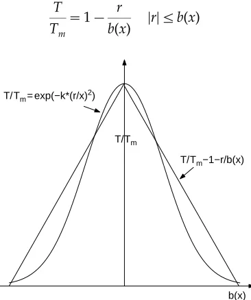
In practice, the gas flamelet jet flame distribution is of a 3D nature, which is axially symmetrical (Fu et al., 1989). Therefore, a 2D temperature distribution model can be adopted to describe the 3D flame distribution as shown in Figure 1, where d0 is

the diameter of the fuel injection nozzle, u0 is the speed of the fuel injection at the

nozzle, x is the vertical ordinate, r is the horizontal abscissa, and b(x) is the flame boundary. The two arcs are the isotherms of the jet flame.

T Tm

exp

K

_r

x

2

(1)

where T is the temperature at the point (x,r), Tm is the temperature at the

corresponding point on the axis (x, 0) and K is a coefficient with a value between 82.0 and 92.0, which is obtained from an experimental setup. To simplify the model, the following double biases distribution is used to approximate the above Gaussian distribution

T Tm

1 r

b(x) ½r½5b(x) (2)

T/T_m

b(x) T/T_m−1−r/b(x) T/T_m= exp(−k*(r/x)2₎

Figure 2 Temperature distribution in a cross-section before and

after approximation

d0

u₀

x

r b(x)

A satisfactory solution can be obtained from the conservation equations after such an approximation.

2.2 Flame model solution

It is assumed that the flame is the uncompressible steady flow and columned free jet flame. Based upon some specific boundary and initial conditions, the FTD model can be obtained by solving the continuity, momentum, energy and mass balance conservations, leading to the following flame temperature model

T(x;r)T

(T0T) s_FY_F

cp

t(x;r)sFYF

cp

(3)

where the subscript F ins_F andQF stand for the fuel flows. For the flamelet flows,

t(x,r) in (3) is given by

t(x;r)

1 8

Re0

x d0

1

1

ffiffiffi 2 3 s

r d0

1 8

Re0

x d0

1

(4)

where Re0is the Renault number at the nozzle and it is defined by

Re0

u0d0

g (5)

In (4), the input u0 controls the value oft(x,r). Furthermore,u0directly controls the

temperature value of T(x,r) in (3). In our case study, the parameters in the flame model have been selected as follows:

FuelCO

cp2078:6 J=kgK)

YF282:84 kJ=mol

d00:01 m

g3:695105

T0500 K

8 > > > > > > < > > > > > > :

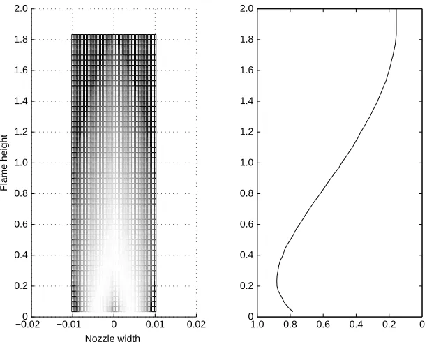
The desired FTD can be obtained though (3) and (4) with the parameters given above. The FED can then be calculated from the FTD. Physically, the flame energy is defined as the sum of all the temperature values in each horizontal cross-section, then the FED can be calculated from

g(x;u0(k))

g

g

g

(6)

corresponding FEDg(x,u0(k)) is shown on the right-hand side of Figure 3. In this case,

the input is the fuel jet velocity u0(k)/[a,b] where k stands for the current sample time. As an FTD can be ‘one-to-one’ mapped into an FED, it is reasonable to control the flame distribution through the control of FEDs.

2.3 FED modelling

As described by Sun and Wang (2004), the FED can be approximated by the following B-splines function model

g(x;u0(k))C(x)V(u0(k))L(x) (7)

C(x)

B1(x)

Bn1(x)

g

g

B2(x)

Bn1(x)

g

g

Bn(x)

Bn1(x)

g

g

2 6 6 6 6 6 6 6 6 6 6 6 6 6 6 4

3 7 7 7 7 7 7 7 7 7 7 7 7 7 7 5

Rn1 (8)

−0.020 −0.01 0 0.01 0.02

0.2 0.4 0.6 0.8 1.0 1.2 1.4 1.6 1.8 2.0

0 0.2 0.4 0.6 0.8 1.0 1.2 1.4 1.6 1.8 2.0

0 0.2 0.4 0.6 0.8 1.0

Flame height

Nozzle width

where x/[a,b] and B_i(x)(i/1, 2, . . .,n/1) are a set of pre-specified B-spline basis functions and

V(u0(k))[v1(uk);v2(uk);. . .;vn(uk)] T

Rn1

(9)

L(x)

g

Bn1(x)dx

1

Bn1(x)R11 (10)

wherevi(uk)(i/1, 2, . . .,n) are the weights of the B-spline basis functions. This means that the control of the flames distribution can be realized by controlling these weights in the B-spline model.

3. 2D static system modelling and control

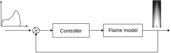
The process to be controlled is the static jetting flame model as shown in (3)(4), where the output is the FTD, which is a 2D distribution along (x,r) directions (Figure 1). However, since the flame is symmetrical, another distribution, namely the FED, can be used as a feedback for the closed-loop control. In this case, the input

u0(k)/[0, 2] is the fuel jet velocity. As the FTD can be retrieved fromg(x,u₀(k)) using the symmetrical nature of the flames, the aim of the controller design is to make g(x,u0(k)) as close as possible to a given FED. Asg(x,u0(k)) is the ratio of the energy in

each cross-section to the total energy as shown in (6), it can also be regarded as a PDF, where the recently developed stochastic distribution theory (Wang, 2000) can be directly applied to control the shape of g(x,u0(k)). A closed-loop flame distribution

control system can be established as shown in Figure 4. For this static system, the FED can be modelled using the B-splines approximation method as (7). The performance function is selected as follows

J(u0(k))

g

0

(g(x;u0(k))g(x)) 2

dx (11)

where g(x) is the given target FED function. It can be seen that such a performance function measures the difference between the actual and the target FED distributions. Minimizing u0 with respect to this performance function would therefore obtain the

required control action that can make g(x,u0(k)) as close as possible to g(x). By

substituting (7) into (11), and denoting

Controller Flame model

X

g

0

CT(x)C(x)dxR(nn)

h

g

0

(g(x)L(x))C(x)dxR1n

g₀

g

0

(g(x)L(x))2dx

the control input can be calculated from the recursive form

u0(k)u0(k1)2m(V

T

(u)Sh)@V(u)

@u ½uu0(k1) (12)

where m/0 is a pre-specified step length. This 2D static FED control can be easily realized in practice. However, it ignores the dynamics of the whole flame system that includes the actuator and sensor dynamics, etc. As such, a more practical control method needs to be developed.

4. Predictive control of 2D dynamic flame

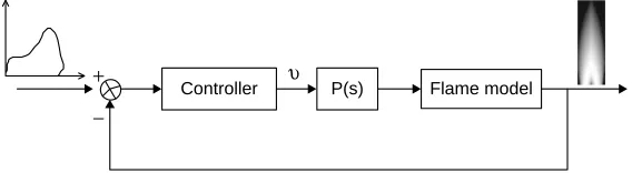
4.1 Control system structure

To consider the system dynamics, a dynamic close-loop control method is designed as shown in Figure 5. Different from the previous work in Sun and Wang (2004), a second-order actuator with a transfer functionP(s) is included in the system. As the flame dynamics are generally very fast, the dynamic model can reflect the actual situation in the flames control to a certain degree.

4.2 Predictive control algorithm

The normal state space PDF model used in Wang (2000) and Wang et al. (2005) takes the weights of the B-spline functions as its state variables and thus leads to anth-order system with the same dimension as that ofV(k). However, the real system in Figure 5 is of second order only. To simplify the model, a singular state space model is introduced as follows:

Controller Flame model

+ −

υ

P(s)

EV(k1)AV(k)Bu0(k)

g(x;u0(k))C(x)V(k)L(x)f(x;k)L(x) (13)

where det(E)/0,det(A)"/0,x/[a,b],E/Rnn, A/Rnn, B/Rn1, matricesE and

A can be selected to guarantee that only two weights in vector V(k) are dynamically related to the control input, whilst the others are the linear combination of the selected two dynamical weights. Then (13) can be generally given as:

1 1 0 ::_: 0 2 6 6 6 6 4 3 7 7 7 7 5

v1(k1)

v2(k1)

n n

vn(k1)

2 6 6 6 6 4 3 7 7 7 7 5

a1 d1 0 0 0

a2 d2 0 0 0

a3 d3 1 0 0

n n ₀ ::_{: 0}

an dn 0 0 1

2 6 6 6 6 4 3 7 7 7 7 5

v1(k)

v2(k)

n n

vn(k)

2 6 6 6 6 4 3 7 7 7 7 5 b1 b2 n n bn 2 6 6 6 6 4 3 7 7 7 7

5u0(k) (14)

which can be further expressed as follows:

v1(k1)a1v1(k)d1v2(k)b1u0(k)

v2(k1)a2v1(k)d2v2(k)b2u0(k)

v3(k)a3v1(k)d3v2(k)b3u0(k)

n

vn(k)anv1(k)dnv2(k)bnu0(k)

8 > > > > < > > > > : (15)

The first two equations in (15) can be extracted to give

v1(k1)

v2(k1)

a1 d1

a2 d2

v1(k)

v2(k)

b1

b2

u0(k) (16)

By taking the z-transforms of (16), it can be obtained that

v1(k1)

v2(k1)

z1 a1 d1

a2 d2

v1(k1)

v2(k1)

b1

b2

u0(k) (17)

and hence

v1(k1)

v2(k1)

Iz1 a1 d1

a2 d2

1

b1

b2

u₀(k) (18)

Substituting (18) into (15), the following decoupled system can be formulated:

v1(k1)e11v1(k)e12v1(k1)e16u0(k)e17u0(k1)

v2(k1)e21v1(k)e22v1(k1)e26u0(k)e27u0(k1)

v3(k)e31v1(k1)e32v1(k2)e33v2(k1)e34v2(k2) e35u0(k)e36u0(k1)e37u0(k2)

v4(k)e41v1(k1)e42v1(k2)e43v2(k1)e44v2(k2) e45u0(k)e46u0(k1)e47u(k2)

n

vn(k)en1v1(k1)en2v1(k2)en3v2(k1)en4v2(k2) en5u0(k)en6u0(k1)en7u0(k2)

8 > > > > > > > > < > > > > > > > > :

(20)

In the above equations, all the weights are represented by v1, v2andu0.

The performance function based ong(x,k) is used to identify the model parameters as in Wang (2000) and Wang et al. (2005). Its purpose is to make the current output g(x,k) and the modelled output PDFgg(x,k) as close as possible. Such a performance

function is formulated as follows

J(g(x;k))

g

b a

(g(x;k)g_g(x;k))2dx

However, it is computationally difficult to estimate a large number of parameters of the singular model using any identification methods. As such, the system identification based on vi(k) is used in this paper and its purpose is to make each

vi(k) andv g

i;that is theith weight of the B-spline approximation, as close as possible.

Such a performance function is represented as

J(vi(k))(vi(k)v g i(k))

2

(i1;2;. . .;n)

Theorem 1. When the B-spline functions are of second order, system identification

based on g(x,k) is equivalent to the one based on the weightsvi(k).

Proof. If the B-spline functions are of second order, then they have the

follow-ing feature:

g

Ci(x)Cj(x)dx

0 ½ij½1

M1"0 ½ij½0

M2"0 ½ij½1

8 < :

i1;2;. . .;n; j1;2;. . .;n

where M1andM2 are non-zero constants.

Compare the performance function J(g(x,k)) of the identification method based on g(x;k) and the performance function J(vi(k)) i/1,2,. . .,n based on v_i(k) by using the following inequality

J(g(x;k))

g

b a

(g(x;k)g_g(x;k))2dx

g

b a

(C(x)V(k)C(x)Vg(k))

2

g

b a

C2

1(v1v

g

1) 2

dx 2

g

a

C1C2(v1v

g

1)(v2v

g

2)dx

g

b a

C2

2(v2v

g

2) 2

dx 2

g

a

Cn1Cn(vn1v

g

n1)(vnvgn)dx

. . .

g

b a

C2n(vnvgn)

2

dx (21)

According to the basic inequality 2xy5/x2/y2, this equation can be rewritten by the following inequality that shows the relation between the performance function based ong(x,k) and the performance function based onvi(k).

J(g(x;k)52

g

b a

C2

1(v1v

g

1) 2

dx 3

g

b a

C2

2(v2v

g 2) 2 dx 3

g

n1(vn1v

g n1))

2

dx2

g

b a

C2

n(vnvgn)

2

dx

2M1(v1v

g

1)

2

3M1(v2v

g

2) 2

3M1(vn1v

g n1)

2

2M1(vnvgn)

2

53nM1max

i (viv g i)

2

3nM1max

i J(vi(k)) (22)

If max

i J(vi(k))00 can be guaranteed, thenJ(g(x;k))00 will be hold. Q.E.D.

Based on this theorem, the weights equations in (19) and (20) can be identified separately. Thenf(x;k1) can be described using historical information ofv1,v2and

u0as follows:

f(x;k1)C(x)V(k1)X

n

i1

Ci(x)viv1(k2)

Xn

i1;i"2

ei1Ci(x)

v1(k3)

Xn

i1;i"2

ei2Ci(x) v2(k2)

Xn

i2

ei3Ci(x)

v2(k3)

Xn

i2

ei4Ci(x)u0(k1)

Xn

i3

ei5Ci(x)

u0(k2)

Xn

i1

ei6Ci(x)u0(k3)

Xn

i1

ei7Ci(x)

CS1(x)v1(k2)C S

2(x)v1(k3)C

S

3(x)v2(k2)

CS

4(x)v2(k3)C

S

5(x)u0(k1)C

S

6(x)u0(k2)

CS

7(x)u0(k3) (23)

where CS

j(x)a n

i1eijCi(x) (j1; 2; . . .; 7):As a result, the predicted outputs at time

f(x;k)f11v1(k1)f12v1(k2)f13v2(k1)

f₁₄v2(k2)qu0(k2)h1u0(k1)g11u0(k)

f(x;k1½k)f21v1(k)f22v1(k1)f23v2(k)

f24v2(k1)h2u0(k1)g21u0(k)g22u0(k1)

f(x;k2½k)f31v1(k)f32v1(k1)f33v2(k)f34v2(k1)

h3u0(k1)g31u0(k)g32u0(k1)g33u0(k2)

n

f(x;kNp1½k)fNp;1v1(k)fNp;2v1(k1)fNp;3v2(k)fNp;4v2(k1)

hNpu0(k1)gNp;1u0(k) gNp;Npu0(kNp1) (24)

where Np is the predictive horizon. Define vectorY and matrixF as follows:

Y[f(x;k);f(x;k1½k);. . .;f(x;kNp1½k)]T

F

f11 f12 f13 f14

f21 f22 f23 f24

n n n n

fNp;1 fNp;2 fNp;3 fNp;4

2 6 6 4

3 7 7 5

Based upon the predictive model (23), the parameters in matrix F can be obtained recursively. The first row in matrix Fis given as follows:

[f11 f12 f13 f14][0 C S

1 0 C

S 3]

and theith row in matrixF can be expressed as

[fi1 fi2 fi3 fi4][CS1 C S

2 C

S

3 C

S

4]

e11 e12 0 0

1 0 0 0

0 0 e23 e24

0 0 1 0

2 6 6 4

3 7 7 5

i2

(25i5Np)

Define vector Q which includes the information of the past timek/2 by

Q

qu0(k2)CS2v1(k2)CS4v2(k2)

0 n 0 2

6 6 4

3 7 7 5

CS

7u0(k2)C

S

2v1(k2)C

S

4v2(k2)

0 n 0 2

6 6 4

3 7 7 5

G

g₁₁

g₂₁ g₂₂

n n ::_:

g_Np;1 g_Np;2 g_Np;Np

2 6 6 4 3 7 7 5 g₁₁

g₂₁ g₁₁

n n ::_:

g_Np;1 g_Np1;1 g₁₁

2 6 6 4 3 7 7 5

Obviously G is a lower triangle matrix, where/g_i;jg_i1;j1(i]j1): Moreover, the first column of matrix Gis given by

CS 5

CS 6

CS

7f21e16f23e26

f21e17f31e16f23e27f33e26

n

[fNp2;1e17fNp1;1e16 fNp2;3e27fNp1;3e26]

2 6 6 6 6 6 6 6 6 4 3 7 7 7 7 7 7 7 7 5

RNp1

Define Nu as the control horizon. As described in the general predictive control

method, the input is allowed to change over the next Nu steps. This means that

/Du₀(kj)0;jN_u;. . .;N_p1:As a result,Gcan be rewritten as follows:

G

u0(k)

u0(k1)

n

u0(kNu1)

n

u0(kNp1)

2 6 6 6 6 6 6 4 3 7 7 7 7 7 7 5 G 1 1 1 1 1 1 2 6 6 6 6 6 6 4 3 7 7 7 7 7 7 5

u0(k1)G

1 1 1 n n ::_: 1 1 1 n n n n

1 1 1 1

2 6 6 6 6 6 6 4 3 7 7 7 7 7 7 5

Du0(k)

Du0(k1)

n Du0(kNu1)

2 6 6 4 3 7 7 5G

1 1 1 1 n 1 2 6 6 6 6 6 6 4 3 7 7 7 7 7 7 5

u0(k1)G

Du0(k)

Du0(k1)

n Du0(kNu1)

2 6 6 4 3 7 7 5

where G has been defined as:

GG

1 1 1

n n ::_: 1 1 1

n n n n

1 1 1 1

Other vectors are defined by: H h1 h2 n hNp 2 6 6 4 3 7 7 5G

1 1 n 1 2 6 6 4 3 7 7 5 CS 6 CS 7

f21e17f23e27

f31e17f33e27

n

fNp1;1e17fNp1;3e27

2 6 6 6 6 6 6 4 3 7 7 7 7 7 7 5 G 1 1 n 1 2 6 6 4 3 7 7 5

DU[Du0(k);Du0(k1);. . .;Du0(kNu1)] T

W[v1(k) v1(k1) v2(k) v2(k1)]

T

Yr(x;k)[fr(x;k) fr(x;k1) . . . fr(x;kNp1)]T

wherefr(x;k) is the given reference output. Using these vectors and matrices, equation

(24) can be rewritten as:

YGDUFWHu0(k1)Q (25)

The performance function that is used to obtain an optimal input value is selected in a form of an integration.

J(DU)

g

b a

[(YYr) T

(YYr)lDU T_D

U]dx (26)

The optimal input can then be obtained from the following equation:

@J(DU)

@DU

g

b a

GT_[GDUFWHu

0(k1)Q]lDU

dx 0 (27)

leading to

DU

g

1

g

YrFWHu0(k1)Q

dx (28)

Equation (28) produces an input sequence. However, only the first element ofDUwill be adopted to calculate the current input and applied to the system. This gives

u0(k)u0(k1)Du0(k) (29)

To realize this algorithm, the following steps should be employed:

1) Set the current sample time ask and formulate the current output PDFgk(x); 2) Use B-spline functions to estimategk(x), then the weights vectorV(k) is obtained; 3) Identify the equations using the standard recursive least-squares algorithm separately; 4) Calculate G, F, H and Q. Then calculateDU in (28);

4.3 Stability analysis

To guarantee the stability of the closed-loop control system (13) and (29), a condition needs to be established in order to guarantee the boundness and continuity of the outputg(x,u0(k)) of the closed-loop system. ObviouslyC(x) in (13) is continuous and

uniformly bounded, so the continuity and boundness ofg(x,u0(k)) can be guaranteed

if the boundness ofV(k) can be proved when the control algorithm (29) is applied to (13). As such, the control algorithm should be transferred so as to relateu0(k) directly

toV(k). As the other weights v3(k), v4(k),. . .vn(k) are all linear combinations ofv1(k)

andv2(k), the output g(x,u0(k)) will be bounded if v1(k) andv2(k) are both bounded.

As such, only the boundness of v1(k) and v2(k) needs to be considered for such a

singular system.

For this purpose, the dynamic equation ofv1(k) andv2(k) in (16) can be represented

as follows:

V1(k1)A1V1(k)B1u0(k) (30)

where V1(k)

v1(k)

v2(k)

R21_{; A}

1

a1 d1

a2 d2

R22_{; B}

1

b1

b2

R21_{: As a result, the}

stability of the closed-loop system is determined by the stability of vector V1.

It is necessary to obtain a direct relationship between V1(k) and u0(k) firstly before

the stability condition is analysed. For this purpose, denote the first row of the following matrix

g

GT_GdxlI

1

RNuNu

as vectorpR1Nu; thenDu

0(k) can be represented as

Du0(k)p

g

b a

GT[YrFWHu0(t1)Q]dx (31)

Furthermore, vector Q is divided into the following two parts:

QQuu0(k2)QvV1(k2)

q

0 n 0 2 6 6 4

3 7 7

5u0(k2)

CS

2 C

S 4

0 0

n n

0 0

2 6 6 4

3 7 7

5V1(k2)

At the same time, matrix F is represent as

FWF1V1(k)F2V1(k1)

f11 f13

f21 f23

n n

fNp;1 fNp;3

2 6 6 4

3 7 7 5 v_v1₂(₍k_k)₎

f12 f14

f22 f24

n n

fNp;2 fNp;4

2 6 6 4

3 7 7

5 v_v1₂(₍k_k1)1)

where matrix F1, which is composed of the first and third columns of matrix F,

and the fourth columns of matrix F, groups the information up to time k/1. With matrices Qu, Qv, F1 and F2, the relationship between u0 and V1 can be obtained by

rewriting Equation (29) as follows:

u0(k)u0(k1)Du0(k)

u0(k1)p

g

b a

GT_[Y

rFWHu0(t1)Q]dx

u0(k1)p

g

b a

GT[YrF1V1(k)F2V1(k1)

Hu0(t1)Quu0(k2)QvV1(k2)]dx (32)

The equation can be further written as

u0(k)

1p

g

b a

GTHdx

u0(k1)

g

b a

GTQudxu0(k2)

p

g

b a

GT[YrF1V1(k)F2V1(k1)QvV1(k2)]dx (33)

where the left-hand side of this equation consists of the information on u0 and the

right-hand side consists of the information on V1. Taking the/z transforms of this equation, it can be obtained that

u0(k)

1p

g

b a

GT_Hdx

u0(k)z1

g

b a

GT_Q

udxu0(k)z2

p

g

b a

GT[YrF1V1(k)F2V1(k1)QvV1(k2)]dx (34)

which leads to the following format

[1V₁z1_V

2z2]u0(k)p

g

b a

GT_[Y

rF1V1(k)F2V1(k1)QvV1(k2)]dx (35)

This means thatu0(k) can be represented by the current and past information ofV1to

give

u0(k)V 1

p

g

b a

GT[YrF1V1(k)F2V1(k1)QvV1(k2)]dx (36)

where V1V₁z1_V

2z2: Substituting this equation into (30), it can be obtained

that

V1(k1)A1V1(k)B1V 1

p

g

a

GT

[YrF1V1(k)F2V1(k1)QvV1(k2)]dx (37)

(1V₁z1V₂z2)V1(k1)(1V1z 1_V

2z 2

)A1V1(k)

B1p

g

b a

GT_[Y

rF1V1(k)F2V1(k1)QvV1(k2)]dx (38)

which can be rewritten as

V1(k1)

V1IA1B1p

g

b a

GT_F

1dx

V1(k)

V₂IV₁A1B1p

g

b a

GTF2dx

V1(k1)

V2A1B1p

g

b a

GT_Q vdx

V1(k2)

B1p

g

b a

GTYrdx (39)

whereIR22_{is a unit matrix. In the above equation the value of V}

1(k1) is a linear

combination ofV1(k);/V₁(k1) andV₁(k2):Simplifying this equation leads to

V1(k1)F1V1(k)F2V1(k1)F3V1(k2)F4 (40)

where

F₁V₁IA1B1p

g

b a

GT_F

1dx R22

F₂

V₂IV₁A1B1p

g

b a

GTF2dx

R22

F₃V₂A1B1p

g

b a

GT_Q

vdxR22

F₄B1p

g

b a

GTYrdx

Based upon the recursive form of V1, the value of v1(k/1) can be represented as follows

V1(k1)[F1 F2 F3]

F₁ F₂ F₃

I 0 0

0 I 0

2 4

3 5

k3

V1(3)

V1(2)

V1(1)

2 4

3

5F₄Sq(k4) (41)

where Sq(k4)[1s(0)s(1) s(k4)] is a progression term whose

s(i)[F1 F2 F3]

F₁ F₂ F₃

I 0 0

0 I 0

2 4

3 5

i

1 0 0 2 4

3

5 (i]0) (42)

Obviously, if the matrix

F₁ F₂ F₃

I 0 0

0 I 0

2 4

3

5_{is stable (ie, all its eigenvalues are inside the}

unit circle), the first term on the right-hand side of (53) will be bounded. Ifk0;then

[F1 F2 F3]

F₁ F₂ F₃

I 0 0

0 I 0

2 4

3 5

k3

0

Also, if the matrix

F₁ F₂ F₃

I 0 0

0 I 0

2 4

3

5 _{is stable, then the dynamic evolution will be}

convergent. This means that Sq(k4)B where k can be any big integer. To

summarize, we have the following theorem.

Theorem 2. Suppose that Yr and C(x) are continuous and uniformly bounded, then

the closed-loop system (13) and (29) is stable if the eigenvalues of the matrix/ F₁ F₂ F₃

I 0 0

0 I 0

2 4

3

5are all inside the unit circle.

As the dynamic termP(s) is added in the control system, the flame model becomes more complex and is also closer to practical cases than that of the static model. These two control methods can be used for the flame distribution systems that can be simplified into a 2D flame distribution. For the irregular flame distributions, 3D control methods need to be designed.

5. 3D control method

The above two flame control methods are only effective for regular flame cases, especially for axially symmetric flame distributions. To control complicated flame distributions, a 3D flame distribution control will be described in this section. Although irregular 3D flames cannot be simplified into 2D flames, it can be simplified in other ways to realize the flame shape control. Two ways can be considered, one is to select a characteristic temperature plane from the 3D temperature space as the output of the system, the other is to map all the temperature values into a given plane. After an appropriate normalization, the temperature distributiong(x,r,u0(k)) can be obtained which satisfies

g

For static irregular flames,g(x,r,u0(k)) can be modelled by B-spline functions. The aim of

the flame control is to make theg(x,r,u0(k)) as close as possible to the following given

temperature distribution.

g(x;r;uk)f(x;r;uk)L(x;r)C(x;r)V(u(k))L(x;r) (43)

where

/ CT(x;r)

B1(x;r)

Bn(x;r)

f_Bn(x;r)dxdrfB1(x;r)dxdr

B2(x;r)

Bn(x;r)

f_Bn(x;r)dxdrfB2(x;r)dxdr

n

Bn1(x;r)

Bn(x;r)

f_Bn(x;r)dxdrfBn1(x;r)dxdr

2 6 6 6 6 6 6 6 6 6 4

3 7 7 7 7 7 7 7 7 7 5

L(x;r)(f_Bn(x;r)dxdr)1Bn(x;r)

andBi(x;r)(i1; 2; . . .; n) are a series of bivariate B-spline basis functions, which can be

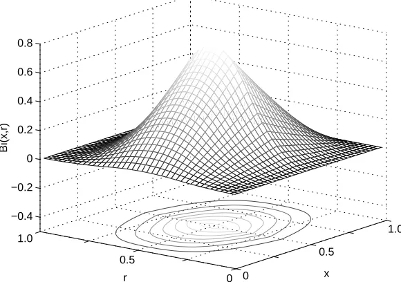
formed by taking a tensor product of two univariate B-splines as follows (Figure 6).

Bk;i(x;r)

Y2

j1

Bkjij(x) Bkxix(x)Bkrir(x)

In the above equation,krepresents the order of each B-spline, andi stands for theith B-spline.

0

0.5

1.0

0 0.5

1.0 −0.4 −0.2 0 0.2 0.4 0.6 0.8

x r

Bi(x,r)

Figure 6 Tensor product of one order 2 and one order 3 univariate

5.1 System identification

The discrete-time form of the system in (43) is presented when the system identification algorithm is considered. In (43), the term/L(x;r) is known when the B-spline functions are given. This means that only the identification of/f(x;r;u_k) should be considered.

Taking/f_k(i;j);[C₁(i;j);C₂(i;j);. . .;C_n(i;j)] i1;2;. . .;n_x;j1;2;. . .;n_rin the discrete-time with integersnxandnr;these 2D matrices can be transferred into 1D ones to read

fk[i(nx1)j]fk(i;j)

C1;2;...;n1[i(nx1)j]C1;2;...;n1(i;j)

As such, Equation (43) can be rewritten as

fkCVk (44)

where /f_kand V_k are vectors and C is a matrix. The standard least-square (LS) identification algorithm can then be used to produce

Vk(CTC)

1

CT_f

k (45)

Other identification methods can also be used in this part.

5.2 3D static flame control algorithm

The performance function is again selected as

J

gg

dxdr (46)

where g(x,r) is a given temperature distribution. Substituting (43) into (46) yields

J

gg

dxdr (47)

which can be further expressed as

JVT(u0(k))

X

V(u0(k))2hV(u0(k))g0 (48)

where it has been denoted that X

gg

h

gg

g₀

gg

@J

@u0(k)

0 (49)

Substituting (48) into (49), it can be obtained that

(VT_(u

0(k))

X

h)@V(u0(k))

u0(k)

0 (50)

Since the relationship betweenVandu0is nonlinear, the gradient method can be used

to calculate the optimal solution to give

u0(k)

i1

u0(k)

i

2m(VT(u0(k))

X

h)@V(u0)

u0

j

u0u0(k)

i

(51)

where m is a given step length, and i/1, 2, . . . .

6. Simulations and results

6.1 2D static flame control simulation

Forty second-order basis functions are used to approximate the FED curve. Since one input generates one unique FED curve, the target FED curve is determined by a given inputug. Two set of simulation results are presented where the value of the

step lengthm in Equation (12) is determined in two different ways. In the first case,m is set as a given constant value 0.2. In the second case,m is determined by the Linear Search Method of the well known LevenbergMarquardt Nonlinear Programming in the range of /(0;0:3]: In practice the range of m can be obtained based upon the response speed of the system. Indeed, the value of m determines the speed of convergence with a large m producing a fast convergence. Figure 7 shows the responses of the control input as calculated from (12). Figure 8 gives the responses of the performance function in (11). The 3D plots in Figures 9 and 10 show how the closed-loop control can be realized so as to control the distribution of FED towards its target distribution.

In the simulation, a static model of the flame distribution system was derived and used for the closed-loop control design. Under the assumption that the flame is symmetric with respect to the vertical axis, the FED function is used to realize the control of the FTD. Since such a distribution can now be measured through a video camera and an image processing, the proposed control can be used to construct an effective closed-loop control for practical flame distribution systems.

6.2 2D dynamic flame control simulation

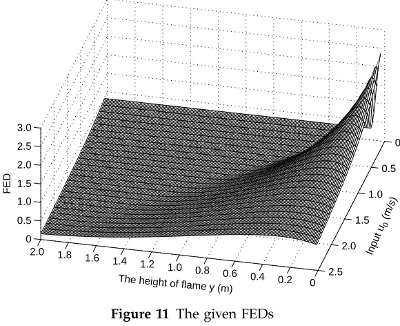
In the simulation,u0is defined in [0, 2.5] and Figure 11 (which is similar to Figure 9)

shows FEDs defined on the input interval. In this case, the target FED is given by g(x;ur

Yr(x)[fr(x;1:9348) . . . fr(x;1:9348)]

the control objective is to find a control rule so that the output FED follows the given FED as close as possible. A second-order B-spline with 41 basis functions is used to model the process withu0(1)1;l2;/N_p4;and/N_u1;2;3:The value of parameter

0 20 40 60 80 100 120 140 160 180

0 0.05 0.10 0.15 0.20 0.25 0.35

Step length = 0.2 Step length unfixed

Evaluation function J(k)

Sample time k

Figure 8 The responses of the evaluation functions

0 20 40 60 80 100 120 140 160 180

0.2 0.4 0.6 0.8 1.0 1.2 1.4 1.6 1.8 2.0

Step length = 0.2 Step length unfixed

Input u

0

Sample time k

l influences the speed of the convergence and the quantity of control. In general, a large value ofl will lead to a fast speed of the convergence. The transfer function in Figure 5 is given by

0 _0.5

1.0 _1.5

2.0 ₀

0.5 _1.0

1.5 _2.0 0 0

1 2

0 1

2

0 0.5 1.0 1.5 2.0 2.5 3.0

x

u₀

Figure 10 The estimated FED using the B-spline model

0 0.5 1.0 1.5 2.0 0 0.5 1.0 1.5 2.0 0

0 0.4 0.8 1.2 1.6 2.00 0.5 1.0 1.5 2.0 2.5

x u₀

P(s) 0:8491

s2_1:6s1

leading to the control sequence shown in Figure 12. In Figure 12,Nu2 gives the best

control sequence whenNp4.

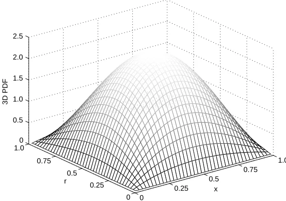
6.3 3D static flame control simulation

To test the 3D flame control algorithm, the following static flame model is used

g(x;r;u0)

xr(x1)(r1)(x1u0)(x2u0)

g

g

(52)

This PDF g(x;r;u0) can be seen as the temperature distribution of the image

captured from the top of the boiler and u0 can be regarded as the input andx,r,u

are all defined in the domain [0, 1]. In the above equation, u0 directly controls

the shape of g(x, r, u0). To simulate the system, let the initial PDF be determined

by u0/0.95, and the target PDF obtained by u₀/0.1. Define the step length as m/0.01, then six B-spline basis functions of the third-order for the x axis and four functions of the second-order for ther axis can be formed. The results are given in the Figures 1317.

0 0.2 0.4 0.6 0.8 1.0 1.2 1.4 1.6 1.8 2.0

0

0.5

1.0

1.5

2.0

2.5 0

0.5 1.0 1.5 2.0 2.5 3.0

Input u

0

(m/s)

The height of flame y (m )

FED

7. Conclusion

Three flame distribution control methods are presented for the FTD control in this paper via the use of stochastic distribution control ideas. The first two methods are

0

0.25 0.5

0.75 1.0

0 0.25 0.5 0.75 1.0

0 0.5 1.0 1.5 2.0 2.5

x r

3D PDF

Figure 13 The initial PDF of 3D static control simulation

0 10 20 30 40 50 60 70 80 90 100

1.0 1.1 1.2 1.3 1.4 1.5 1.6 1.7 1.8 1.9 2.0

Nu = 3 Nu = 1 Nu = 2 Given input

Input u

0

(k)

Sample time k

Figure 12 The 2D dynamic control sequence with differentvalues

suitable for axially symmetric flame distributions, which can be simplified into 2D flame distributions. Ignoring the system dynamics, the 2D static control can be easily realized in practice. However, the 2D dynamic control method is much closer to practical situations than the static ones because a dynamic term is added in the control system so as to represent the actuator effect in real systems. It is important to note that

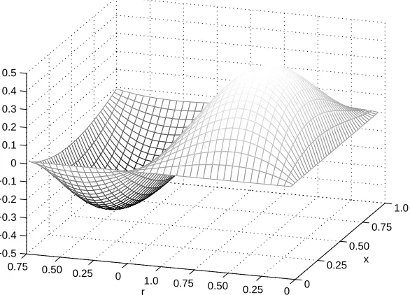
0 0.25

0.50 0.75

1.0

0 0.25 0.50 0.75 1.0 0 0.25 0.50 0.75 −0.5 −0.4 −0.3 −0.2 −0.1 0 0.1 0.2 0.3 0.4 0.5

x

r

Figure 15 The difference between the initial and given PDF

0

0.25 0.5

0.75 1.0

0 0.25 0.5 0.75 1.00 0.5 1.0 1.5 2.0 2.5 3.0

x r

3D PDF

the pre-condition for choosing the 2D control algorithms is that the flame temperature field can be presented by its FED. However, not all the FTD can satisfy such a condition. As such, a 3D flame distribution control algorithm has been proposed, which requires a high computational cost but can present more information on the dynamical evolution of the FTD. In addition, the 3D static control method is the first

0 200 400 600 800 1000 1200 1400 1600 1800 2000

0.01 0.015 0.02 0.025 0.03 0.035 0.04 0.045 0.05 0.055 0.055

J

k

Figure 17 The performance function of 3D static control

simula-tion

0 200 400 600 800 1000 1200 1400 1600 1800 2000

0.1 0.2 0.3 0.4 0.5 0.6 0.7 0.8 0.9 1

k u0

step for the dynamic controller design of 3D irregular flame distributions. The desired results have been obtained in the simulations of these methods.

The flame distribution models for static and dynamic 2D flame control are formulated based upon the assumption that all the temperature distributions on each cross-section are similar. Such a flame model cannot be controlled by the 3D algorithm. As such, a direct comparison between the 2D and 3D control algorithms is not available in this paper.

Acknowledgements

The authors would like to thank the Chinese NSF grants 60534010 and 60472065 for the support of this work.

References

Dai, L. 1989: Singular control systems. Spring-Verlag.

Fu, W.B., Zhang, Y.L. and Wang, Q.A. 1989: Combustion theory. Higher Education Press. Maciejowski, J.M.2001:Predictive control: with

constrains. Prentice Hall.

Pope, S.B. 1985: PDF methods for turbulent reactive flows.Progress in Energy and Combus-tion Science 11, 11992.

Sun, X.B.andWang, H.2004: Closed control of gas jetflames distribution using probability density function shaping techniques. In Control 2004, University of Bath, ID-088. Sun, X.B.andWang, H.2005: Stable predictive

control of gas jet flame distribution via the output probalility density function shaping. In Proceedings of the 13th Mediterrenean Con-ference on Control and Automation, Cyprus, 145863.

Tao, W.andBurkhardt, H.1994: Application of fuzzy logic and neural network to the control

of a flame process. InProceedings of the Second International Conference on Intelligent Systems Engineering, Hamburg, 23540.

Wang, H. 2000: Bounded dynamic stochastic systems: modeling and control. Spring-Verlag.

Wang, H., Zhang, J.F.andYue, H.2005: Multi-step predictive control of a PDF-shaping problem.Acta Automatica Sinica 31, 27479. Wang, J., Du, J. and Wang, S.Y. 1995: Study

and application of energy balance method and on-line thermal efficiency.Electric Power 12, 3841.

Yue, H. and Wang, H. 2003: Recent develop-ments in stochastic distribution control: a review.Measurement and Control 36, 20915. Zhou, C.H.1996: Model establishment of fuel