Comparison Of Modelling Between ARX And ARMAX Model In System Identification

(1)

COMPARISON OF MODELLING BETWEEN ARX AND ARMAX MODEL IN SYSTEM IDENTIFICATION

SITI NUR NADHIRAH BINTI NONCHIK

A report submitted

in fulfillment of the requirements for the degree of Bachelor of Mechanical Engineering

Faculty of Mechanical Engineering

UNIVERSITI TEKNIKAL MALAYSIA MELAKA

(2)

SUPERVISOR’S DECLARATION

I hereby declare that I have read this project report and in my opinion this report is sufficient in terms of scope and quality for the award of the degree of Bachelor of Mechanical Engineering.

Signature : ……….

Supervisor’s Name : ……….

(3)

DECLARATION

I declare that this project report entitled “Comparison of Modelling between ARX and ARMAX Model in System Identification” is the result of my own work except as cite in the references.

Signature : ……….

Name : ……….

(4)

DEDICATION

(5)

ABSTRACT

(6)

ABSTRAK

(7)

ACKNOWLEDGEMENTS

All praises to Allah S.W.T for helping and blessing through the entire problem that I faced during this period of final year project and to complete this final report.

Firstly, I would like to thanks my parents who are always give me their full support and encourage me to complete this project. I also want to take this opportunity to express my deepest appreciation to my supervisor, Dr. Fahmi Bin Abd Samad for his supervision, encouragement, suggestion, advice and trust throughout the duration in completion this project.

(8)

TABLE OF CONTENT PAGE DECLARATION SUPERVISOR’S DECLARATION DEDICATION ABSTRACT ABSTRAK ACKNOWLEDGEMENTS TABLE OF CONTENTS LIST OF TABLES LIST OF FIGURES

LIST OF ABBREVIATIONS LIST OF SYMBOLS

i ii iii iv v ix x xiii xiv CHAPTER

1 INTRODUCTION 1

1.1 Background 1

1.2 Problem Statement 2

1.3 Objective 2

1.4 Scope of Project 3

2 LITERATURE REVIEW 4

2.1 System Identification 4

2.1.1 Introduction 4

2.1.2 Dynamic System 4

2.1.3 Mathematical Models 7

2.1.4 System Identification Procedure 8

2.2 ARX Model 9

2.2.1 The Model Structure 9

2.2.2 Advantages and Disadvantages of ARX Model

10

(9)

2.3.1 The Model Structure 11 2.3.2 Advantages and Disadvantages of ARMAX

Model

12

2.4 Least Square Method 12

3 METHODOLOGY 14

3.1 Introduction 14

3.2 Familiarization with MATLAB Environment 16

3.3 System Identification Toolbox 16

3.3.1 Starting GUI 17

3.3.2 Import Data 18

3.3.3 Estimate Model 25

3.4 Performance Indicator 28

3.4.1 Fit 28

3.4.2 Final Prediction Error 29

3.4.3 Mean Square Error 29

4 RESULTS AND ANALYSIS 30

4.1 Introduction 30

4.2 ARX and ARMAX Model Orders and Delay 30

4.3 Model 1 31

4.3.1 Simulated Results 33

4.3.1.1 ARX 352 33

4.3.1.2 ARX 452 34

4.3.1.3 ARX 362 35

4.3.1.4 AMX 3512 36

4.3.1.5 AMX 3522 37

4.3.1.6 AMX 3532 38

4.3.2 Discussion of Fits in Model 1 39

4.3.3 Discussion of FPE in Model 1 39

4.3.4 Discussion of MSE in Model 1 40

4.3.5 Summary of Model Properties for Model 1 41

(10)

4.4 Model 2 43

4.4.1.1 ARX 243 45

4.4.1.2 ARX 343 46

4.4.1.3 ARX 253 47

4.4.1.4 AMX 2413 48

4.4.1.5 AMX 2423 49

4.4.1.6 AMX 2433 50

4.4.6 Analysis of Model 2 54

4.5 Model 3 55

4.5.1.1 ARX 352 57

4.5.1.2 ARX 452 58

4.5.1.3 ARX 362 59

4.5.1.4 AMX 3512 60

4.5.1.5 AMX 3522 61

4.5.1.6 AMX 3532 62

4.5.6 Analysis of Model 3 66

4.6 Simulation using Real Data 67

4.6.1.1 ARX 692 68

4.6.1.2 ARX 6102 69

4.6.1.3 AMX 6922 70

4.6.1.4 AMX 6942 71

(11)

4.6.3 Discussion of Final Prediction Error 72 4.6.4 Discussion of Mean Square Error 73 4.6.5 Summary of Model Properties for Real Data 74 4.6.6 Analysis of Implementation of Real Data 75

5 CONCLUSION AND RECOMMENDATION FOR

FUTURE RESEARCH 76

5.1 Conclusion 76

5.2 Recommendation 77

(12)

LIST OF TABLES

TABLE TITLE PAGE

(13)

LIST OF FIGURES

FIGURE TITLE PAGE

2.1 A system with output y, input u, measured disturbance w, and

unmeasured disturbance. 5

2.2 A solar-heated house. 5

2.3 The solar-heated house system: u: input; I: measured disturbance;

y: output; v: unmeasured disturbances. 6

2.4 Storage temperature y, pump velocity u, and solar intensity I over a 50 hour period. Sampling Interval: 10 minutes.

6

2.5 Basic structure of mathematical model. 7

2.6 The system identification loop 9

3.1 Project Flow Chart 15

3.2 System Identification Toolbox 16

3.3 Example of User Interface 17

3.4 Data Variables in Workspace 18

3.5 The different areas in the System Identification Application 18

3.6 Selected ‘Time domain data’. 19

3.7 Import Data Box 19

3.8 System Identification GUI. 20

3.9 Time Plot icon. 20

3.10 Time Plot 21

3.11 Selecting ‘Remove means’. 21

3.12 The new data set. 22

3.13 ‘dryerd’ data. 22

3.14 The Information of ‘dryerd’ data 23

3.15 Select Range. 23

3.16 1 to 50 s interval 24

(14)

3.18 Working and Validation Data 25

3.19 Polynomial Model 25

3.20 Polynomial Models window 26

3.21 Structure window 26

3.22 Open Editor Dialog Box 27

3.23 Model Output 27

3.24 Model Info 28

4.1 Input Output Signals for Model 1 31

4.2 Time Plot for Model 1 31

4.3 Model Output 32

4.4 Model Output for ARX 352 33

4.7 Model Output for AMX 3512 36

4.10 Fit Chart for Model 1 39

4.11 FPE Chart for Model 1 39

4.12 MSE Chart for Model 1 40

4.14 Time Plot for Model 2 43

4.15 Model Output for Model 2 44

(15)

4.27 Model Output for Model 3 56

4.37 Time Plot 67

4.38 Model Output 67

4.43 Fit Chart for Real Data 72

4.44 FPE Chart for Real Data 72

(16)

LIST OF ABBREVIATIONS

ARMAX - Autoregressive-moving average with exogenous terms ARX - Autoregressive with exogenous terms

DC - Direct Current

FPE - Final Prediction Error GUI - Graphical User Interface MATLAB - Matrix Laboratory

MSE - Mean Square Error

(17)

LIST OF SYMBOLS

y - Output

u - Input

w - Measured Disturbance

𝑦(𝑡) - Current Output

𝑦(𝑡 − 𝑘) - Finite number of past outputs

𝑢(𝑡 − 𝑘) - Input at lag k

𝑒(𝑡) - Noise

𝑛𝑎 - Number of poles

𝑛𝑏− 1 - Number of Zeros

𝑛𝑘 - Dead-time

𝑞−1 _- _{Delay operator}

𝑏 - The slope of the regression line.

𝑎 - The intercept point of the regression line and y axis

𝑋̅ - 𝑥 average

𝑌̅ - 𝑦 average

u2 - Input (heating power)

y2 - Output (temperature of the outflow air)

𝑅2 _- _R2_Coefficient

𝜃, 𝑍𝑁 _- _{Loss Function}

d - Total number of estimated data N - The length of data record

𝑛𝑎 - Number of past output terms used to predict the current output.

𝑛𝑏 - Number of past input terms used to predict the current output.

𝑛𝑘 - Delay from input to the output in terms of the number of samples.

𝑛_𝑐 - Number of past values of the disturbance signal.

𝑌̂ - Vector of 𝑛 predictions

(18)

CHAPTER 1

INTRODUCTION

1.1 Background

Mathematical model can take very different forms depending on the system under study, which may range from social, economic, environmental, mechanical to electrical system. Generally, the inner mechanism of economic, social or environmental systems are not widely known or recognize and often only small data sets are available, while previous understanding of mechanical and electrical systems is at high level, and experiments can easily carried out. Hence, system identification is one of the method that commonly used to develop a suitable mathematical model of a particular dynamic system (Mediliyegedara et al., 2004).

(19)

1.2 Problem Statement

System identification is an area of control system where the range between theory and practical is not very well pronounced. The field of system identification is now widely used in most of the industrial projects in which the identification software have a wide circulation in industrial world. Furthermore, to build a model in industry, a carefully designed identification experiment is carried out. There are several type of general models in system identification that consist of AR model, ARX model, ARMAX model, Box-Jenkins model and Output-Error model. Hence, the focus of this project is to investigate the comparison and to clarify the difference between ARX and ARMAX model in order to find a suitable model for identification.

1.3 Objective

The objectives of this research are:

1. To simulate modelling using ARX and ARMAX model.

(20)

1.4 Scope

In order to achieve the objective, the scopes are prepared as shown below:

1. All simulation is conducted using the ‘ident’ graphical user interface in MATLAB. 2. MATLAB is also used to make data acquisition based on simulated data in the form

of Single-Input-Single-Output (SISO) system.

3. The performance of modelling will be decided based on several indicators provided in Graphical User Interface (GUI).

(21)

CHAPTER 2

LITERATURE REVIEW

2.1 System Identification

2.1.1 Introductions

System identification is a technique to develop a mathematical model of a specific dynamic system using the measurement of systems input and output signals. Both of the systems input and output can be seen as an interface between the actual application and the world of mathematical control theory and model abstraction by using a combination of observed data; 1) Basic mechanics and dynamics, 2) Prior knowledge of relationship between signals (Rivera, 2004). The models can be divided into three types that are a white box, a black box and a gray box but the main focus of this topic will be black box. The black box is a completely empirical description of the dynamics of a system for which essentially no information is known a priori.

2.1.2 Dynamic System

(22)

[image:22.595.216.427.173.288.2]

be detected through its influence on the output (Ljung, 2012). The graphical model of a general open system that is acceptable for system identification and the dissimilarity among measured disturbances and inputs is frequently insignificant for the modeling process as can be seen in Figure 2.1.

Figure 2.1 A system with output y, input u, measured disturbance w, and unmeasured disturbance 𝑣 (Ljung, 2012)

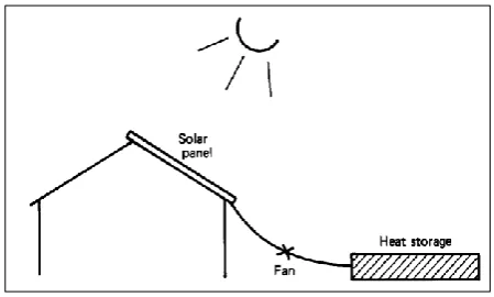
As shown in Figure 2.2, the solar-heated house is considered as an example of a system. The system runs in a way that sun heats the air on the solar panel. The air then flows into heat storage which is a box filled with pebbles. The stored energy can later be transferred to the house. This system is represented in Figure 2.3 and the record of data obtained over fifty hour period and the variables sampled every ten minutes are shown in Figure 2.4 (Ljung, 2012).

Figure 2.2 A solar-heated house. v

y w

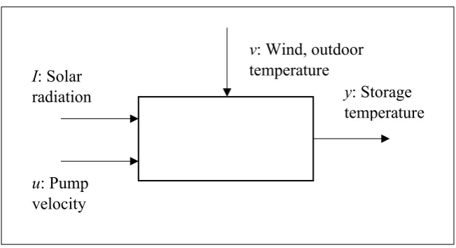
[image:22.595.210.435.503.638.2]

(23)

[image:23.595.159.485.66.243.2]

Figure 2.3 The solar-heated house system: u: input; w: measured disturbance; y: output; v: unmeasured disturbances (Ljung,2012).

(a) Storage temperature (b) Pump Velocity

[image:23.595.122.290.331.442.2]

(c) Solar intensity

Figure 2.4 Storage temperature y, pump velocity u, and solar intensity I over a 50 hour period. Sampling Interval: 10 minutes.

v: Wind, outdoor temperature

y: Storage temperature I: Solar

radiation

(24)

2.1.3 Mathematical Models

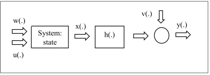
[image:24.595.136.474.193.314.2]

Additive sensor noise term v(.) in Figure 2.5 denote errors produce from the measurement process. W(.) represents input disturbances while a white noise signal, it is usually presumed to represent v(.).

Figure 2.5 Basic structure of mathematical model (Keesman, 2011)

By considering the basic structure of system shown in Figure 2.5, set of standard differential equations with additive sensor noise shown in equation (2.1) and (2.2) as it represent standard description of a finite-dimensional system (Keesman, 2011).

Discrete-time:

𝑥(𝑡 + 1) = 𝑓(𝑡, 𝑥(𝑡), 𝑢(𝑡), 𝑤(𝑡); 𝜗), 𝑥(0) = 𝑥0

𝑦(𝑡) = ℎ(𝑡, 𝑥(𝑡), 𝑢(𝑡); 𝜗) + 𝑣(𝑡), 𝑡 ∈ ℤ+ _(2.1)

Continuous-time:

𝑑𝑥(𝑡)

𝑑𝑡 = 𝑓(𝑡, 𝑥(𝑡), 𝑢(𝑡), 𝑤(𝑡); 𝜗), 𝑥(0) = 𝑥0

𝑦(𝑡) = ℎ(𝑡, 𝑥(𝑡), 𝑢(𝑡); 𝜗) + 𝑣(𝑡), 𝑡 ∈ ℝ (2.2)

Due to the availability of trial data and the ideal modification of a mathematical model into simulation code, the discrete-time form may be apply in system identification while the continuous-time will only be used for demonstration. According to Keesman (2011), these classification also tell the difference between linear and nonlinear, time-invariant and time-varying, static and dynamic systems.

System:

state h(.)

w(.)

u(.)

x(.) y(.)