The Stark effect on helium in the beamfoil source

(1)

THE STARK EFFECT ON HELIUM

IN THE BEAM-FOIL SOURCE

Carl John Sofield

A thesis submitted as a requirement for the degree of

Doctor of Philosophy

at the Australian National University

(2)

(3)

iii

PREFACE

The work reported in this thesis was carried out in the Department of Nuclear Physics at the Australian National University.

I wish to express my gratitude to Dr. H.J. Hay for his supervision. His ability to impart his experience has enriched many discussions and contributed to the solution of many problems encountered during the course of this work.

The low intensity of the beam-foil source necessitated long hours of data collection which were shared with Dr. Hay and my fellow students M.H. Doobov and C.S. Newton. The beam-foil chamber used for the latter part of this work was constructed by C.S. Newton. Part of the computer programme used for the He II data analysis (§6.1) was supplied by M.H. Doobov.

I would like to thank all members of the technical staff in the Department of Nuclear Physics for their efforts in maintaining the

necessary equipment. The skill of Allen Freeman in producing large numbers of very thin carbon foils and maintaining the 2 MeV accelerator is appreciated. I also thank all nuclear physicist members of this department, not only for tolerating "those beam-foilers" on the time-shared computer, but also for their willingness to assist when able.

It is a pleasure to acknowledge the helpful discussions with Dr. L.J. Tassie of the Department of Theoretical Physics.

I am grateful to Prof. Sir E.W. Titterton and Prof. J.O. Newton for allowing me the use of the excellent facilities of this laboratory and to the Australian National University for the scholarship which provided the opportunity to undertake this course.

(4)

Some of the work reported here has appeared in the following publications:

G.W. Carriveau, M.H. Doobov, H.J. Hay, and C.J. Sofield, ’’Reduction of Doppler Broadened Line-widths in Beam-foil Spectroscopy",

flucl. Instr. Meth.

99, 439 (1972).

C.S. Newton, R.J. MacDonald, C.J. Sofield and H.J. Hay,

"Further Evidence Against a Channelling Effect in the Optical Excitation of Ion Beams Transmitted through Single Crystals of Gold".

Pkys. Lett.

42A, 47 (1972).

(5)

V

LIST OF FIGURES

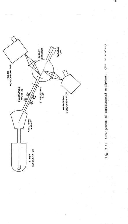
2.1 Arrangement of experimental equipment.

2.2 Horizontal section through cylindrical chamber. 2.3a Intensity of a hydrogen line during life of foil. 2.3b Intensity of a helium line during life of foil. 2.4 Foil damage.

2.5 Relative efficiency of detector system versus wavelength. 2.6 Relative efficiency for polarized light.

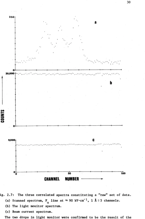
2.7 The three correlated spectra constituting a "raw" set of data.

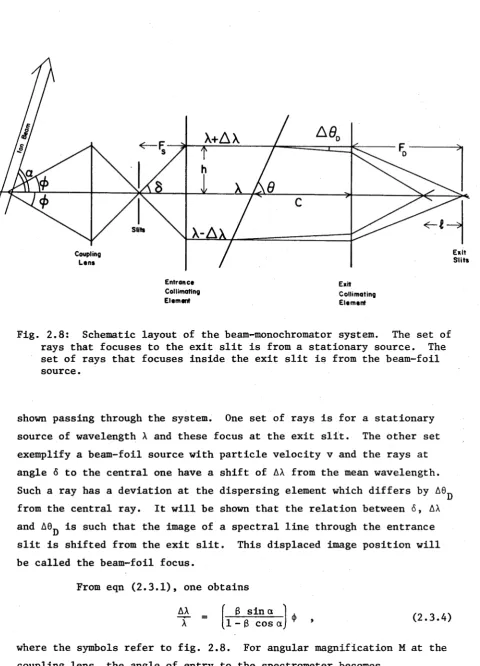
2.8 Schematic layout of the beam-monochromator system. 2.9 Linewidth for stationary source focus and for beam-foil

source focus.

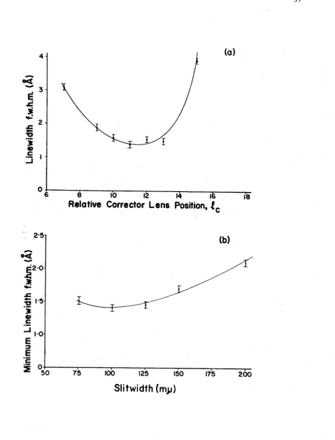
2.10 Experimental re-focusing.

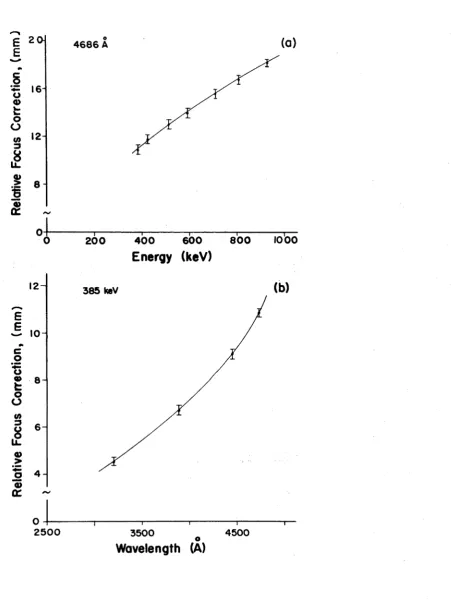
2.11 The variation of re-focused corrector lens position with (a) energy, (b) wavelength.

2.12a Electric field monochromator orientation (a). 2.12b Electric field monochromator orientation (b). 2.12c Electric field monochromator orientation (c). 2.13 Equipotentials from analogue plots.

2.14 Electric field strength along beam axis. 2.15 Resolved Stark components of the H line.

p 3.1 Complete set of data after normalization.

3.2 Improvement of statistical significance from summing data. 3.3 Empirical lineshape.

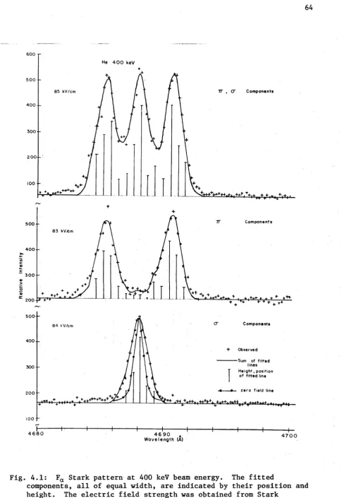
4.1 F^ Stark pattern at 400 keV beam energy. 4.2 F^ Stark pattern at 680 keV beam energy. 4.3 F^ Stark pattern at 820 keV beam energy.

4.4 F^ Stark pattern at 680 keV beam energy and 161 kV«cm- 1 . 4.5 Stark patterns for varying field distributions.

4.6 Calculated Stark splitting of 4 3D-*23P and 4 3F->-23P lines. 4.7 Observed Stark shifts of 4 3D + 2 3P and 4 3F-*23P lines. 4.8 Stark perturbed 4 3D->23P and 4 3F + 2 3P lines for

configuration (a).

(10)

4.9 Stark perturbed 4 3D-*23P and 43F + 2 ' P lines for

configuration (b). 79

4.10 Stark perturbed 4 3D->-23P and 4 3F->2^P lines for

configuration (c). 80

4.11 Wavelength displacement as a function of electric field

strength for 4 3F and 4 3D terms. 84

4.12 Observed Stark effect of singlet lines. 85 4.13 Relative intensities of the singlet Stark components. 86 4.14 Quantum beats observed at varying electric field strengths. 89 6.1 Time evolution model for hydrogenic ions. 105 6.2 Stark pattern as sudden perturbation increases. 108 6.3 Calculated Stark patterns, P and S states. 112 6.4 Calculated Stark patterns, F and D states. 113 6.5 Calculated Stark pattern for statistical initial

population distribution. 114

6.6 Comparison of observed and calculated Stark patterns. 115 6.7 Perturbed lifetimes for the 4 1F31»±1>~2 states. 120 6.8 Decay scheme for the Stark perturbed transitions 4*0 -* 2*P

and 4 1F-*21P. 122

6.9 Electric field distribution and perturbed decay constants. 125 F.l Qualitative evolution of the population of levels in zero

electric field subjected to a "weak field" sudden Stark

perturbation. 165

F.2 Qualitative evolution of the population of levels in zero electric field subjected to a "strong field" sudden

Stark perturbation. 166

F.3 Helium survey scan of the spectral region 4320 Ä to

5300 Ä at 0 kV*cnf1 and 80 kV*cm_1. 167 F.4 Helium survey scan of the spectral region 3000 Ä to

(11)

xi

LIST OF TABLES

4.1 Relative intensities of Stark components at 90 kV*cm_ 1 . 69 4.2 Intensity ratio of fitted Stark components at ±2X to ±5X. 70 4.3 Relative intensities of Stark components at 161 keV*cm_ 1 . 71 4.4 Relative intensities of some He I Stark perturbed lines. 74 4.5 Relative intensities of the 4 3F->-23P components. 81 4.6 Normalized relative intensities of the 4 3D and 4 1F + 2 1P

components. 87

4.7 Quantum beat parameters obtained from the data fitting. 88 6.1 Evolution of the 42S ^ 2 an<* ^2^i/2 P°Pulati°n s *

6.2 Decay factors. 124

6.3 Relative initial populations for 4*D and 4*F excited

states. 127

B. l Transition probabilities and lifetimes. 149

C. l He I singlet eigenvalues. 156

C.2 He I triplet eigenvalues. 157

C.3 He I singlet eigenvectors. 158

C.4 He I singlet transition probabilities. 161

(12)

ABSTRACT

Relative intensities of the Stark components of the He II spectral line (4686 Ä) have been measured following excitation in a beam-foil source, with several beam energies and electric field strengths. Similar measurements have been made for the He I transitions 4 3F->-23P,

+ and 4 1D->21P.

A model of the time evolution of the n = 4 excited states of He II was constructed to include the effects of weak and strong field Stark perturbations. The model selects, from a wide range of postulated initial population distributions, a distribution which is consistent with the observed F^ (n = 4 n = 3 transitions) Stark patterns. It is inferred that the cross-sections for excitation to the n = 4 states decrease as the orbital angular momentum (L) of the excited state increases. For the higher L states, significant alignment, referred to the beam direction, is indicated by a decrease in populations as the z component of the orbital angular momentum (|m |) increases. The alignment was most

pronounced for the 42F term. The energy dependence of the population of n = 4 states was found to be weak for the He beam energy range 400 to 800 keV.

(13)

CHAPTER 1 INTRODUCTION

§1.1 THE BEAM-FOIL SOURCE

The dependence of spectral line intensity on source conditions is a basic reason why new spectral sources may make accessible

information concerning atoms and ions in various states of excitation which is not readily obtained with other sources. It is important to know about the physical conditions and modes of excitation occurring in a particular source in order to utilize the source to greatest advantage. The general features of the source used in this work, a beam-foil source, are outlined below. More comprehensive reports concerning the

properties and applications of the beam-foil source may be found in the

Proceedings of the First, Second and Third International Beam-Foil Conferences [BFS 68, BFS 70, BFS 72].

The beam-foil source [Ka 63, Ba 64] consists of a beam of excited atoms or ions all travelling with nearly the same velocity at a speed which is usually of the order of one per cent of the speed of light. The excitation of the high velocity beam of ions occurs during a very brief interaction with a thin solid foil. The interaction of the ion beam with the foil not only produces ions of different charge states but each charge state has a distribution of excited state populations. The accelerated beam of ions can be produced in a high voltage accelerator of the Van de Graaff type, so the range of elements that can be studied is set by the available ion source. The interaction of the ion beam with the foil may produce ions of high charge states that are not readily obtainable in other sources [Ma 70]. Magnetic mass selection of low current (« 10 yA) beams from an accelerator and high vacuum techniques results in a source of high mass purity and extremely low density. The low density of the beam (« 106 particles•cm"3) gives rise to low emission intensities with consequent experimental difficulties of observing weak spectral lines. The low density of the beam-foil source has the

(14)

electric field from one beam particle at its mean interparticle distance) and the collisional excitation or de-excitation of particles is highly improbable (mean free path % 103 cm). Therefore each particle of the beam is independent of all other particles in the system and can decay only by emission of photons or electrons. The use of molecular beams is thought to lead to space-charge effects if only single exciter foils are used [Se 69].

The high speed of the emitting particles gives large Doppler shifts which may give large broadening of spectral lines because the light is collected over a range of angles governed by the aperture of a spectrometer. Fortunately the beam velocity is nearly uniform which results in a correspondence between Doppler shifted wavelength and the angle of emission such that much of the broadening can be cancelled by a suitable arrangement of experimental equipment.

The nearly uniform velocity of the beam of excited atoms or ions gives a correspondence between the position of observation of radiative decay and the time after excitation that the decay occurs. This feature of the beam-foil source led to its early exploitation for excited state lifetime measurements [Be 65, Wi 70] although difficulties with cascade problems have been common [Oo 70]. Two important properties of the beam-foil source have been discovered more recently; the beam-foil interaction produces coherently excited states and excited state alignment [Ba 66, Ma 69, Se 69, An 70]. Methods of spectroscopic study that rely on alignment of excited states can thus be carried out on the beam-foil source. Zero field quantum beats [Be 72], level crossing

[Ch 71] and magnetic rf resonance [Li 71] techniques have all been applied to the beam-foil source in recent years.

§1.2 BEAM-FOIL EXCITATION MODELS

The beam-foil interaction that leads to the properties outlined above is still not fully understood. A general discussion of the many possible processes involved is given in the Third International Beam-Foil

Conference [BFS 72]. Quantitative theoretical studies [Ya 66, Tr 67, Me 68, Ga 70] are confined to models of the excitation process involving electron capture for hydrogen.

(15)

3

quantum number; individual state cross-sections are not calculated, hence no specific predictions are made with regard to alignment of excited states, although the theory predicts preferential population of states which have a small z component of orbital angular momentum [Me 68, Ha 73]. Experimental evidence has indicated that most of the beam-foil excitation takes place in the last few atomic layers of a foil [Be 70] and is not very sensitive to the mean distance of approach of beam particles and foil atoms [Ne 72], at least for low Z ions. A model put forward by McLelland [Me 68] is applicable to the case of semi-metallic and non-conducting exciter foils where the conduction electron density is low. This model involves the formation of an electron shower by the incident protons and subsequent capture of electrons of a velocity near that of the proton velocity. The energy dependence for the total neutral fraction predicted from this model is in qualitative agreement with

experimental results [Be 72a]. It is of interest in this context to note that Harrison and Lucas [Ha 70], in experiments on proton passage through thin carbon foils, have observed a peak in the ejected secondary electron spectra which corresponds to electrons travelling with velocities near that of the protons. The situation for medium to high Z ions is more complex. The role of inner shell excitation in establishing charge state equilibrium in solid foils has been discussed [Be 70a] in a

semi-quantitative manner, and the contribution to final excited state distributions has been discussed only qualitatively [Bi 70].

§1.3 EXCITED STATE POPULATION DISTRIBUTIONS IN THE BEAM-FOIL SOURCE

The importance of alignment in the methods of spectroscopic measurement previously mentioned makes it desirable to maximize alignment of the ions under investigation. An understanding of the beam-foil

(16)

Several methods of obtaining excited state population

distributions have been applied to the beam-foil source. In the case of one-electron systems the fine-structure cannot be resolved (at least for low Z), so the population distribution among states of different L cannot be obtained directly by intensity measurements as is possible in some other sources [He 56]. However, as the lifetimes of states in one-electron atoms are L dependent the analysis of decay data for a line composed of several transitions from states of differing L value may provide the L state population distribution at the time of excitation

[Do 70]. Difficulties arise with this method due to cascades and coherence [Be 72b], This technique is not possible in multi-electron systems where the transitions of a given multiplet have the same lifetimes [Co 51, p.98].

Observation of polarization of spectral line radiation, in the absence of external perturbations, indicates the existence of alignment in the excited upper level of the transition [Pe 58]. Polarization measurements for spectral lines may provide population distributions for states of the upper level in the transition for the simple transitions n j 1S->n21P» but it does not provide sufficient information to obtain population distributions in more complex cases [K1 69]. Even where

population distributions cannot be obtained from polarization measurements the data is still useful as a qualitative indicator of state population changes for varying excitation conditions [Re 71].

Quantum beat observations have been used to obtain some

relative state occupation numbers in hydrogen and helium [An 70, Do 72]. This method relies on the relation between the amplitude of the quantum beat oscillations and the occupation numbers of the coherently excited states which give rise to the quantum beats [Ma 70a]. Since the

extraction of population distributions from quantum beat measurements is most readily carried out when only a few well separated frequencies

contribute, it becomes very difficult to apply this method to all but the first few excited levels of one-electron atoms [An 70]. Quantum beat measurements in the presence of small magnetic or electric perturbations have been utilized mainly for studies of fine-structure [Ti 73] and the energy shifts caused by the perturbations [An 70a], but these measurements can also be used to obtain information on populations [Se 70]. The

(17)

5

interpret as the number of contributing frequencies increases. A range of quantum beat patterns may be obtained by applying magnetic and/or electric perturbations to the excited ions. The population distributions can be inferred by comparison of these patterns with patterns calculated from postulated population distributions.

In all of the above methods for obtaining populations,

difficulties of interpretation increase as the number of degenerate or near degenerate states increases for the initial level of interest. It

is well known that strong magnetic and electric fields remove all or part of the degeneracy occurring in an excited level of an ion thus giving rise to a pattern of separated spectral lines, the Zeeman or Stark patterns respectively [So 72, pp.263-285]. The application of static magnetic fields to a high velocity charged particle beam results in a motional electric field [Wi 16] and hence a combination of magnetic and electric perturbations on the ions; for this reason static electric fields are simpler in their effects.

§1.4 THE STARK EFFECT

The effect of an external electric field, the Stark effect, on ions has been known for 60 years. The application of the early quantum theory to explain the phenomena [Ep 16, Sc 16] was one of the earliest successes of this theory. The solution of the Stark effect perturbation problem has been revised and updated as atomic physics progressed,

providing an interesting historical development of atomic physics. A review of the Stark effect and its measurement has been made by Bonch-Bruevich and Kodovoi [Bo 67].

The perturbation to the Hamiltonian of an ion in a uniform electric field, F, directed along the z-axis is -eFz (where e is the absolute value of the electronic charge 1.6><10-19 C) . The matrix elements of the perturbation are proportional to the dipole matrix elements for radiative transitions so that only states of the same term system (AS = 0), opposite parity (AL = ±1), and the same z component of total angular momentum (AM^ =0) are coupled. The perturbation possesses cylindrical symmetry about the z-axis and hence removes any degeneracy of the system except that associated with the sign of M^.

(18)

different L value and the same principal quantum number, and a quadratic Stark effect when the shifts are smaller than the separations.

For Stark effect problems involving terms with fine-structure it is useful to distinguish between field strengths that give rise to energy shifts less than the fine-structure separation (weak fields) and greater than the fine-structure separation (strong fields). The actual magnitudes of strong or weak fields therefore depend on the ion and spectral term being considered, and there is, of course, an intermediate region. The usefulness of this distinction arises because the total angular momentum is approximately conserved (i.e. J is a good quantum number) for weak fields, whereas in strong fields the uncoupling of the orbital and spin angular momenta result in the z component of the orbital angular momentum M and the spin angular momentum Mg being separately conserved so that J is no longer a good quantum number but M = M + M q is. Hence, for weak fields the electron spin may be treated by calculating the Stark effect of the fine-structure and for strong fields by treating the fine-structure of the Stark effect.

In very weak fields the dipole selection rules for J and are the same as for zero field, namely A J = 0 , ± 1 (J = 0 = 0) , AM =0,±1

J

(Mj = 0-^Mj = 0 for AJ = 0) . The strong field Stark components (defined as transitions from levels of given |m |) may have fine-structure, and they obey the dipole selection rules AM =0, with AM = 0 (tt polarized

components), or A M = ± 1 (a polarized components). However, L is a good quantum number only for vanishing electric fields. Hence dipole

radiative decay channels occur that are forbidden at zero field. In the case of the Stark effect of He I the appearance of the resultant

forbidden spectra lines is striking and so also is the removal of metastability of the 22S^ states of hydrogenic ions.

§1.4.1 The First-Order Stark Effect

Neglecting spin, the first-order Stark effect for hydrogenic ions may be solved using non-degenerate perturbation theory. This is done using parabolic co-ordinates because in that system the perturbed Hamiltonian matrix is diagonal [Fo 62]. The energy levels of a

hydrogenic ion in an electric field are given by, _ _ mZ2e4 3Fh2 ,

(19)

7

where m is the mass of an electron, Z the atomic number, n the principal quantum number, nj and n 2 are the parabolic or electric quantum numbers, and

n = n 1 + n 2 + | M | + l . (1.2) The wavelength of a Stark component arising from a transition between the two states (n,n1,n2,M) and (nT ,nj,n2,M*), where the primes indicate the lower level, is shifted from the zero field wavelength by

AX , — C , F , (1.3)

nn nn

where

c ,

nn

.n_, n 4 n' 4 Xn n ’

- 5.3169x10 (n 2 - n * 2) 2 z 5 » (1.4)

and

X ,

nn = n(nj - n 2) - n ' f a j - n j ) , (1.5) for AX ,

nn in Ä and F in kV«cm-1. Notice that the wavelength shifts are integer multiples of the displacement for X , =1. There may be more than one transition with the same displacement aX ( a = 0,±1,±2,±3, ...), these being distinguishable if they have different polarizations. This treatment neglects spin so it is only valid for strong fields where the relative displacement of components is given accurately by eqn (1.3). If the Stark components are resolved eqn (1.3) may be used to determine the electric field strength F.

There is a quasi-selection rule which says that transitions in which the sign of (nj - n 2) differs from the sign of (nj - n 2) will be very weak [Be 57, pp.231, 276]. Consequently most of the highly displaced components are "unobservably" weak.

§1.4.2 The Second-Order Stark Effect

In multi-electron ions the electron-electron interaction

removes the L degeneracy characteristic of one-electron ions and therefore there is no first-order Stark effect. The correction to the energy of a Stark perturbed state is, to second order,

ctJM. F2 2 a ’ J'

|<aJM I e 2 z. | a ’J'M )|2

EaJ Ea ’J f

(

1. 6)

(20)

particular cases. The denominator, E T - E tTt, in eqn (1.6) dominates a J a J

the magnitude of the level shift and gives rise to the familiar

repulsion of coupled states. For the lowest terms of multi-electron ions where E ^ - E ^ , ^ , is large the Stark effect is negligible up to high field

strengths (e.g. « 1 cm-1 at 535 kV«cm_1 for the 2 ^ ^ state of He I). This results in the perturbation of the upper term dominating the wave length shift of the Stark perturbed transitions. The Stark components arising from transitions (AM=0,±1) between highly excited terms and the first few slightly perturbed terms are both ir and a polarized if the lower term has a state of the same M value as the upper term, otherwise only a o polarized component occurs.

§1.5 POPULATION OF EXCITED STATES AND THE RELATIVE INTENSITIES OF STARK COMPONENTS

The detected intensity K ^ of a Stark component resulting from a dipole transition from state i to state k may be expressed as

X ik = K ik l< 1 lp lk > l2 «i . (1-7)

where K ^ is a constant dependent on the volume of emitting ions, the frequency of the radiation, the direction and solid angle of observation and the wavelength and polarization efficiencies of the detector, and P is the electric dipole operator. If the intensity of a transition from i to k relative to that for i to k, the relative values of K., and K.. , and

lk j k the dipole matrix elements for the transitions are known, then the ratio of the populations N^ and N_. can be found from eqn (1.7). Thus it is necessary to know the Stark perturbed dipole matrix elements to determine the relative populations of Stark perturbed states from relative

intensity measurements. The populations are indeterminate to the extent of the Mj degeneracy. If the Stark components have unresolved fine-structure, a further indeterminacy in populations results.

For hydrogenic ions, the dipole matrix elements of the strong field Stark components are equal and field independent [Ho 65] for components symmetrically displaced about the wavelength of the

(21)

9

Since the interatomic electric fields are much larger than the fields applied to the beam outside the foil, the excitation processes which occur in the foil populate states which are not the Stark states at the point of observation. In order to deduce features of the excitation process, a relationship between the relative populations of the Stark states and the relative populations of the initial states excited in the foil must be obtained. Specifying this relation is in essence a problem of calculating the time dependence of the excited state populations and the coherence terms between these states. The particular time dependence of the problem is determined by the very short time in which excitation occurs in the foil (giving a time origin) and the approximate

correspondence between position and the time after excitation due to the nearly uniform velocity of the beam of excited ions. The static electric fields applied to the beam are seen by the high velocity excited ions as time varying electric fields, and therefore time dependent Stark

perturbation effects must be accounted for. These time dependent perturbation calculations reduce to simple forms in the case of the sudden, adiabatic, and the resonant time dependent approximations.

A model of the time evolution process embodying the relation of the initial excited state populations to the relative intensities of Stark perturbed transitions has been constructed. The model includes calculations of the change in populations with time due to radiative decay, coherence effects and perturbations. The model is formulated in the density matrix representation to facilitate the calculation of

coherence effects and because the relative populations of excited states are averages over the ensemble of excited ions. For input, the model requires the measured relative intensities of Stark components and values of the Stark perturbed transition probabilities and lifetimes. The use of the model is thus restricted to ions for which the Stark effect perturbation problem has been solved.

The early observations by Bashkin and Carriveau on the Stark effect in a beam-foil source [Ba 70] were of interest in that, although individual Stark components were not resolved, the lines in hydorgen, H D

(22)

from the high field ionization of long wavelength components [La 31] or the preferential collision quenching of low wavelength components [Ge 68], but neither of these effects could contribute significantly under the experimental conditions of Bashkin and Carriveau. The possible

contribution of excitation or perturbation induced coherence to the observed asymmetry was not considered. The time dependence of the applied electric field was implied to be infinitely slow.

§1.6 SCOPE OF THE PRESENT WORK

This thesis is concerned with strong field Stark effect

observations using beam-foil excited 4He+ ions obtained from a 2 MeV Van de Graaff accelerator. The passage of the ions through the foil produces neutral, singly ionized and doubly ionized 4He particles providing the He I and He II spectra for study. The choice of 4He allowed the study of the quadratic (He I) and the linear (He II) Stark effects for spectra where theoretical and experimental information on perturbed transition probabilities and Stark perturbed energy level values are available [Lii 51, Ku 73, Fo 28, Pf 66], without extra complications due to the necessity of including hyperfine-structure. The theoretical information was necessary in order to relate the measured Stark relative intensities to the initial populations of excited states. The eigenvalue problem for the linear Stark effect including spin is treated in Appendix B, where the perturbed transition probabilities and lifetimes for strong fields are also given. In Appendix C, the eigenvalue problem for the Stark effect in He I is presented and perturbed transition probabilities and lifetimes for field strengths up to 100 kV«cm-1 are tabulated.

To obtain reliable relative intensity measurements of Stark components at strong fields, considerable development of experimental methods was required. The intensity of transitions from He I and He II were found to decrease the higher the excitation of the upper level. The

Stark effect measurements were carried out on some terms of principal quantum number n = 4 for this reason. The largest separation of Stark components at 100 kV*cm_1 was about 2 Ä. The linewidth achieved for spectral lines was approximately 1 Ä (F.W.H.M.) so that some Stark

(23)

11

(24)

CHAPTER 2 EXPERIMENTAL EQUIPMENT AND METHODS

The equipment used for the Stark component intensity measure ments from the beam-foil source falls into three classes. These are apparatus constituting the beam-foil source, that used to measure relative intensities free of the influence of source fluctuations, and that required to obtain resolved Stark components. The latter class involves the attainment of strong uniform electric fields and the

improvement of spectral resolution by cancelling the major component of Doppler broadening. The design and use of these combine to determine the success with which the relative intensities can be obtained. Some of the general features of the way in which experimental considerations interact are given before the details of the equipment are discussed.

The strength of the electric field applied to the excited ion beam determines the separation of the Stark components. The electric field strength depends on the electrode design, the beam-foil chamber design and vacuum pressure and the high voltage supplies. The presence of the high energy ion beam and the secondary electrons resulting from

its impact on the foil and collimator edges make the achievement of constant electric fields difficult.

The Doppler broadened linewidths of « 10 Ä for He spectral lines at about 800 keV beam energy precludes the resolutions of Stark components separated by ^ 1 Ä. The attainment of such Stark splitting often requires uniform electric fields in excess of 100 kV*cm_ 1 . Methods of cancelling the major component of Doppler broadening were investigated and the method of re-focusing the monochromator was found to be the best one for strong field Stark effect measurements. The factors limiting the achievable linewidth obtained with a re-focused monochromator were

considered. The sensitivity of the re-focusing to beam velocity and wavelength changes had to be investigated in order to establish

satisfactory procedures for Stark effect observations. This was necessary because the electric field produces changes in the wavelength of the

(25)

13

The measurement of relative intensities also depends, apart from resolution considerations, on the source intensity, the methods of light collection, and signal processing. The variation of the source efficiency with time was investigated and necessitated monitoring both the beam current and the light intensity from a chosen transition. The effective use of the monitor information was greatly facilitated by the use of digital data acquisition techniques because on-line arithmetic procedures allowed corrective action to be taken before changes in conditions became large enough to lead to the collection of unreliable data.

§2.1 BEAM-FOIL SOURCE EQUIPMENT

The equipment necessary to establish a beam-foil source is found in most low energy nuclear physics laboratories where charged particle accelerators are used. The energy range and ion source of the accelerator determine the range of isotopes, charge states, and the spectral range that may be studied. Source efficiency variations may arise in the accelerator ion beam output or from changes in the exciter foil due to bombardment. Separate monitoring of beam current and a spectral line allowed these two sources of variation to be distinguished.

§2.1.1 Accelerator and Beam-Line

A schematic diagram of the accelerator and beam-line is given in fig. 2.1. The diagram indicates typical positions for a Heath

monochromator used to monitor the source light output, a McPherson scanning monochromator used to obtain the spectra of interest, and the Faraday cup used to monitor beam current.

The accelerator was an H.V.E.C. Model AK, 2 MeV Van de Graaff equipped with an r.f. ion source. The 22.5° analyzing magnet (mass

energy product 36) bends the accelerated beam into the beam-line where it then passes through a quadrupole lens, stabilizing slits and collimator before passing through a thin foil in a chamber where electric fields could be established and observations could be made. The pressure maintained in the accelerator and beam-line was less than 10"5 torr.

§2.1.2 Beam-Foil Chambers

(26)

[image:26.539.81.525.38.811.2]

(27)

15

cylindrical chamber of 15 cm internal diameter and 20 cm high,

constructed from mild steel and cadmium plated. A section in the plane of the beam is given in fig. 2.2. The beam path was 75 mm below the top of the chamber. Three 4.1 cm diameter fused quartz observation windows were provided, two cutting the plane of the beam centred on a horizontal diameter perpendicular to the beam axis, and one in the centre of the chamber lid.

The chamber was equipped with a foil wheel which had 22 holes, each 4 mm in diameter. This was mounted so that the hole at the top of the wheel intersected the beam axis. Rotation of the foil wheel from outside the chamber was accomplished by a manually operated worm drive through a rotating vacuum seal. The foils were mounted on tantalum frames (0.4 mm thick with 4 mm diameter holes) which were glued to the foil wheel.

Two insulated electrodes made from automotive spark plugs were mounted on the chamber on a circle 5.2 cm in diameter, spaced 7.3 cm apart and equally spaced from the beam to provide high voltage

leadthroughs.

Earthed aluminium plates 2.5 mm thick, 4 mm apart at the beam axis, with 2.5 mm diameter apertures to allow beam passage, were

suspended from the chamber lid. These baffles served to shield the foil and the light monitor.

The stabilizing slits (1 to 2 mm gap) and the 1.5 mm aperture at the chamber entrance 4.5 cm from the foil restricted the beam

divergence to approximately 0.008 rad. The beam diameter at the chamber centre, measured by charring a cardboard target, was approximately 1.5mm. The beam divergence was kept small to reduce its contribution to line broadening.

The chamber was pumped by a liquid nitrogen trapped oil

diffusion pump mounted below the chamber and separated from it by a flap valve. The chamber pressure was monitored by an ionization gauge

situated at the end of the Faraday cup. The pressure indicated at that position was always less than 10"5 torr when experiments were in progress.

The second beam-foil chamber was considerably larger,

(28)

CO a) 0

X ) cd

o <U u PQ u u • 01 CJ fH CU

x r H 1—1•H

cu O

•H Ph

PH •

• co

• pH X

w DO 3

• O

• r H P4

u 0) x <u 0) 4-1

X JG X

0 G

G CU

rG r H rH

o •H

O X )

r H pH CU cd 4-1 o • G

•H & r H Jh 3

x CO

G • G

•H CU •H

r H r H X 4-1 CU O 4 4 DO CO G

-G X 4-4 DO r H

G 4-1 O O j d > S-i Ö0

X •H X

4-1 r H DO

•H

G X PC

O C

•H G • 4-1 X

CJ CO <U CU CO x •

O CO

r—1 p4 CU

cd 4-1 p4

4-1 O 3

G CU 4-1

o rH p4

N CU cu

•H a

U X ) G

O CU

PC x DO

4-1 G

V-I •H

• » G G

CN PC •H

• 4H CN • _CU

CJ X

(29)

17

held 60 foils, was rotated by a stepping motor. The insulated high

voltage electrodes were brought through the chamber lid 13.5 cm apart and equally spaced about the beam. An earthed stainless steel plate 3 mm thick was suspended from the lid of the chamber 10 mm from the foil wheel and had a 2.5 mm diameter aperture at the beam axis. The beam divergence was about the same as that for the other chamber. Observation ports extended over about 43 cm on both sides of the chamber parallel to the beam axis.

The stray magnetic field in the chambers was measured with a Hall probe and found to be < 0.1 G. This field had no observable effects on the beam-foil source lines since the resultant Zeeman splitting of a Lorentz triplet is approximately 10 5 cm 1. The motional electric field

(« 1 V-cm_1) for a singly charged ion of ß «s 0.02 is also negligible.

§2.1.3 Changes in Foils Under Beam Bombardment

The foils used were thin self-supporting carbon foils produced locally by evaporation onto glass slides coated with RBS 25 detergent. The foils were subsequently floated off with distilled water and picked up on the tantalum foil holders. Thin foils were required in order to reduce the Doppler broadening of spectral lines resulting from scattering. Foil thicknesses were between 2 and 7 yg'cnf 2 . The thickness, within this range, was not critical provided the variation between foils of a set was small. The similarity of thickness was estimated visually by the optical transmission of the carbon film on the glass slides. Measurement of a particle energy loss through two thicknesses of foil showed that the thinnest self-supporting foils which could be handled easily were

2.5 ±0 . 5 yg'cm-2 thick.

The excitation efficiency of the foils was found to be time and beam current dependent. A steady decrease in light output was sometimes observed before the more drastic reduction when a foil broke. The time taken for a foil to break was less for heavier ions and for higher beam currents, but no clear relationship was established.

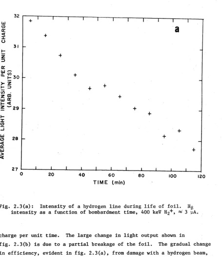
The variations with time of the relative intensity measured by the Heath monitoring monochromator, for the H line of hydrogen and the

p

3 3p-*23S line of He I are shown in fig. 2.3(a) and fig. 2.3(b)

(30)

T I M E (min)

Fig. 2.3(a): Intensity of a hydrogen line during life of foil. Hg intensity as a function of bombardment time, 400 keV H2+ , *** 3 yA.

charge per unit time. The large change in light output shown in

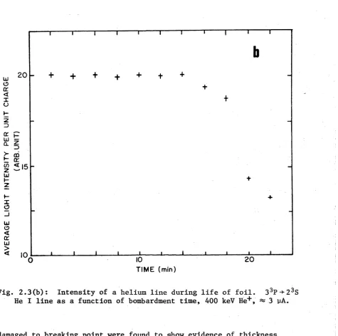
fig. 2.3(b) is due to a partial breakage of the foil. The gradual change in efficiency, evident in fig. 2.3(a), from damage with a hydrogen beam, was also evident with He+ beams at lower beam currents (ss 1 y A ) . The slow change in efficiency with time of bombardment by a hydrogen beam was a general feature due to damage of the foil and was not due to breaks large enough to detect visually. While the Heath monitored the 3 3P-*23S He I line for the data of fig. 2.3(b), the McPherson monochromator

simultaneously observed the 4 3D-*23P He I line. The ratio of these two signals remained constant within counting statistics until the foil broke.

[image:30.539.52.508.58.585.2]

(31)

19

TIME (min)

Fig. 2.3(b): Intensity of a helium line during life of foil. 3 3P ^ 2 3S He I line as a function of bombardment time, 400 keV He+ , « 3 yA.

damaged to breaking point were found to show evidence of thickness

changes in the regions subjected to beam damage. The changes appeared as thick areas, % 500 Ä in diameter randomly distributed through « 50% of the foil.

[image:31.539.56.532.69.541.2]

(32)

z

D er Hi

CL

a

> CO

H

h-CO 7

2 d

LlI

z ®_{- or} <i h- — X

S£

hj

_J o a: LlI <

O I

< O a:

LU > <

2

o

o o

o

+ +

o

+

E 5 X h-9 £

LlI

2

3+

2

*

1 "

r i i i I

i

0 +

o

₅₀

₁₀₀

₁₅₀

T I M E (min)

Fig. 2.4: Foil damage. (a) Hg relative intensity per 400 keV H 2+ , 3 yA, as a function of time. (b) Hß function of time, monochromator slits set at 125 ym, instrumental linewidth of « 1 Ä.

(33)

21

carbon build-up from cracked oil vapours does not appear to account for the increase in thickness.

The combination of light and current monitors served to

indicate whether foil damage was extensive enough to affect significantly the width of spectral lines during the time taken to scan over the wave length range of the Stark spectra. The monitoring procedure became important from this point of view because the scattering in the foils, which is thickness dependent, was a major component of the linewidth after the Doppler broadening from the finite aperture collection optics was cancelled. This was especially so for incompletely resolved Stark components, because data fitting procedures which relied on linewidth estimates from zero field observations prior to obtaining the Stark

spectra, were used to obtain the relative intensities of such components.

§2.2 EQUIPMENT FOR RELATIVE INTENSITY MEASUREMENT

The instrument used for relative intensity measurement was a scanning monochromator with a photomultiplier detector operating in the photon counting mode. To compare source emission intensities, the

overall dependence of the system's detection efficiency on wavelength was measured, as was also its dependence on polarization. The efficiency of

the photocathode and grating, as well as the transmission of the various lenses and chamber window contributed to the system's efficiency.

§2.2.1 Scanning Monochromator

A McPherson 218 scanning monochromator was used to obtain spectra from the region of the beam where electric fields were applied. This instrument has a focal length of 0.3 m, aperture ratio f/5.3 and is based on a crossed Czerny-Turner design to reduce off-axis aberrations at the collimating mirrors and to allow efficient baffling against stray light. The plane-grating used with it had 2400 £*mm-1 and was blazed for 3000 Ä. The reciprocal linear dispersion in first order was about 12 to 8 Ä«mm- 1 over the grating’s wavelength range of 1800 Ä to 5300 Ä giving about 0.2 Ä linewidth when the slits were set at 20 ym. The grating was driven by a constant speed motor through a gearbox.

(34)

wavelength onto the entrance slit. Unit magnification was used to obtain maximum transfer of light from the beam [Ca 70].

A thin linear polarizer (Polaroid HN22) could be inserted in a rotatable holder just before the entrance slit of the monochromator. The grating reflected light polarized parallel to its rulings less than light polarized perpendicular to them. The beam, electric field, and

monochromator orientations (§2.3.4) were such that the relative efficiencies for light polarized in those directions was required.

The instrument was modified by the addition of a lens just inside the exit slit to allow it to be re-focused (§2.3.3) for the beam-foil source. Absorption in the glass lens reduced the wavelength range to 3000 Ä to 5300 Ä.

The monochromator was also modified by the addition of a cam to the wavelength drive train to operate a microswitch at 10 & intervals. The microswitch permitted the synchronization of the monochromators,

scalers and computer which were used for data collection. The micro switch operation was reproducible to within ±0.03 Ä. The differential linearity of the wavelength scale is important; for example a 2% change in electric field strength may give rise to a shift sufficient to change the deduced Stark component intensity by 10%, but for these Stark effect measurements the absolute zero of the wavelength scale does not matter.

For use with the cylindrical chamber the monochromator was mounted on wooden slides to provide motion approximately perpendicular and parallel to the beam. With the stainless steel chamber it was

mounted on rigid metal plates driven by accurate lead screws. The slides were used to position the monochromator at each wavelength so that the source was focused at the entrance slit and to position it up and down stream to view between the field electrodes for the Stark effect

measurements. The splitting of the H line was measured to find the p

region of maximum field strength.

(35)

23

0- —

3000 5000

WAVELENGTH (A)

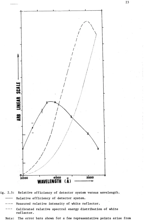
Fig. 2.5: Relative efficiency of detector system versus wavelength. ---- Relative efficiency of detector system.

---- Measured relative intensity of white reflector.

•••• Calibrated relative spectral energy distribution of white reflector.

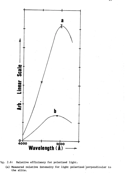
[image:35.539.53.532.48.776.2]

(36)

The relative intensity of the reflectance standard was also measured with the linear polarizer inserted with its polarization axis first parallel and then perpendicular to the slits. Fig. 2.6 shows the reflector relative intensity as a function of wavelength for the detector system with the polarizer inserted. The Stark perturbed transitions were observed in the wavelength range 4680 ± 20 Ä for which interval the ratio of efficiency for light polarized perpendicular to the slits to that polarized parallel to the slits was 3.6±0.2. The transmission through the polarizer was 39 ± 2% for that wavelength range. These measurements allowed the relative intensities of it components and o components,

obtained with electric field monochromator orientation (a) (§2.4.2), to be corrected for grating efficiency.

Over a 40 Ä range, which exceeds the Stark splitting of the F^ (4686 Ä) line, the change in overall efficiency is about 4%, which gives a very small correction to the Stark component intensities. The wavelength dependence of the detector efficiency must be allowed for when comparing the intensities of widely separated spectral lines.

§2.2.2 Monitoring Monochromator

A Heath EUE-700 scanning monochromator was used as a light monitor. It has a single-pass Czerny-Turner configuration with aperture ratio f/6.8 and a focal length of 0.35 m. This instrument is equipped with a 1180 £ *mm 1 grating giving a nominal reciprocal linear dispersion of 20 Ä*mm 1 in first order. The resolution is better than 0.5 Ä over its usable range of 1900 Ä to 1 ym. The monitor was normally operated with entrance and exit slits at 2000 ym, giving a 40 Ä pass band in order to obtain maximum intensity from the Doppler broadened beam-foil lines.

(37)

25

4000

Wavelength (A)

Fig. 2.6: Relative efficiency for polarized light.

(a) Measured relative intensity for light polarized perpendicular to the slits.

(b) Measured relative intensity for light polarized parallel to the slits.

Note: The source intensity is the same for both measurements. The error bars shown for the few representative points arise from

[image:37.539.53.533.47.708.2]

(38)

§2.2.3 Single-Photon Counting

E.M.I. 6256S photomultipliers were used as detectors with both monochromators. These phototubes had fused quartz windows and "S" type photocathodes of 10 ram diameter.

The phototubes were mounted in housings that enabled the tubes to be operated at low temperatures («* -AO °C) and thus reduce dark

current noise. The housing was a modified version of the one developed by Carriveau [Ca 70]. It consisted of an outer brass cylinder separated from a copper cylinder by a V thick insulating poly-urethane foam. The end of the copper cylinder adjacent to the exit slit was closed by an annular copper coil with a 10 mm diameter open hole at its centre. The phototube projected into this cylinder with the cathode close to but not touching the coil. Dry nitrogen, boiled from liquid, was re-cooled in a heat exchanger immersed in liquid nitrogen close to the housing, and blown onto the photocathode. An insulating nylon tube pierced the earthed brass enclosure to deliver the cooled gas to the copper coil. Dark count rates of 0.5 to 1 count»s-1 were obtained in this way.

A further separate compartment at the end of the brass cylinder contained the voltage divider network for the photomultiplier dynode chain. The voltage divider was constructed to give good performance under single-photon counting conditions [Za xx ] . The voltage divider was operated with the anode at ground potential and was coupled to a Fluke 3 kV power supply. A further separate compartment housed a direct-coupled, non-overloading, fast pulse preamplifier (rise time < 10 ns, duration < 30 ns). These were built locally following a design of Jackson's [Ja 65].

The low level pulses from the preamplifier were passed through an ORTEC 410 linear amplifier, with no pulse shaping, to an ORTEC 420 single-channel analyzer operated as an integral discriminator. The threshold of the single-channel analyzer was raised sufficiently to eliminate the low level noise.

(39)

27

and 2000 V a t 200 V i n t e r v a l s . At low v o lt a g e s th e p h o to tu b e g a in b a r e l y

overcam e t h e p r e a m p l i f i e r n o is e b u t th e tu b e s i g n a l - t o - n o i s e r a t i o was

h ig h . At h ig h v o l t a g e s th e c o u n tin g r a t e was much h i g h e r , b u t th e

s i g n a l - t o - n o i s e r a t i o was lo w e r. F or low l e v e l c o u n tin g , c h a r a c t e r i s t i c

o f b e a m - f o il s o u r c e s , t h e e f f e c t i v e a c c u ra c y in th e l i g h t s i g n a l

m easu rem en ts d ep en d s n o t o n ly on th e s i g n a l - t o - n o i s e r a t i o b u t a l s o on

t h e a b s o l u t e c o u n tin g r a t e . H ence, d ep en d in g on th e lo w er l e v e l o f

s i g n a l s one w an ts to d e t e c t , th e w orking tu b e v o l t a g e and d i s c r i m i n a t o r

l e v e l n eed t o be ch o sen t o g iv e maximum s i g n i f i c a n c e to t h e s i g n a l c o u n t

o b ta in e d i n a g iv e n tim e .

D e f in in g th e s i g n a l - t o - n o i s e r a t i o a s R = S/B g iv e s

T = (R + 1)B , (2 . 2 . 1)

w here T and B a r e th e t o t a l r a t e s e s tim a te d from Bj c o u n ts i n tim e t i and

T2 c o u n ts i n t 2 . Then t h e s i g n a l in t 2 i s

and t h e e r r o r in S2 i s

S2 T2 - Bj (2 . 2 . 2)

E = /( R + l ) B1 ( t 2/ t i ) + ( t 2 / t i ) /bT . ( 2 .2 . 3 )

To s i m p l i f y th e d i s c u s s i o n , su p p o se t 2 = t i = t , th e n

E = /ß ( A + R + 1) ( 2 .2 .4 a )

o r

E = / s ( / l + 1/R + 1 //R ) . ( 2 .2 .4 b )

I f R << 1 , th e n E « 2/b, t h a t i s th e r e l a t i v e e r r o r i s

E » 2 / / P b . ( 2 .2 . 5 )

K

I f R > > 1 , t h e e r r o r i n S i s sim p ly / s . Between t h e s e l i m i t s th e r e l a t i v e

e r r o r i n S , w here S now i s th e s i g n a l c o u n tin g r a t e , i s

E„

= l//stT

( A

+ 1/R + l/v^R) .

K

The r e l a t i o n s h i p b etw een th e r e l a t i v e e r r o r , th e s i g n a l - t o -

n o i s e r a t i o , and t h e sa m p lin g tim e can be seen by two e x am p les. The

f i r s t exam ple i s , i f t h e s i g n a l and back grou n d c o u n t r a t e s b o th d o u b le

th e n th e s i g n a l - t o - n o i s e r a t i o re m a in s th e same so E i s re d u c e d by /2 o r

a l t e r n a t i v e l y th e same a c c u r a c y can be o b ta in e d in h a l f th e tim e . F or

th e seco n d ex am p le, c o n s id e r w hat happens i f th e b ack g ro u n d r a t e

(40)

doubles, so R halves. Then

Er = 1/Sst (/l72 + 1/R + l/»/R) .

Notice that although the signal-to-noise ratio has worsened the relative error has decreased, that is the accuracy with which the signal can be measured has improved by an amount depending on R.

Looking now at eqn (2.2.5), for small R, as long as B increases no faster than the square of the increase in S, the accuracy achievable

for S in a given time increases even though the signal-to-noise ratio decreases.

By making use of the above principles the optimum tube voltage was found to be 1300 V, some 200 to 300 V lower than would normally have been chosen for operation in the analogue current measuring mode with high signal-to-noise ratio. An increase in the tube voltage of 100 V was found to increase the signal count rate by 10%, but the dark count rate by 25% to 30% for signal-to-noise ratio in the region of 1 to 10. The signal-to-noise ratio did increase as the discriminator level was raised, but the sacrifice in signal count rate made the time required to obtain the same statistical significance too long to make this increase in signal-to-noise ratio an improvement.

§2.2.4 Data Recording

After processing by the single-channel analyzers, the signals from the two monochromators became ORTEC standard logic pulses (5 V, 500 ns) suitable for driving scalers. Two other sources of logic pulses were from the beam current collected in the Faraday cup and processed by an ORTEC 439 Current Digitizer, and a regular train of clock pulses at a rate of 100 s ~ 1. These signals were connected to a block of four

computer controlled scalers.

The microswitch on the scanning monochromator activated the clock and provided a command signal to the laboratory’s IBM 1800 computer which then collected counts in each scaler for a nominated time, read the

The Stark effect on helium in the beamfoil source