Linear programming and the calculation of maximum norm approximations

· ?I.AR1$

LINEAR PROGRAMMING AND THE CALCULATION OF MAXIMUM NORM APPROXIMATIONS

by

DAVID H. ANDERSON

A thesis submitted to the Australian National University for the degree of Doctor of Philosophy.

Acknowledgements Preface

Abstract

CHAPTER 1: I NTRODUCTI ON

CHAPTER 2: BEST LINEAR CHEBYSHEV APPROXIMATION 2.1 INTRODUCTI ON

2.2 CHARACTERIZATION

2.3 DISCRETE LINEAR CHEBYSHEV APPROXIMATION CHAPTER 3: NUMERICAL DETERMINATION OF BEST LINEAR

CHEBYSHEV APPROXIMATIONS 3.1 INTRODUCTION

3.2 ALGORITHMS

CHAPTER 4: APPROXIMATE SOLUTION OF DIFFERENTIAL EQUATIONS 4.1 MINIMAX RESIDUAL SOLUTION OF OPERATOR

EQUATIONS

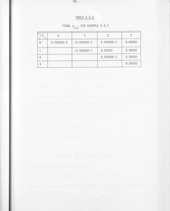
4.2 LINEAR ELLIPTIC PARTIAL DIFFERENTIAL EQUATIONS

CHAPTER 5: NON-LINEAR PROBLEMS

5. 1 A DESCENT METHOD FOR MINIMIZING I~(:) II 5.2 A LEVENBERG-LIKE METHOD

5.3 CONTINUOUS NON-LINEAR BEST APPROXIMATION

i i iii

9 9 15 22

27 28 31 54

56

CHAPTER 6:

REFERENCES APPENDIX I

AN EFFICIENT ALGORITHM FOR DISCRETE NON-LINEAR BEST APPROXIMATION

6.1 A FULL-STEP METHOD 6.2 MAXIMIZING EFFICIENCY

6.3 NUMERICAL RESULTS AND DISCUSSION

This work was carried out at the Computer Centre, Australian

National University. I wish to thank the head of the (entre, Mike Osborne, for his supervision and general support. His suggestions concerning the presentation of this thesis have also been most welcome.

I would also like to thank Bob Anderssen and Richard Brent for many encouraging and stimulating discussions. Thanks are also due to Bernie Omodei for his help in checking the typescript, to Mike Saunders for providing a listing of an early version of his linear programming routines, and to Greg Woodford for providing the contour plotting routines used in preparing the diagrams in Chapter 3. The skill and patience of the typists, Mrs Anne Clugston, and Mrs Jenny Hinchey, is obvious from the typescript and to them I owe my gratitude.

Without the financial assistance of an Australian National University postgraduate scholarship, this thesis would not have been possible.

i i

PREFACE

Many of the results in this thesis have been established or were greatly improved by discussion with Dr Mike Osborne. The work of Chapter 6 stemmed from a series of lectures given by Dr Richard Brent of the Computer Centre, on his paper (Brent [15]). Discussions with Dr Brent have led to a number of improvements in this Chapter. This thesis makes use of a number of results in the field of linear

programming. The standard reference is Hadley [28]. The use of stable implementations of the simplex method was suggested by Mike Osborne after a visit to Stanford University, California, where he learned of the work of Dr Mike Saunders. The routines given in Appendix Iare based on some

originally written by Dr Saunders for Dr Osborne. Dr Saunders visited this University on a number of occasions and discussions were carried out with him on the development of the linear programming algorithm.

J

ABSTRACT

This thesis examines methods for the solution of a number of approximation problems which include multivariate approximation and the approximate solution of differential equations. After a brief discussion of the literature in Chapter 1, the best linear Chebyshev approximation problem is discussed in Chapter 2. A brief introduction to the general theory is given, which includes a number of characterization theorems. The discrete linear Chebyshev approximation problem is then discussed and it is shown how this may be solved by linear programming techniques.

In Chapter 3, the problem of determining, numerically, best linear Chebyshev approximations is considered, and two algorithms are given. Chapter 4 generalizes the methods of Chapters 2 and 3 to enable the numerical calculation of approximate solutions of differential equations to be made. A method is developed which can be used when the

approximating family does not satisfy the boundary conditions. In §4.2 linear elliptic partial differential equations are considered in detail, and an error bound is derived. Use can be made of this to produce an approximation with the best error bound.

Non-linear problems are considered in Chapters 5 and 6. In §5.3,

two methods are presented for non-linear continuous approximation which I are analogues of the methods of Chapter 3. The methods depend on an

algorithm for the solution of a discrete problem. Two such algorithms are presented in §5.l, §5.2. In Chapter 6, an investigation is made into the question of improving the efficiency of these algorithms. An

algorithm is presented which is similar to those of Chapter 5, and which depends on a parameter, k. Conditions are given under which the

iv

CHAPTER 1

INTRODUCTION

Let GeRm be a bounded domain, and consider the problem of finding an approximate solution of the (possibly non-linear) operator equation

~ u = f in G.

The method of approximation considered in this thesis involves the determination of an element,

u

,

from a suitably chosen set of approx-imations such that

is minimized. The norm,

II· "

_G, is a generalization of the usual maximum (Loo) norm, defined such that

Ilfll

_G = _x max _{€ G} If(x)1 _{_}

This choice is particularly suitable whenever error estimates of the form

can be derived, where K is some constant. Such estimates are available, for example, for certain elliptic partial differential equations, (see Schryer [62J, for instance).

An advantage of the maximum norm over other norms occurs in the solution of non-linear problems. For example, consider the problem of minimizing \tJith respect to ~, the function

F(x) = II!(~)IIG'

where f is a vector function of x. This problem occurs as a subproblem

-in the calculation of non-l-inear approximations (see §5.3). Under

2.

that the order of convergence is at least two. The corresponding method

for the least squares norm has, in general, only first order convergence.

Moreover, Kowalik and Osborne [32 ] have shown it can be divergent fr6m

a point arbitrarily close to the solution.

Further advantages of the maximum norm can be found in the text

of this thesis, where a number of algorithms are able to make explicit

use of the linear programming formulation of the solution procedures to

greatly improve the algorithms. For example, a generalization of the

first algorithm of Remes (see Chapter 3) can be computed in a particularly

efficient manner.

Chapters 2 and 3 deal with the usual linear approximation problem

in which M is just the identity operator, and the norm

II

·

II

G

is the usual

maximum norm. Approximations,

u,

are sought in the form

n

u

_L

i=l

where the ~. are suitably chosen functions, defined on G. The main

1.-aim has been to develop an algorithm capable of solving approximation

problems in more than one dimension. This is important as it enables

generalization to the approximate solution of partial differential

equations.

The method of approximation considered in Chapter 3 is to solve

a sequence of discrete problems on finite subsets Gk of G using a

general-ization of the first algorithm of Remes. It is shown in §2.3 that the

discrete problems may be formulated as linear programming problems.

An alternative algorithm for solving the discrete problems was

given by Lawson (see Rice and Usow [55

J).

Use is made of the fact that

the solution of the discrete problem is also' the solution of a certain

functions {<Pi} form a Chebyshev set (see §2.l). Mairhuber [37J (see also, Theorem 2.1.4) has shown that Chebyshev sets exist only on very special higher dimensional spaces, and hence this assumption is too restrictive. Furthermore, the method involves solving a sequence of weighted least squares problems, so that the linear programming

approach should be more efficient. It is not clear whether the method still works for the continuous case.

A different method which is capable of solving the continuous problem in higher dimensions has recently been given by Fletcher, Grant and Hebden [ 22 J. The method is based on a suggestion by P6lya [49 J in connection with polynomial approximation and depends upon considering an Loo approximation as the limit as P ~ 00 of LP approximations, where

Ilf

I~

Difficulties with the P6lya algorithm may arise both through the size 00 •

of P required to obtain a satisfactory estimate of the L Solutlon, and through the subproblems for determining the successive LP approximations. Some of the latter difficulties have been overcome through the authors' implementation of an algorithm for solving LP problems (see Fletcher, Grant and Hebden [23J). The question of the size of p, however, is more difficult, and the above authors have had some success in character-izing the asymptotic behaviour of the LP solutions so that extrapolation procedures may be used. A draw-back with their method, however, is that the calculation of the LP approximations is difficult and may be quite time consuming on a computer. Moreover, the integrals involved must be calculated numerically, which re-introduces the discrete problem.

A descent method for the continuous problem has been given by

4.

The linear programming method is more general and is easily implemented. It can also cope readily with arbitrarily shaped domains (see, for example, Barrodale and Young [5

J).

The special case of Loo approximation by multi-dimensional splines has been investigated by Schultz [ 63J and by Rosen [58 J. The work of Schultz is mainly of a theoretical nature, while Rosen's main contribution is in providing estimates for the difference between the uniform error over the whole of G, and the discrete error over a finite point set,for an approximation computed on the finite set. Such estimates are not

considered in this thesis as the proposed method is capable of approaching arbitrarily closely an approximation with minimum uniform error.

A multiple exchange algorithm for multi-variate Loo approximation has been given by Watson [69

J.

The algorithms considered in this thesis use .only single exchanges but they can be easily extended to use multiple exchanges. Our approach differs from that of Watson in that he advocates finding the local extrema of the error curve

n

L

i=l

k

a. <p. (x)

1.- 1.-

-k

r(a , x) = f(x)

at the k-th step by Newton's method applied to the problem of finding

the zeros of IJ _ r(a_ k, _ x), starting from the "reference points", {F,;-1.-.} C Gk . The n+l reference points where the current maximum value of the error function is attained are identified by the columns in the final basis of the dual formulation of the linear programming problem. However, to ensure convergence of the algorithm it is necessary to extend Watson's definition of reference points to include all of the points of Gk at which the maximum error is attained. If only those points determined by the optimal basis matrix are used, then Watson's proposed algorithm may not converge to the correct solution if two or more of the points

the sense of Osborne and Watson [46

J.

A search would thus be necessary to locate the reference points.

The approach used in §3.2 is to search at each step, for a point

xk for which the error is greater than any value on the set Gk. It is believed that this method will lead to a good approximation in a shorter time than Watson's algorithm, although no numerical comparisons are available.

Chapter 4 generalizes the concept of best Loo approximations to deal with the approximate solution of linear differential equations. Various

approximation methods are discussed, depending on whether a family of approximations can be found satisfying the differential equation on the boundary conditions, or neither. The main contribution is in developing a method that can be used when the approximation satisfies neither differential equation or boundary conditions. This is important because it allows the use of general approximating families. For example, product

B-splines (see Rosen [58

J)

can be used without the need for the boundary conditions to be satisfied. This is particularly advantageous in

domains of general shape, or when the boundary conditions are complicated. In §4.2 linear elliptic partial differential equations are

considered in detail and an error bound is derived, use of which can be made to produce an approximate solution,

u

,

with the best error bound. Rosen [58

J

also considers an extension to the approximate solution of certain linear boundary-value problems. His main concern, there, however, is to investigate problems for which his error bounds and computational method for approximating functions can be applied with a

minimum of difficulty. For this reason, he restricts consideration to

problems defined by linear differential operators with polynomial coefficients.

Elliptic boundary-value problems have also been considered by

6.

differential boundary conditions has been given by Cheung [18

J.

The

approach in these papers is different from the one in this thesis in that

the above authors use a fixed grid of discrete points and then derive

error estimates valid over the whole domain, G, which can be obtained by

solving an associated linear programming problem. In this thesis, use

is made of the much simpler error bound given in §4.2 and the generalized

first algorithm of Remes to produce an approximation with the best

uniform error bound.

The above authors also consider quasi-linear problems to which

their methods may be extended. The method of Chapter 4 may likewise

be extended, using an error bound derived by Schryer [62

J,

although this

extension has not been included here.

Non-linear Loo approximation problems have been considered by a

number of authors (see, for example, Rice [53, 54J, Dunham [21 J). However,

most of the literature deals with exponential and rational approximation

(see, for example, Braess [12,13,14]' Rice [51 J, Lee and Roberts [34J),

Few general methods are available. In §5.3 two methods are presented

for non-linear continuous approximation which are analogues of the methods

of Chapter 3. The methods require the solution of a sequence of discrete

problems which can be considered as special cases of the more general

problem :

fi nd x € Rn to

where f(x) is a vector function of x, and the norm is the usual £00

vector norm, defined by

\\ u _{_}

\I

= m~x _-z.. \ u _-z.. .\

For this reason, special attention i~ given in §5.1 and §5.2 to

methods for the solution of this general problem. In §5.1 a method

a zero of a vector function of several variables (see, for example,

Ortega and Rheinboldt [42

J).

A similar algorithm has been considered

by Osborne and Watson [45

J.

however, their method requires a

one-dimensional minimization to be made at each step. In §5.1 , a number

of assumptions are given which ensure that the sequence {x.} generated

-t.

by the algorithm converges. Further assumptions are given to ensure

the algorithm has second order convergence.

An alternative algorithm is given in §5.2 which is analogous to

a method proposed by Levenberg [35

J,

Marquardt [38

J

and Morrison [41

J

for the least squares solution of the problem. More recently, Madsen

[36

J

has considered a similar algorithm to the one given here. However,

our treatment is more general and we introduce a number of parameters

which may be adjusted to improve the convergence of the algorithm.

Moreover, the formulation in §5.2 allows the question of order of

convergence to be considered. The method is exceedingly general and

requires fewer assumptions to ensure convergence than does the algorithm

of §5.1.

Both of the above methods require the solution of discrete

linear Loo problems at each step, and the linear programming method of

§2.3 is used for their solution.

In Chapter 6, an investigation is made into the question of

improving the efficiency of the algorithms of Chapter 5, where efficiency

is a measure of the total work required to compute the solution of an

iterative procedure. An algorithm is presented which is similar to

those of Chapter 5 and which depends on a parameter, k. It is shown

that under essentially the same conditions as used in §5.1 , the algorithm

has an order of convergence of at least k+l. It is then shown how k

may be chosen to maximize efficiency.

Because many of the algorithms in this thesis require the solution

of discrete Loo

8.

is included in the appendix. The code is written to take advantage of

the special structure of these problems. Some introductory material is

CHAPTER 2

BEST LINEAR CHEBYSHEV APPROXIMATION

2.1 INTRODUCTION

Let X be a compact subset of ~ with metric d and let C[X] denote the space of all continuous real-valued functions on X with norm

(2.1.1)

This is the maximum (or Chebyshev) norm. If there is no ambiguity, we

will often use

II

fll

instead of

II

fll

X·

Consider the problem of approximating a function fE C[X] by a

linear combination of some prescribed functions ~1' ... , ~P E C[X].

Let

P

F(Ct,x)

= l: Ct. ~ .(x)

- - i=1 ~

~-(2.1.2)

where Ct =

(

Ct

1

,

... ,

Ctp

)T

E RP, and define the residual function

r(Ct,x) =

f

(x) -

F

(

Ct

,X)

(2.1.3)

The best linear Chebyshev (BLC) problem is to find a vector Ct E RP to

minimize

II

r(~,~)

Ilx'

The existence of solutions to this problem is

guaranteed by the following theorem.

Theorem 2.1.1 Riesz [ 56 ]

A finite dimensional linear subspace of a normed linear space

contains at least one point of minimum distance from a fixed point. 0

We cannot, however, ensure uniqueness without imposing an

additional assumption on the functions ~.(x). This assumption is that ~

-the set {~.(x)} is a Chebyshev set.

-10.

Definition 2.1.1

A set of functions {cj>l' ... , cj> } is said to be a Chebyshev set

. p

on X if and only if each determinant

(2.1.4)

is non-zero for any p distinct points ~l' ... , ~p € X.

An equivalent definition can be formulated in terms of the number of zeros of F(a,x) in X.

Theorem 2.1.2

A necessary and sufficient condition that {cj>l' ... , cj>p} be a

Chebyshev set on X is that no non-trivial expression of the form (2.1.2) have more than p-l distinct zeros in X.

Proof

Let the set {cj>l' there are p zeros, ~l'

, cj> } be a Chebyshev set. Suppose that

p

,x of F(a,x) for some a. Then we have

-p - -

-F(a,x_{_ -1-}.) = 0, (i = l~ ... ~ p) .

This can be expressed in matrix notation as

o

(2.1.5)

where A = (a . . ), a . . = cj> .(x.) . 1-~ J 1-~ J 1--J

(2.1.6)

The determinant (2.1.4) is non-zero, since {cj>l' ... , cj>p} is a Chebyshev set, by assumption. Therefore, A is non-singular and so

Conversely, suppose no non-trivial expression of the form (2.1.2) has more than p-l distinct zeros. Let ~l' ... , ~p be any p distinct points in X and construct the matrix (2.1.6). By assumption,

T

A a

t

0 for all a

to.

It is a standard result of linear algebra that A is non-singular and hence the determinant (2.1.4) is non-zero. See, for example Collatz

o

[19, p.91]. This proves sufficiency.

The fundamental theorem concerning uniqueness of BLC approxima-tions was proved by Haar [ 27].

Theorem 2.1.3 Haar [ 27]

Every function f E C[X] possesses a unique best linear Chebyshev approximation of the fonn (2.1 .2) if and only if {CP1' ... , cpp} is a

Chebyshev set.

o

Proofs of this theorem may be found in Achieser [1, p. 67] , Cheney [17, p.80], and Meinardus [39, p.16].

Chebyshev sets {CP1' ... , cpp} do not exist on all compact metric spaces if p ~ 2. This is clear, for if ~l' . .. , ~p are distinct

points of an open sphere SCXc~, m > 2~ then ~l and ~2 may interchange their positions in X, keeping ~3' ... , ~p fixed, by a continuous

simultaneous motion in S such that xl' ... ,x remain distinct. The

- -p

result of this interchange is to change the sign of the determinant

(2.1.4). Therefore, the determinant must have vanished for some intermediate ~l and ~2 so that {CP1' ... , cpp} is not a Chebyshev set.

12.

Theorem 2.1.4 Mairhuber [.37 ]

A compact metric space XCRm, containing at least p points, may .

serve as the domain of definition of a non-trivial (p ~ 2) Chebyshev

, ~ } of functions if and only if X is homeomorphic to a

p

closed subset of the circumference of a circle. o

The absence of Chebyshev sets on arbitrary metric spaces means

that uniqueness of the best linear Chebyshev approximation cannot be

guaranteed. This is not usually a serious problem as often any

solu-tipn will suffice. Of much greater importance is the calculation of

the BLC approximation. This question will be considered in a later

section. In the special case where X is a finite interval [a,b] we can

strengthen the result of Theorem 2.1.2 by distinguishing between two

types of zeros, nodal and non-nodal zeros, (Karlin and Studden

[29 , p.22]).

Definition 2.1.2

For any continuous function

f(x

)

on [a,b] an isolated zero

Xo € (a,b) of f is said to be a non-nodal zero provided the function

f does not change sign at xo' All other zeros, including zeros at the

end points a and b, are said to be nodal zeros.

Theorem 2.1.5 Karlin and Studden [29, p.23]

Let {~l' .,. , ~p} be a Chebyshev set on a fi nite i nterva 1 [a,b]. Then no non-trivial expression of the form (2.1.2) has more then p-l zeros on [a,b] where nodal zeros are counted once and non-nodal zeros twice.

Proof

Assume {~l' ... , ~p} is a Chebyshev set on [a,b] and let

{x., i = l~ ... ~ r} be the nodal zeros and let {y o , j == l~ ... ~ s} be

~ J

the non-nodal zeros. Define a. to be the sign of F(Ct,x) near y.. By

J J

Theorem ?.l .2, r+s ~ p~l . Define the additional points

k == l~

.

..

~ q == p-r-s}

It follows from the assumption that {~l' ... , ~p} is a Chebyshev set

that there is a S such that

F(S,x.) =0, (i==l~ ... ~r)

-

~

F(S,y.)= a .~ (j==l~ ~s)

- J J

and F(~,zk) = 0, (k == l~ ..• ~ q)

Define

a

= Ct -

£S.

Clearly, for £ >

°

sufficiently small, F(~,X) will have two zeros near

each y. and one zero at each x .. Therefore, F(~,x) has r+2s zeros. By

J ~

Theorem 2.1.2, r+2s ~ p-l, which is the desired result.

An alternative proof of the above theorem may be found in Karlin and

Studden [29, p.23].

Example 2.1.1

a) {l, x, x2 } is a Chebyshev set on [a,b] for any a,b since the

Vandermonde determinant

1

X 2

1

X 22 = (x 2 - x_l )( x.3 - x_l )( x.3 - x 2 )

X 2

.3

which clearly cannot vanish if xl' _{x2' x.3} are distinct.

14.

b) {1, X2, X4} is a Chebyshev set on [a,b] if ab > 0 but not if

ab < O. This follows since

1

1 X 2

;5

X 4 1

X 4 ;5

The determinant will therefore be non-zero for distinct xl' X₂' x;5 if

and only if two of the points have opposite signs.

c) {l, (x-a)2} is not a Chebyshev set on [O,b], 0< a < b,since the

2.2 CHARACTERIZATION

Definition 2.2.1

Let r{a,x) be as defined in §2.1. A point x e X with

(2.2.1)

is called an extremal point of r{~,~).

Theorem 2.2.1 Kolmogoroff [ 30 ]

A necessary and sufficient condition that F{a,x) be a best

approximation to

f

{x)

is that

min {r{a,x) ( )} 0

xeD • F S,x : (2.2.2)

for all S e RP, where D is the set of extremal points of r{~,~).

Proof

This is a slightly simplified version of a proof given in

Meinardus [ 39 ].

Let (2.2.2) be satisfied for all S e RP. If F{a,x) is not a best

approximation, there exists a S such that

(2.2.3)

Now, for all xeD,

r{a,x) F{a -S,x) = r{a,x)[F{a,x) - F(S,X)]

= r{a,x)[r(a,x) - r(S,x)]

2

~

II

d~,~)

II

-

II

r{~,~)

II

16.

Since D is compact,

min {r(a,x) . F{a -S,x)} > 0

. xeD -

-which is a contradiction. This proves sufficiency.

Conversely, suppose F{a,x) is a best approximation but (2.2.2) is not satisfied for all S € RP. Then there exists S e RP such that

-0

min ( ) ( )

D {r a,x . F S ,x }

= a

> 0 . xe _ _ -0

-Clearly, an open subset, U, of X can be chosen so that DCU and

Then

Now, let ~ = ~ + Y§o so that

and hence

or

F{S,X) = F{a3x) + y F{S ,x)

-0

-r{S,x) = r{a,x) - y F{S ,x) -0

-In U we have, using (2.2.4), (2.2.7)

2 2 2

1r(~,~)1 < 1r(~,~)1 - ya + y211 F{~o,~) llx

provided y ~ O.

Clearly, for sufficiently small y > 0

In X-U we have, using (2.2.5), (2.2.6)

(2.2.4)

(2.2.5)

(2.2.6)

{2.2.7}

(2.2.9)

for sufficiently small y.

Combining (2.2.8), (2.2.9) we obtain

which is a contradiction. This proves necessity.

o

The characterization theorem just proved can be stated in an

equivalent form.

Theorem 2.2.2 Cheney [17, p.160]

A necessary and sufficient condition for F(a,x) to be a best

approximation to f(x) on X is that there exist points x. _{_t.} € X and scalars

A.

t

0 such that

t.

and (i i)

Lemma 2.2.1

L: A.cp .(X.) = 0, (j = 1~ ... ~ p). i t. J _t.

If F(a,x) is a best approximation to f(x) on X and if

o

{CP1' ••• , cpp} is a Chebyshev set on X then the set 0 of extremal

points of r(a,x) contains at least p+l points provided X contains at

least p+l points.

Proof

If 0 contains p, or fewer, points there exists a 8 € ~ such that

18.

Also, r(a.,x)

t

0, X € D. (2.2.11 )

Otherwise r(a.,x) == 0,

so that D would contain more than p points. From (2.2.10), (2.2.11) we

deduce that

r(a.,x) F(S,x) = r2(a.,x) > 0 (2.2.12)

for all x € D. By Theorem 2.2.1, this contradicts the assumption that

F(a.,X) is a best approximation to

f

(x).

Therefore, D contains at least

p+l points. 0

It can happen that D contains fewer than p+l points. An example

is provided by the approximation of x2 by

0./

+ a.₂

l

over 0 < x < 2 (see Curtis and Powell [20 J, Osborne and Watson [46J). The best

approximation is given by (to eight figures)

0.18423193

0.41863139

II

r(<;:,~)

II

~ 0.53824532

There are only two extremal points. One of these is x = 2 and the other

is the root of the equation

which is (to eight figures)

x 0.40637574.

Definition 2.2.2

Let F(a.,X) be a best approximation to f(~) on

X.

If the set D

of extremal points of r(a.,x) contains fewer than p+l points then the

Lemma 2.2.1 shows that if {~1' ... , ~p} is a Chebyshev set

then the BLC problem cannot be singular if X contains at least p+1 points. We now consider an important special case. Let X be the real

interval [a,b], a < b. If {~1' ... , ~p} is a Chebyshev set on [a,b]

then the characterization of BLC approximations can be given in a much more convenient form.

Theorem 2.2.3 Chebyshev [ 16], de la Vallee Poussin [ 68 ]

Let {~1' ... , ~p} c C[a,b] be a Chebyshev set on [a,b]. In

order that

F

(

a

,x)

shall be a best approximation on [a,b] to a given f € C[a,b] it is necessary and sufficient that there exist at least p+1 points a < x < x

- 1 2 ... < x p+l -< b such that r(a,x) satisfies

(i)

Ir(a.) x .) I

=

II r(~,x) II , (i = 1.) , p+l)

- t.

and (i i) r(a,x.) + r(a,x. 1)

=

- t. - t.+ 0, (i = 1, , p).

If r(a,x) satisfies (i) and (ii) then it is said to alternate

p+1 times.

Proof

Let us assume that

F

(

a

,x)

is a best approximation to f but

r(~,x) does not alternate at least p+1 times. By Lemma 2.2.1, the set, 0, of extremal points of r (a,x) contains at least p+1 points. There are at least two of these points at which r(~,x) has different signs. We can assume that t.. = II r(~,x) II > 0 since otherwise

20.

with m < p such that either

or

r(a,x) > -~ for x €[a'~l]

r(a,x) < ~ for x €[~2'~3]

r(a,x) < ~ for x €[a'~l]

r(a,x) > -~ for x €[~1'~2]

(2.2.13)

(2.2.14)

We restrict attention to (2.2.13). The proof for (2.2.14) follows

similarly. Let 0 be the smallest number in D. There are two cases.

1. Suppose k = p-m-l is even. Then we choose k distinct points n· J sufficiently close to (but not equal to) a zero of r(a,x) such that

I

r (a, n .)

I

~ ~ ~~ (j = 1 ~ ... ~ k) .

- J

(2.2.15)

Since {<P

l , ... , <Pp} is a Chebyshev set, there exists a (unique) vector

S such that

F(~'~l) = 0,

(

i

= l~ ~

m)

F(S,n.) = 0, (j = l~ ... ~ k)

- J

and F(S,o) = sign (r (a,o))

Using Theorem 2.1.5 we deduce that

r(a,x)F(S,x) > 0 for x € 0 . (2.2.16)

By Theorem 2.2.1 this contradicts the assumption that F(a,x) is a best

approximation to

f

.

2. Suppose k = p-m-2 is even. Then we choose k points n. as above.

J

F(8,t.;.) = _{0, (i}

₌

₁₎

_m)

~ 1-

...

,

F(8,n .) = 0, (j

=

1,

...

k)

~ J )

F(8,o) = sign (r(a,~)) and F( 8, r;) = sign _(r(a,I'J) where l; ~ b is the largest number in D.

Again using Theorem 2.1.5 we deduce that

r(a~ ,x)F(8~ ,x) > 0 for xeD (2.2.17)

which again contradicts the assumption that F(a,x) is a best approxima-tion to f. This proves necessity.

To prove sufficiency, assume that r(a,x) alternates p+l times on {xl' ... , x_p+₁} but F(~,X) is not a best approximation to f . Then, by Theorem 2.2.1 there is a 8 such that

r(a,x)F(8,x) > 0 for all xeD. Since x. e D we must have

1-sign(F(~,xi)) = -sign(F(~,xi+l))'

(i = 1, ... , p).

(2.2.18)

This implies F(8,x) has p zeros in [a,bJ. Using Theorem 2.1 .2 we

22.

2.3 DISCRETE LINEAR CHEBYSHEV APPROXIMATION

If {q,1' ... , q,p} is a Chebyshev set and if the positions of the

extrema of r(a,x) are known, the BLC approximation can be calculated by solving a linear system of equations. The location of these extrema, however, usually involves the solution of some non-linear equations.

In any case, Chebyshev sets do not exist in more than one dimension (see Theorem 2.1.4). Therefore, various approximate methods are

used, the simplest of which consists of selecting a finite subset Y in X and then solving the approximation on Y instead of X. This is the discrete linear Chebyshev (DLC) approximation problem, and it can

be written:

find

(2.3.1 )

mi nimi ze

This problem can be formulated as:

find a € RP and h € R to

minimize h

subject to the constraints

Let Y = {~1' ... x } and define the matrix F and vector f such -n

that

F . . = q,.(x.), (i=l~ ... ~ pj j=l~ ... ~ n)

1.-~J 1.--J (2.3.2)

and f.=f(x.), (j=1~

J -J ~ n). (2.3.3)

Then, the above problem can be written as a linear programming (LP) problem:

a € RP~

find h € R to

minimize h

where e denotes the vector each component of which is unity. This may be written

find

[~]

€ RP+1 to

minimize Z =

[~T,l][~J

subject

(2.3.4)

which is a standard form for LP problems. Note that it is not necessary to include the constraint h > 0 because any solution of

(2.3.4) automatically satisfies h : O. The above formulation requires the addition of 2n "surplus variables" and a may not be constrained in sign. Both of these problems can be overcome by solving the dual

problem:

find w € R2n to

maximize z =

subject to _{w =}

[~J

(2.3.5)

and w > 0

The solution of problem (2.3.4) is given by

(2.3.6)

where n* is the vector of Lagrange multipliers at the optimum of the dual problem (see Appendix I).

The problem (2.3.5) can be solved using a modification of the Revised Simplex Method which takes advantage of the special structure of the problem (see Appendix I). The particular implementation used

24.

iteration and so n* is available at no extra cost.

The classical results concerning the solution of this problem are

based on the assumption that the matrix F satisfies the Haar condition.

Definition 2.3.1

If every pxp submatrix of F is nonsingular, F is said to

satisfy the Haar condition.

The following result follows immediately from the definition.

Remark 2.3.1

The matrix F defined by (2.3.2) satisfies the Haar condition if

and only if the set of functions {~1' , ~p} is a Chebyshev set on

Y. A sufficient condition for {~1' ... , ~p} to be a Chebyshev set on

Y is that it be a Chebyshev set on X-:JY.

An exchange algorithm for solving the problem (2.3.l) was given

by Stiefel [ 66

J.

A sufficient condition for convergence of the

algorithm is that F satisfy the Haar condition. Osborne and Watson

[ 47

J

pointed out the equivalence of the Stiefel exchange algorithm

and the linear programming method of solution.

Theorem 2.3.1 Osborne and Watson [ 47

J

The Stiefel exchange algorithm is equivalent to the Simplex

Method of linear programming applied to the dual formulation (2.3.5)

of the OLe approximation problem. 0

The Haar condition was not used in the proof of equivalence.

All that was required was the non-singularity of the successive basis

matrices. For this we require that the matrix

in (2.3.5) have rank p+l. It is sufficient that F have rank p. This is clearly much weaker than the Haar condition.

An algorithm for solving the OLC approximation problem was given

by Lawson (see Rice and Usow [ 55 ]). Use is made of the fact that the solution of the OLC problem is also the solution of a certain weighted

least squares problem. However, it is necessary to assume the

func-tions {¢1' ... , ¢p} are a Chebyshev set. Furthermore, the method

involves solving a. sequence of weighted least squares problems so that the linear programming approach should be more efficient, although no

numerical comparisons are available.

Lemma 2.3.1

If a column of the matrix (2.3.7) is in the optimal dual basis

then the corresponding inequality in the constraints (2.3.4) holds as

a strict equality.

Proof

The proof follows directly from complementary slackness results

of linear programming (see, for example, Hadley [28, p.239]). o

Remark 2.3.2

It is a consequence of the linear programming formulation that there are at least p+l points ~i such that Ir(~v'~i)1 = II r(~v'~) I~ provided rank (F) = p. This follows from Lemma 2.3.1 since there are

p+l columns in the optimal dual basis. If two vectors

[r]

and

LiJ

appear in the dual basis then II r(~v'~) Ilv = 0 so that

r(a

_-

v'x.) = 0 for all x. € V.

-~ -~

An advantage of the linear programming "formulation is that a

26.

capability is not possessed by the Stiefel exchange algorithm. A

program for implementing the Simplex Method for solving OLe problems is

given by Barrodale and Young [ 4

J,

however their method is based on

the usual Simplex Method which uses Gauss-Jordan elimination to update

the inverses of the basis matrices.

It has been known in numerical linear algebra for over twenty

years that inverting matrices by using Gaussian elimination without

suitably choosing the pivots is numerically unstable. By this is

meant that if a matrix is to be inverted on a computer, which

represents each number to a finite number of digits only, then

Gaussian elimination without choice of pivots may lead to large errors

in the inverse.

A computationally stable implementation of the Stiefel exchange

algorithm has been given by Bartels and Golub [ 7

J who use a

technique based on LU decomposition with row interchanges.

The linear programming method is, however, more widely

applic-able and if the LP code is suitably modified, the storage requirements

are comparable. Numerically stable implementations of the Simplex

Method have been given by Bartels and Golub [ 8

J,

Bartels [ 6

J,

Bartels, Stoer and Zenger [ 9

J,

Gill and Murray [26

J

and Saunders

[59, 60, 61J.

The numerical results in this thesis were computed using an

algorithm based on the method of Saunders. An advantage of Saunders'

method is that it was designed for large, sparse LP matrices and it

may be possible to take advantage of his method for approximation using

CHAPTER 3

NUMERICAL DETERMINATION OF BEST LINEAR CHEBYSHEV APPROXIMATIONS

This chapter deals with computational schemes for determining

BLC approximations. In §3.l we show that BLC approximations may be

computed by using finer and finer discrete sets, Y. This has obvious

disadvantages. An" alternative is to use the first algorithm of Remes,

however this involves finding global extrema of multimodal functions.

An alternative algorithm is presented in §3.2 and the convergence is

proved. The remainder of §3.2 deals with various results concerning

the algorithm. Specifically, we show how use can be made of the

line~r programming formulation to compute the sequence of BLC problems

generated by our algorithm. We also prove conditions under which only

one additional Simplex iteration will be sufficient to solve the

successive BLC problems. Finally, we indicate how the algorithm may

be improved and we give a numerical example to illustrate the algorithm

28.

3.1 INTRODUCTION

If the set Y defined in §2.3 somehow fills out the metric space

X, we expect the discrete approximation to be "close" to the true

(continuous) approximation on X. It is possible to make this intuitive

idea more rigorous.

De fin it ion 3. 1 . 1

The density of Y in X is denoted by

!Y! = max _{xeX yeY} inf d{x ) _,y'

where d is the metric in X (see §2.1).

We have the following theorem.

Theorem 3.1.1 Cheney [17, p.86]

(3.1.1)

Let X be a compact metric space and f> <P

1> ••• > <Pp e C[X]. For

each yeX let F{~y'~) be a best approximation to

f{x)

on Y of the form

(2.1.2). If F{~X'~) is a best approximation to f{~) on X, then

as !y! + 0, where r{a,x) is defined by (2.1.3). o

To ensure the discrete approximations F{~y'~) converge to

F{~X':) we require the uniqueness of F(~X'~)' for which it is sufficient

that {<P

1, ... ,<pp} be a Chebyshev set (see Theorem 2.1.3) .

Theorem 3.1.2 Cheney [17, p.87]

Let X be a compact metric space and f> <P

1, .. , , <Pp elements of

C[X]. If

f

(

x)

possesses a unique best approximation F(~X'~) on X, then

its best approximations F(~y'~) on subsets Y £onverge to F(~X'~) as

One consequence of the above results is that computation of a

BLC approximation can be carried out by computing OLC approximations

on finer and finer discrete sets. However, to obtain a good

approx-imation it may be necessary to use a large number of points in Y. The

matrix F would therefore be large, which could cause difficulties when

solving such problems on a computer.

Remes (see Cheney [ 17 ]) presented two algorith~which

over-come this difficulty. The second algorithm of Remes makes explicit

use of the alternation property (see §2.2) and so it is necessary to

assume {<P

l , ... , <Pp} is a Chebyshev set (see Theorem 2.2.3). The

first algorithm of Remes is more generally applicable since it is not

necessary that {<P

l ,

...

,

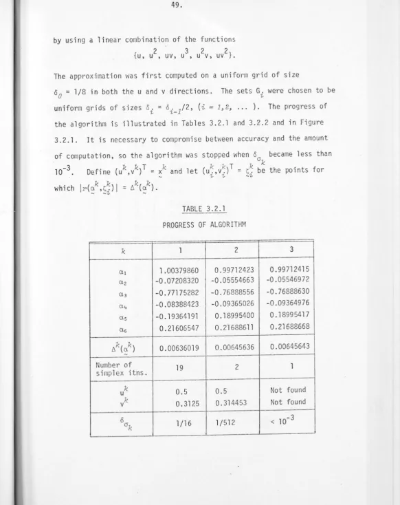
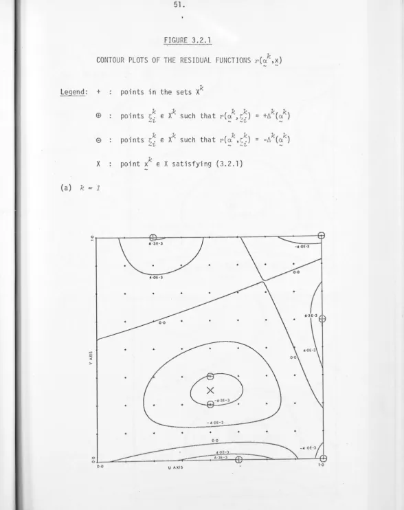
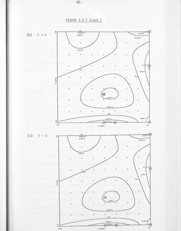
<P } p be a Chebyshev set. It

solution of a sequence of discrete problems on finite

where Ixkl does not

and

tend to zero. For convenience

6(a)

=

II r(~,:) II X

6k(a) = II

r

(

~

,:)

II X k .

we

requires the

subsets

X

k

of X,

define

(3.1.2)

(3.1.3)

The set of functions {<P

l , ... , <Pp} is assumed to be independent. (If it is not it can be replaced by a smaller set that is independent

without increasing the minimum 6(a).)

The First Algorithm of Remes (see Cheney [17, p.96])

At the k-th step we are given a finite subset

Xk

of X. Select

ak to minimize the function 6k(a). Choose xk € X to maximize

Ir(~k,~)

I·

Set Xk+l = Xk U {xk} and continue.

At the beginning Xl may be arbitrary except that the matrix F

defined by (2.3.2), where Y = Xl, should be of rank p. It follows from the assumption of the linear independence of the <Pi on X that this

30.

One difficulty with this method is the calculation of the points xk that maximize

Ir(~k,~)

I.

These points do not have to be located exactly, however some condition must be imposed in order to guarantee convergence.

3.2 ALGORITHMS

We wi 11 now present an algorithm given in Anderson [ 3 ] for the

solution of BLC approximation problems. We define a sequence {G

i , i = 1~ 2~ 3~ ... } of fi nite subsets of X, where G1 c G2 c G3 ...

and IG11 > IG₂1 > IG₃1 > '" with IGil + 0 as i + 00. The

assump-tions are the same as for the first algorithm of Remes (see §3.1).

Algorithm 3.2. 1 Anderson [ 3 ]

At the k-th step, we are given a finite subset Xk of

X.

Select ak to minimize the function ~k(a). Search on the subsets

G., i

=

1.-that

0k-1

~

0k_1 +

1~

... unti 1 a poi nt

l

€ G

ok

max

xeG

- ok

Ir

(

~k

,~)

I >

~k(ak)

is found such

(3.2.1) where

~k(~)

is defined by (3.1.3) and 00 = 1. If no such xk can be

found, the current solution is a best approximation (see Lemma 3.2.2, below), otherwise set Xk+1 = Xk U {xk} and continue.

Lemma 3.2.1

Define p

I~I = L

i=l

(3.2.2) la_1.-·1 .

1 k

If the matrix F defined by (2.3.2), where Y = X , has rank p, the a

generated by the previous algorithm are bounded. Proof

Under our assumptions, it follows that the number

is positive. Thus

min

e

=

I~I =

32.

1I1(o.)

=

max1

xeX If(x) - F(::,~) 1

> _max1

- xeX IF(::,~)I

-

II fll

X

>

e

_{1::1 - II flix}

-Now, if

_I

_::

₁ > ~

_II

_{fll x ' we have}

e

lIk(o.) > 1I1(o.) >

_II

_{f llx}

~

_lIk

₍₂₎

-

-

-

-so that the vector a. cannot minimize any of the functions lIk.

There-fore, for any k~

(3.2.4)

which shows the o.k are bounded.

Lemmoa 3. 2 . 2

If at the k-th step no point xk can be found satisfying (3.2.1)

k

for any ak~ then the current approximation

F(

o.

~x) is a best

approx-imation.

Proof

Under the conditions of the lemma we have for all ~

k 1 k k

I

r

(

o.

~y) < 1I (a. )

- . ;

-

- -.;

for all y e G ..

-

~

But o.k minimizes lIk(o.) and Xkc X, so that, for any a.,

Therefore,

Hence, for all i ,

Ir(

~

k,~)

1 <

i

~f 1I(

~

),

for ally e G.

~ (3.2.5)

Let

~

€ X give the maximum of

I

r

(

ak

,x)l.

Then, because of the

assumptions on the G

i , for any <5 > 0 there exists an index i<5 such that

for all i ~ i~ there exists a y. € G. for which

u -'1,. '1,.

d (y. - ~) < <5 •

_'1,. -

-Since f , <P

1, ... , <Pp are continuous,

1

r(

~k

,

~

)

1

is continuous. It

then follows that, for any E > 0 and for i large enough

k k

Jr(a ,y.) - r(a ,~)

I

< E • (3.2.6)

- -'1,. - -

-and using (3.2.5) and (3.2.6) we have that for any E > 0 and i large

enough

Therefore

so that ak yields a best approximation. o

We assume at each step an

x

k

exists satisfying (3.2.1) for some

Ok' otherwise the best approximation is reached in a finite number of

steps. The convergence theorem below follows closely that given in

Cheney [17, p.96] for the first algorithm of Remes, however, the

modifications are such that a proof is justified.

Theorem 3. 2.1

Let t = inf

6

(

a

).

Then 6k

(

a

k) t t. Furthermore, the cluster

a -

-points of the sequence {ak} minimize

6

(

a

).

Proof

34.

for any a. Therefore, for all a,

-

-So that

6k

(a

k) < 6k+1

(a

k+1) < ~ . (3.2.7)

-

-Thus, the sequence 6k

(

a

k) is non-decreasing and bounded above, hence, for some E1 ~ 0,

(3.2.8)

We must prove that E1 = O.

Since p

Ir(~,~) - r(a,x)1 = I L (S. - a .)<p.(x)1

i=l -z.. -z.. -z.._

< M

Is

-

al

-

-

-where M == m~x II <Pi II X ' it foll ows that

(3.2.9)

and

6(S)

~

6(a)

+

Mis

-

al

(3.2.10)

for any a and S.

Suppose now that E1 > O. By Lemma 3.2.1 the sequence

{~k}

is bounded and so possesses a cluster point, S, say. Let

~k

€ X maximize

Ir(~k,~)

I so that

(3.2.11)

By continuity of

Ir(~k,~)I,

there exists an

n

k € X such that

d(~k,nk) <

IG I

- """ - ok

(3.2.12)

and

Ir(

~k

'!Jk)1

=

I

r

(

~k

,~

k

)l.

(3.2.13)

Also, for any E2 > 0, there exists a 0 > 0 such that, if

d(~k,~k)

< 0,

Now, IG_o I -+ 0 as k -+ 00 and is non-increasing, since each subset G.

k &

contains only a finite number of points and IG.I -+ 0 monotonically.

&

Therefore, for any 0 > 0, there exists a K such that

IG I < 0 for k > K ok

-Hence, for any E2 > 0, there exists a K such that

for k > K.

(3.2.14)

From the definition of S, we can find an index k > K such that

I

~

-

ell

< E2 (3.2.15)

and an index i > k such that

(3.2.16)

From (3.2.15), (3.2.16) we have

(3.2.17}

For any E2 > 0 let k be chosen such that (3.2.14) and (3.2.15)

hold. From the definition of S, using (3.2.10) and (3.2.15),

9- = inf ll(a) a

-<

Ms

)

-

-Using (3.2.11) this becomes

k k

9- < Ir(~ ,~

)1

+ ME2

36.

Using (3.2.9), (3.2.13), (3.2.14), (3.2.17), we obtain from (3.2.18)

k k

= Ir(~ ,~

)1

+ (M+l)€2 . k

< Ir(~~,~

)

1

+ (3M+l)€2 . Since xkcXi for all i > k,

so that

Using (3.2.8) we obtain

Therefore if (3M+l)€2 < €1 we have a contradiction and hence €1 = 0 and

~ =

6

(S).

0

Remark 3.2.1

Note that the coefficient vectors ak may not converge unless the

best approximation is unique, in which case there is a unique a* for which 6(a*) = inf 6(a). But by the preceding theorem, every cluster

- a

-point of the sequence {ak} minimizes 6(a). Thus the bounded sequence

{~k} possesses precisely one cluster point, a*, and must therefore

converge to it.

The algorithm, then replaces the problem of computing the BLC problem on X by an iterative procedure. Starting with a reasonably small number of discrete points, this procedure tends to choose, at

each step, a point near where the residual curve deviates most from

zero. It is apparent that such a procedure ~ill, in general, give a

better approximation than that obtained by solving the OLC problem on a fixed number of points, chosen a priori.

-k

Including the point ~ at the k-th step is readily accomplished

by making use of the linear programming formulation. The LP problem

(2.3.5) is modified by appending

[f(

~k

),

-

f

(~

k

)J

to the "cost" vector

efT, - fT

_J

and appending the (p+l)X2 matrix

(3.2.19)

to the matrix (2.3.7) of "activity" vectors. The solution of the

modified problem can be obtained using the modified Simplex Method,

previously referred to, starting from the solution of the original

prob}em. This follows because the k-th dual solution is feasible for

the (k+l)th dual problem.

One of the activity vectors of (3.2.19) must be in the new

optimal basis, but not both, unless the residuals

r

(

a

k+1

,x)

= 0 for all

Xk+l

x € • This follows from Lemma 2.3.1. If we exclude this exceptional

case, only one of the activity vectors of (3.2.19) will be in the

final basis, and it will often be sufficient to perform only one

additional iteration of the Simplex Method to obtain the new solution.

This remark can be formulated more precisely, however, before doing

so we shall prove two lemmas.

Let the primal LP problem corresponding to the k-th OLe problem

be given by:

minimize

(3.2.20)

subject to ATx > c

38.

The dual LP problem is then:

maximize z = c T w

subject to Aw= b

and w

_-

> 0 .

-Lemma 3.2.3

If there are just (p+1) points

s~

€ Xk such that

-1..

(3.2.21)

Ir(

ak

,

s

~}1

= 6k

(

a

k} and if the k-th OLe problem has a unique solution,

- -1..

then

where ~B is the optimal basis vector for (3.2.2l).

Proof

Let A = [~r ... .> ~) and assume the ~i are arranged such that

the final basis for the dual problem (3.2.2l) is

Standard LP theory (see, for example, Hadley [ 28 J) yields

B~B = b (3.2.22)

B

\

1

= _~B (3.2.23)

T

> 0,

(

i

1,

n

)

a.]..I

-

c. =

...

,

-1..- 1..

-(3.2.24)

(3.2.25)

and _~B

T

_{~B = ~}

T

_~ (3.2.26)

where]..l is the vector of Lagrange multipliers' for the optimum of (3.2,21),

Suppose that (~B)i = 0 for some

i

and assume the k-th OLC problem

has a unique solution. Define

where

e :

0, and

x

= ~ +

eu

-T

u = Be.,

-'I-where e. is the i-th unit vector.

-

'I-From (3.2.22), (3.2.27), (3.2.28)

= bT~ +

e T

w BTB-T

B e.

- -

'I-= bT~ ₊ e(~B)i

Thus, bTx b T~

Now, from (3.2.23), (3.2.27), (3.2.28)

=

c _{_B} +

e

e. ,

-'I-so that x will satisfy the basic constraints for any

e

~ O.

(3.2.27)

(3.2.28)

(3.2.29)

If we assume there are just (p+l) points

f

~

€ Xk, then just (p+l) constraints of (3.2.24) can hold as strict equalities. That is, if

a. is not a basic vector -J

T

a .~ - c. > O.

- J- J

Hence, the non-basic constraints will be satisfied for small enough

e

> O.

Therefore, x satisfies the primal constraints and (3.2.29) shows

that it also yields an optimal solution. This contradicts the

40.

Corollary 3.2.1

Under the conditions of Lemma 3.2.3 the Haar condition holds on

the matrix F, defined by (2.3.2), where Y

Proof

k

= {l; . J i = 1 J • • • J P+ 1 } .

-

1-If the k-th OLC problem has a unique solution, and if there are

1 . t k Xk h h l ' f h d 1 LP bl

on y p+1 pOln s S. € ~ t en t e so utl0n 0 the k-t ua pro em

-1-is unique. This follows from the fact that if a vector is in the optimal

dual basis of (3.2~21), the corresponding constraint of (3.2.20) holds as

a strict equality (Lemma 2.3.1). Thus, if there are two distinct

solu-tions of the dual, there are two distinct optimal dual basis matrices.

Therefore, either there are two distinct solutions of the primal problem

or there is one solution such that more than p+1 constraints of (3.2.20)

hold as strict equalities, which is a contradiction.

Thus the optimal basis matrix of (3.2.21) is unique and has the

form

[:TJ-

Also,

~

"

[~J

so that if

~B

is the (unique) optimal

solu-tion of (3.2.21) then

(3.2.30)

and from Lemma 3.2.3, (~B)i 1 0,

(

i

=

1~ ... ~ p+1). From (3.2.30)

B w = 0 (3.2.31)

-B

-Let B1 contain any p columns of B, and let b be the remaining column.

Then, from (3.2.31)

. B w + b w = 0

1-1 - (3.2.32)

where ~1' ware defined in an obvious way. Since w > 0 we have from

(3.2.32) that if B1 has rank less than p, then B will also have rank

less than p, a contradiction. Therefore, B1 has rank p and is thus

satisfies the Haar condition. By multiplying the appropriate columns

of B by -1 we obtain the matrix F, which must also satisfy the Haar

condition. o

Lemma 3.2.4

Consider the pair of linear programming problems (3.2.20) and (3.2.21). Suppose we have a basic feasible solution, ~B' to (3.2.2l)

with basis B and Lagrange multiplier vector n. If we replace column

~B in B by a to obtain a new basis B and a new Lagrange multiplier vector,

TI, then

[

( T -T" ]

~

£-Q)

B (; n - TI = B- T ({c) -c)e + B B B - - -B B -B l+eTB-l{a-b)

-B

--B

where :B contains those elements of c corresponding to vectors in B, and

c is the cost associated with the vector a. ~B is the B-th unit vector.

Proof

From standard linear programming theory {see, for example, Hadley [ 28, p.114J)we have

"_1 1 T -1

B = (I - - {y - e )e )B YB - -B-B

where y is given by the solution of the linear system By = a.

The Lagrange multiplier vectors n, TI are defined by

and

where

BTn = c

_B

B

"T ~ = c"

II -B'

(3.2.33)

(3.2.34)

(3.2.35)

(3.2.36)

42.

Therefore, using (3.2.33)

1T - 7T = _B -T _~B B-Te -B

-T

(I - )8

~

8

(~

-

~

8

)T

~B]

= _B [~B

-T[

A

~

s

(l

-

~

8

)T~B]

= _{B ~B} C

B + .

- Y8

Now, _(~ T ( -1 TA

- ~8) ~B = B ~ - ~8) ~B

= (a _~8)

T

_B -T _~B'

So, 1T - 7T = B-T (:B (3.2.38)

Also,· from (3.2.34),

-1

= e + B (a - b ),

-8 - -8

and therefore Y₈ = 1 + ~8 T B -1 ( ~ - ~8 ) . (3.2.39)

We obtain the desired result from (3.2.38) on using (3.2.37) and (3.2.39).0

We are now in a position to prove the next theorem.

Theorem 3.2.2

If there are just (p+1J points

s~

€ Xk such that

-1"

Ir(ak,s~)1 = ~k(ak) and if the k-th DLe problem has a unique solution,

- -1"

-then the (k+1J-th solution can be obtained from the k-th in just one

Simplex iteration if xk is close enough to one of the (p+1J points

s~

,

(i = 1, ... , p+1J.

Proof

Let the primal LP problem corresponding to the k-th problem be

given by:

[OT, 1]

[

:

J

minimize

Z

=

(3.2.40)

[~J ~

:

subject to [AT eJ

The dual LP problem is then:

maximize z = _{c w} T

subject to

[:T}

GJ

(3.2.41)

and w >

o .

Suppose the dual has been solved, yielding the final basis

rna tri x [: T

J

with co rres pond i n9 "cos trow" :B·

column Of-B, and suppose we append

[-:J

to the

IA~TJ

to the constraint matrix ~_

Define

s = a - ~S

and s = c -

(:B)

S

.

Let ~S be the S-th

[

a

-a]

vector c and -

-- 1 1

(3.2.42)

(3.2.43)

We will now show that if

II

~II and

l

s

i

are small enough, column

[~J

will replace

[~:J

in the basis in one iteration, and the new solution

will be optimal.

Now, because of (3.2.1) we have

,..

44.

where

[~kJ

is the solution of (3.2.40). hk

If we let n be the vector of Lagrange multipliers for the optimal solution of the k-th dual problem, then, from standard linear

programming theory (see, for example, Hadley [28 ]),we have

(3.2.45)

From (3.2.44) we have that either

~T

[~]

- c < 0

or

~

T

[-l~]

-

(-c) < O.

Both Qf these inequalities cannot be true since vie exclude the case hk = O. Now, from (3.2.42),

and, since

[~:]

is in the optimal basis,

TIT

[~~J

= (c )

- 1 _B (3

Therefore, using (3.2.43), (3.2.46),

T

[~]

T [: ]

~ 1 - c = ~ 0 - €.

The other candidate for entry into the new basis is

[-~J

=

[-~

~

J

+

[-~]

=-[~

]{n

(3.2.46)