CENTRE FOR EUROPEAN POLICY STUDIES
CEPS WORKING DOCUMENT NO. 191
OCTOBER 2002
M
ONETARY
P
OLICY
R
ULES
AND THE
I
NTERNATIONAL
M
ONETARY
T
RANSMISSION
LEONOR COUTINHO
CEPS Working Documents are published to give an indication of the work within CEPS’ various research programmes and to stimulate reactions from other experts in the field. Unless otherwise indicated, the views expressed are attributable only to the author in a personal capacity and not to any institution with which she is associated.
ISBN 92-9079-404-6
Available for free downloading from the CEPS website (http://www.ceps.be)
Monetary Policy Rules and the International
Monetary Transmission
Leonor Coutinho
∗Abstract
This paper analyses alternative monetary policy rules for the ECB, using a two "country" model of the euro area and the US, that assumes monopo-listic competition, sticky prices and optimizing agents. The alternative rules analyzed for the ECB are ranked by their ability to stabilize consumption, out-put, and inflation and maximize consumers’ welfare. The analysis contributes toward understanding the trade-offs faced by policymakers in open economies and provides some support for the current design of the ECB’s operational framework. The results suggest that stabilizing money-growth, in addition to inflation, gives an additional degree of freedom to stabilize output. Although price stability is likely to remain the primary objective of the ECB, mone-tary policy must “without prejudice of price stability (...) support the general economic policies in the Community...” (Article 2). Hence monitoring money, under certain assumptions about the shocks hitting the economy, may deliver a better outcome in terms of output stabilization which should allow the ECB to fulfill its secondary but nonetheless important commitment.
JEL classification: F41, F42, E58, E31
Keywords: European Central Bank (ECB), monetary policy rules, stabiliza-tion, new open economy macroeconomics.
∗This paper is a revision of Chapter 2 of my Ph.D. dissertation. I am grateful to Michael
Ar-tis, Matthew Canzoneri, Roger Farmer and Giuseppe Bertola for useful comments and suggestions. I also thank the comments and suggestions of the participants of the 5th Annual Conference of the Portuguese Economic Society (SPIE) in Porto, of the 6th International Conference on Macro-economics Analysis and International Finance in Crete, and of the 17th Annual Congress of the European Economic Association in Venice. This revision was supported through a European Com-munity Marie Curie Fellowship Contract N◦ HPMF-CT-2002-01705. The views expressed here and
1
Introduction
The Maastricht Treaty hasfirmly established that the “primary objective of the Eu-ropean Central Bank (ECB) shall be to maintain price stability” [but] “...without prejudice of price stability it shall support the general economic policies in the Com-munity...” (Article 2). In order to achieve this objective the ECB has adopted a two pillar strategy consisting of, under the first-pillar, a reference value for money growth, and under the second-pillar a wide range analysis of economic andfinancial indicators that may contain information about prices. This strategy of the ECB has been criticized on the grounds that its parallel focus on monetary as well as price developments renders it opaque and confusing to market participants. Instead, the critics have argued, a policy focused on a single intermediate (either in the form of an inflation or money growth) target, under a unified framework or pillar, would improve the effectiveness and communication of monetary policy in the euro area.
From a theoretical viewpoint, the question of interest is whether such a framework can be welfare maximizing for the "representative" euro-area citizen. In order to address this issue this paper revisits a distinction, which dates back to Poole (1970), between “pure” (or single) target policies, and “combination” policies. A combination policy implies, for example, that the Central Bank targets a weighted average of two or more intermediate targets.1 Based on this idea it examines whether, and under
what conditions, a combination policy — perhaps as practiced by the ECB — may be welfare maximizing. The analysis is conducted within an open-economy model with utility-optimizing agents, sticky prices (or wages), and monopolistic competition (either in the product or the labor market). Price stickiness results in a sub-optimal, from a welfare maximization viewpoint, outcome and calls for more active macro stabilization policies (see Obstfeld and Rogoff, 1995).2
A simple open-economy model is developed comprising of the euro area and the US as the representative currency blocks. The ECB and the Federal Reserve System (FED) are responsible for monetary policy in the euro area, and the US, respectively. The model is similar, in spirit, to that of Corsetti and Pesenti (1999). However, instead of introducing money in the utility function this paper uses a cash-in-advance formulation in order to avoid having the nominal interest rate and the money growth rate changing proportionally to one another. This characteristic, which is a feature of the model by Corsetti and Pesenti (1999) model, would imply that the interest rate
1For simplicity, here as in Poole (1970) there will be no formal distinction between instruments
and targets.
2Examples of recent open economy models that combine short-run rigidities with monopolistic
and monetary targeting alternatives are identical and hence it would not be desirable for the purposes of this paper (see also Sargent, 1987, on this point). In addition, it is assumed that, for credibility reasons, the ECB must commit to a pre-announced monetary policy rule while the FED, having acquired reputation among the market participants, may choose to “surprise” the market. Since, for simplicity, velocity is set equal to unity the only disturbances in the euro-area’s monetary sector are, in effect, US money supply shocks. Other types of shocks, including fiscal shocks and shocks to preferences, are also analyzed although it is shown that these are less interesting cases.3
Three different policies — money growth targeting, interest rate targeting and inflation targeting — are compared in terms of their effectiveness in mitigating the external shock. These alternative policies are ranked according to their ability to stabilize inflation and, alternatively, the utility of consumers. Utility stabilization in this case will be the best that the monetary authority will be able to achieve in terms of maximizing consumers’ welfare.4
Inflation targeting ranks (unsurprisingly) first in its ability to stabilize inflation. However, the ranking on the other two policies depends on the share of euro-area imports in total trade. The higher this share, the less attractive—for inflation sta-bilization purposes—interest rate targeting becomes (due to the stronger impact on the exchange rate) in comparison to money growth targeting.5 However, in terms of
utility stabilization the ranking of policies depends on the relative weight of consump-tion and leisure in the utility funcconsump-tion. If the weight of consumpconsump-tion in the utility function is one (and the weight of leisure is zero), then it is shown that interest rate targeting is the best instrument to achieve utility stabilization. In contrast, if the representative agent values only leisure, a money growth targeting rule (which results in more output stabilization) is the preferred intermediate target for the purpose of stabilizing utility. However, in the intermediate case in which consumers value both consumption and leisure, a “combination” policy which takes into account the weight
3The cash-in advance formulation has the advantage of allowing for a closed form solution which,
like in Corsetti and Pesenti (1999), facilitates the analysis of the impact of large disturbances and not only of small shocks, since it does not rely on log-linearization techniques. The assumption of constant velocity is also a simplification and could be relaxed following Woodford (1991).
4Shocks will be assumed to be normally distributed with mean zero. While “positive” shocks
improve welfare, “negative” shocks reduce it. The expected mean of these variations will be zero but will be assumed that their variance has a cost. The policy loss function in this paper is in the same spirit as the Lucas welfare measure, used by Collard, Dellas and Ertz (2000), which consists of calculating how much consumption consumers would be willing to sacrifice to perfectly avoid any utilityfluctuations.
5Uncovered interest parity holds in this model. Therefore, under afixed interest rate regime, the
of both consumption and leisure (output) in the utility function, can stabilize welfare optimally.6
Poole (1970) presented an analogous result for a central bank aiming at stabilizing output in a closed economy. Monetary targeting was found, in that case, to be more effective in stabilizing shocks in the real sector, while interest rate targeting better for stabilizing velocity shocks. He also showed that a “combination” policy - combining interest rate and money growth targeting by taking into account the variance of the different types of disturbances - could outperform the other policies.7 In our open
economy model, the results also suggest that, under certain conditions, a “combi-nation strategy” can be welfare improving. Since the paper considers three possible targeting strategies, and only two targets are sufficient to stabilize consumers’ util-ity, the “combination” policy can take the form of either money growth and interest rate targeting, inflation and interest rate targeting, or, inflation and money growth targeting. It is shown that, when policies are designed so as to produce the desirable outcome in terms of consumption and leisure (output) variations, all of these three choices can “insulate” welfare from the foreign money supply shocks.8 However, in order to achieve this outcome, policymakers need to know the underlying parame-ters of the model (e.g., the degree of risk aversion, the market power of workers, the intertemporal discount rate, etc.) Consequently, when uncertainty is high regarding these parameters, a poorly designed “combination” policy can exacerbate the effect of shocks on consumption and output. Interestingly, a policy combining the inflation rate and the money growth rate does not require the knowledge of the parameter of risk aversion to guarantee that welfare is stabilized successfully.
The remainder of this paper is organized as follows: section two describes the model and the solutions; section three compares money growth targeting, interest rate targeting and inflation targeting in terms of inflation and welfare stabilization. Section four analyses the “combination” strategies. Section five outlines the effects of other policy alternatives and shocks and section six concludes.
6In an open economy domestic consumption is a share of aggregate world output supply.
There-fore, for domestic consumption to remain stable foreign output changes must be offset by domestic output changes. This is the reason why there is a trade-offbetween keeping domestic output stable and keeping consumption stable, when the economy is open.
7Collard, Harris and Dellas (2000) generalize Poole results to the case of a general equilibrium
model, still in a closed economy setup, and conclude that this policy trade-offdisappears: nominal interest rate targeting results in greater stability than money growth targeting independently of the type of shock, generating also a higher level of welfare. In this analysis, however, the open economy set-up restores a policy trade-offin terms of utility stabilization.
8This paper will show that this is possible for all three types of combinations, by finding a
2
The Model
The world is comprised of two economies, Europe (EU) and the United States (U S). As in Corsetti and Pesenti (1999), each economy in inhabited by an infinitely lived representative consumer, who decides how much to consume and work, and how many cash-balances and assets to hold under perfect foresight. Each economy specializes in the production of a specific basket of goods and the representative consumers derive utility from consuming both European goods and US goods. The utility-based consumption indexes of individual j in Europe, and individual j∗in the US, at time
t, can be written as follows:
CEU(j)
t =CeutEU(j))γ(CustEU(j))1−γ (1) CU S(j∗)
t=CeutU S(j∗))γ(CustU S(j∗))1−γ
where CEU
eu and CusEU are the amounts of European goods and US goods that are
consumed by individual j, in Europe, while CeuU S and CusU S are the amounts of the
home and the foreign goods, respectively, that are consumed by individualj∗, in the
US. Starred parameters will refer to the US economy; subscripts denote the origin of the variables (or their currency denomination, in the case of prices and cash-balances), while superscripts denote the market where they are sold/transacted (or to which they apply, in the case of price deflators). The parameterγ can be interpreted as the share of the European goods in the world market, while (1−γ) is the share of US goods. Assuming that there is no market segmentation across countries, so that the law-of-one-price holds, the consumption-based price indexes, PEU andPU S, defined as the
minimum expenditure needed for acquiring one unit of the composite goodsCEU and
CU Sgiven the price of the European basket Peu denominated in euros, and the price
of US basketPus denominated in dollars are given by the following expressions:
PtEU =
1
γw
(Peut)γ(EtPust)1−γ (2)
PtU S =
1
γw(Peut/Et)
γ(Pust)1−γ
where Et is the exchange rate defined as the price of converting dollars into euros.9
Notice that, because preferences are symmetric, the law-of-one-price implies that PPP holds between price deflators.
Firms in both economies operate under perfect competition. However, since labor inputs are differentiated andfirms use a continuum of inputs in production, the labor
9The parameter γ
w is a function of the shares of European and US goods in the world market,
market operates under monopolistic competition. In Europe, for example, producers set their production (Yeu), given the price of the home product (Peu), wages (Weu), and the labor supply(Leu), so as to maximize profits, subject to a production function with imperfect substitutability across labor inputs:
M ax L,Y
h
PeutYeut−R01Weut(j)Leut(j)dji
s.t. Yeut =
·R
1
0 Leut(j)
φ−1
φ dj
¸ φ φ−1
φ >1
(3)
Notice that the larger is φ (the elasticity of substitution across inputs) the lower is the market power of workers. From thefirst order conditions it is possible to obtain an expression for the equilibrium total wage income of individual j, in Europe, and an analogous expression for the US:
Weut(j)Leut(j) =Leut(j)1− 1
φPeutYeut
1
φ
Following Corsetti and Pesenti (1999), nominal rigidities are introduced in the short run in the form of predetermined nominal wages. Following a shock, wages can only adjust to their long-run steady state level after one period. In a symmetric equilibrium, in which all workers supply the same amount of labour, that isLeut(j) =
Leut, for all j, it follows that Yeut = Leut and Weut = Peut, from the production function and thefirst order condition, respectively. Hence the nominal wage rigidity is fully translated into a short-run price rigidity.
At the same time, consumers in Europe and in the US have to make decisions regarding their consumption level, their savings, and the labour supply. At the be-ginning of periodτ, consumers can trade assets using their savings from the previous period and, after thatfinancial exchange, they can buy goods using cash balances de-nominated in the currency of the producer. The savings can then be used in the next
financial exchange. Given these assumptions, the representative European consumer, for example, maximizes the intertemporal utilityU:
U = ∞
X
τ=0
βτ
·
CEU(j)1−ρ τ
1−ρ +V(Geuτ)− k
2Leu(j) 2
τ
¸
ρ >0, ρ6= 1
subject to the cash-in-advance constraints (4) and to the financial constraint (5), where MEU
eu (j)τ, MusEU(j)τ stand for the nominal quantities of cash denominated in
euros and dollars that are demanded by individualjin Europe.10 In addition,AEUeu (j)τ
and AEUus (j)τ are European and US real assets respectively; Eτ stands for the
nom-inal exchange rate, and Ωτ−1 is the wealth carried over from the previous period.
Therefore:
CeuEU(j)τ ≤ MEU
eu (j)τ
Peuτ C EU
us (j)τ ≤ MEU
us (j)τ
Pusτ (4)
MeuEU(j)τ+EτMusEU(j)τ +PτEUA EU
eu (j)τ+PτEUA EU
us (j)τ ≤ΩEU(j)τ−1 (5)
The wealth Ωτ−1consists of last period’s wage income, lump-sum transfers, cash
bal-ances, real assets and interest earnings, accumulated over the previous period.11 Due
to arbitrage in the asset market, the real interest rates in the two economies have to equalize, so that reut = rust = rt, for all t. An analogous problem is also solved by consumers in the US.
In each country, the governments can onlyfinance their spending through taxes, or by issuing debt, while the central bank issues fiat money and distributes seigniorage revenues to the public in the form of lump-sum transfers.12 Each periodt, the nominal
value of these lump-sum transfers in both countries must be equal to the increase in the nominal money stock, such thatPEU
t T CBeut = (Meut+1−Meut)for the euro area,
and PU S
t T CBust = (Must+1−Must) for the US, where T CBeut and T CBust denote
the ECB’s and FED’s real seigniorage transfers, respectively. Assuming that the governments collect lump-sum taxes T Geut and T Gust, the fiscal budget constraints can be written as:13
Beut+1−Beut=reutBeut+
PeutGeut PEU
t −
T Geut (6)
Bust+1−Bust=rustBust+
PustGust PU S
t − T Gust
Consequently, the total net transfers received/paid by the consumers in Europe and in the US, which were previously denoted by Teut and Tust, consist of the difference between the corresponding seigniorage transfers and the corresponding lump-sum taxes, such that Teut = T CBeut−T Geut and Tust = T CBust−T Gust. The private budget constraints, together with the government budget constraints also imply that at each point in time the current accounts of each economy must satisfy the following
11The expression forΩ
t−1is in the appendix.
12The assumptions about the government budget constraints differ from those made by Corsetti and Pesenti (1998), who assume no government bonds and a consolidated budget constraint for monetary and fiscal policy. Instead, the assumptions here follow closely Ghironi’s assumptions (Ghironi, 1998).
relationships:
N F AEU
t = (1 +reut−1)N F AEUt−1 +
Peut(Yeut−Geut)
PEU t
−CEU
t (7) N F AU S
t = (1 +rust−1)N F AU St−1+
Pust(Yust−Gust)
PtU S
−CU S t
where N F AEUt = AEUeut +AEUust −Beut and N F AU St =AUSeut+AU Sust −Bust are the net
foreign assets in Europe and in the US, respectively. In addition, equilibrium in asset markets requires that: AEU
eut+AU Seut =BeutandAEUust+AU Sust =Bust. All these conditions
imply that global net foreign assets expressed in a common currency must be zero, that isPEU
t N F AEUt +EtPtU SN F AU St = 0, and given that PPP holds, this condition
can be expressed asN F AU S
t =−N F AEUt .
Finally, both goods market are in equilibrium as long as demand equals supply. Therefore, equations (8) give the goods markets equilibrium conditions;
Peut(Yeut−Geut) =Peut¡CeutEU+CeutU S
¢
(8)
Pust(Yust−Gust) =Pust¡CEU
ust +CustU S
¢
Similarly, the money market equilibrium, in which the supply of both home and foreign money meet their corresponding demands, is given by equations (9):
Meut=MeutEU+MustU S Must=MustEU+MustU S (9) Using these results and the restrictions imposed by the cash-in-advance constraints it is possible to obtain a quantity theory of money equation with velocity equal to one:
Meut=PeutCEU
eut +PeutCeutU S ⇒Meut =Peut(Yeut−Geut) (10) Must=PustCEU
ust +PustCustU S ⇒Must =Pust(Yust−Gust)
The steady state equilibrium is defined as a sequence of prices and allocations in both countries for which: (i) consumption and output are constant; (ii) governments’ spending and the money supplies do not change; (iii) cash-in advance constraints are binding; (iv) the consumers’ budget constraint and the government budget constraint are satisfied with equality; (v) allfirst order conditions, including the Euler equation, hold with equality; (vi) markets clear and Bt = B,∀t; and (vii) the transversality
zero. In turn, zero inflation and a constant long-run real interest rate equal to δ, imply a constant long-run nominal interest rate also equal toδ.14
Given the preceding definition assume that at time t = 0 the economy is at its steady state, while at t = 1 there may be shocks to the money supply and/or to government spending. Since there is perfect foresight while wages take one period to adjust, the problem then is reduced to a two period model, with a new steady state in the second period. For simplicity, let variables with a bar denote steady state equilibrium values. The initial steady state can be distinguished from thefinal steady state by a time zero subscript.
The solution of the model is presented in Appendix A.2. It can be obtained by noticing that the current account equations provide a link between the short-run and the long-run. Assuming that the initial level of debt is equal to zero, the equilibrium in the external sector implies that there is no international lending or borrowing, and that the ratio between the European and the US consumption is equal to the relative market shares of European and US products in the world market, both in the long and in the short-run. The result that policy shocks have no impact on the current accounts stems from the assumption of a unitary intratemporal elasticity of substitu-tion between the composite goods produced in each country. In this model, just as in Corsetti and Pesenti (1999) and in Obstfeld and Rogoff (1998), when the income of the consumers of one country increases relatively to the income of consumers abroad, their purchasing power declines proportionally, due to the Cobb-Douglas specification of preferences, leaving no incentives for international lending or borrowing.15 This result together with the first order conditions allow for three equilibrium loci in this model, Y C1,Y C2 andM C, which can be found in Appendix A.2. The locusY C1 is
obtained from the goods market equilibrium and implies a relationship between con-sumption and output; the locus Y C2, derived from the labour-leisure trade-off first
order condition, also provides a relationship between consumption and output; and the locusM C, derived from the cash-in-advance constraints and the quantity theory equation, produces a relationship between consumption and real money balances.
In the long run, both the labor-leisure trade offand the goods market equilibrium will be binding in the two economies. These two relations determine the two equi-librium loci between consumption and output, Y C1 and Y C2, which are enough to
14Thefirst order conditions are shown in Appendix A.1
15The fact that price responses can make international trade in securities redundant with
determine the long-run levels for these variables in Europe and in the US. In the long run, money will have no effect on consumption and output and it will only determine prices. Money will not have an effect on the terms of trade either:
CEU =acβ1+1ρ(g
w)−
1
1+ρ (11)
Yeu =ayβ
1
1+ρ(g)12(g
w)
−2(1+1−ρρ) (12)
PEU = (ac)−1β−1+1ρg
1 1+ρ
w Meu (13) Peu = (ac)ρ−1ayΦ−1β−
1 1+ρ(g
eu)
1 2(g
w)
1−ρ
2(1+ρ)M
eu (14) E = 1−γ
γ MR (15)
EPus Peu
=ap(gR)−12 (16)
where ac, ay and ap are parameters defined in Appendix A.2.16 Analogous solutions will hold for the US.
In the short run, on the other hand, in the presence of nominal rigidities and monopolistic competition in the labor market, agents do not necessarily operate on their labor supply schedule, so that the locus Y C2, defined by the leisure labour
trade-offs, does not determine the short-run solution.17 During the period when
prices remain fixed, consumption and output levels are simply determined by the cash-in-advance constraints and the goods market equilibrium, and therefore by the
16As it is shown in the appendix, g
eu≡Yeu/(Yeu−Geu)andgus≡Yus/(Yus−Gus). In addition
the following world aggregates (xwt) and relative indexes (xRt) where also defined, such thatxwt≡
(xeut)γ(xust)1−γ andxRt≡xeut/xust, wherexis the relevant variable. Similar aggregated are also
used for parameters (see the appendix).
The long-run equilibrium of this model is almost analogous to the one of the model set up by Corsetti and Pesenti (1998). The only difference is the factorβ1+1ρ, which appear in this version due to the fact that the cash-in-advance requirements make labor income only available with a period of lag.
17It will be assumed that the range of shocks is such that the real wage does not fall below the
equilibrium lociY C1 andM C.18
Yeu =Yeu0
Meu Meu0
geu
geu0 (17)
CEU =CEU
0
Mw Mw0
(18)
PEU = (ac)−1β− 1 1+ρ(g
w0) 1 1+ρMw
0(MR)1−γ (19)
Peu = (ac)ρ−1ayΦ−1β−1+1ρ(g
eu0) 1 2(gw
0) 1−ρ
2(1+ρ)M
eu0 (20)
E = 1−γ
γ MR (21)
EPus
Peu =ap(gR0)
−12 MR
MR0 (22)
Consumption in the short-run changes relative to its initial level proportionally to changes in the world money supply, because consumers must hold both currencies in order to be able to consume European and US goods. Since in this model goods must always be acquired with the currency of the producer, European output does not depend on the stock of dollars, but simply on the stock of euros.19
3
Alternative Monetary Policy Rules
How will a monetary policy shock, originating in the US, be transmitted to the Euro-pean economy? Which kind of monetary policy rule may best insulate the EuroEuro-pean economy from foreign monetary policy disturbances? Assume there are three alter-native rules: to target the interest rate, to target a constant rate of money growth, or set an inflation target. Fulfilling the model equilibrium conditions determines that not all targets can be set independently. Note in particular that the following rela-tionships between the interest rate and money growth, and between money growth and inflation must hold:20
1 +ieu = 1
β
µ
gw gw0
¶1−ρ
1+ρ µ Mw
Mw0
¶1−ρ Meu
Meu (23)
18CEU
0 =acβ
1 1+ρ(g
w0)−
1
1+ρ and Y
eu0 =a5β
1 1+ρg
0
1 2(g
w0)−
1−ρ
2(1+ρ) are the initial steady-state equi-librium levels of the European consumption and output, respectively.
19Solutions in all respects analogous to these can be found for the case of the US, but will be
omitted here for simplicity of exposition.
20Notice that an economy’s interest rate is inversely related to the demand for cash balances
PEU PEU0 =
µ
MR MR0
¶1−γ
(24)
PEU PEU =
µ
gw gw0
¶ 1 1+ρ Mw
Mw0
Meu
Meu (25)
Assume now that there is only a permanent shock to the US money supply, such that
Mus 6= Mus0, but µ∗ = Mus/Mus = 1; and that government expenditures remain fixed at geu0 and geu∗ 0, both in the short and in the long run. Since monetary policy
has no effect in the long run, output and consumption in the new steady-state are the same under both monetary policy rules and are equal to their initial levels.
3.1
Money Targeting
In this regime, the monetary authority commits to constant gross rate of money growth µ in the short run, and µ in the long run, given the initial money stock
Meu0. For simplicity it will be assumed that µ = µ = 1, hence under this regime
Meu =Meu =Meu0. The nominal interest rate is endogenously determined according
to equation (23), such that:
1 +ieu = 1
β
µ
Mus Mus0
¶(1−γ)(1−ρ)
(26)
Since the stock of euros is constant, output will also remain equal to its initial steady-state level, provided thatfiscal policy remains unchanged (equation 18). Nonetheless a change in the US money supply will induce a change in the world money supply, which will in turn affect consumption, since:
Mw Mw0
=
µ
Mus Mus0
¶1−γ
(27)
In the short run, the exchange, which is determined by the relative short-run money supplyMR, will change proportionally to the money growth in the US, and, given the producer price rigidities, the consumer price index will simply follow the movement in the exchange-rate:
E E0
=
µ
Mus Mus0
¶−1
PEU PEU0 =
µ
Mus Mus0
¶−(1−γ)
(28)
E = E. The long-run effect of the US money shock on inflation can be found by substituting (27) on (25), and letting Meu = Meu and gw = gw0. In this case, the
long-run price index movement offsets the short-run effect. The price level moves by the same amount in both periods but in opposite directions. When all adjustments take place, price deflators go back to their initial steady-state levels, in this case.
PEU PEU =
µ
Mus Mus0
¶1−γ
(29)
3.2
Interest Rate Targeting
Under this policy regime, it is assumed that the monetary authority commits tofixing the nominal interest rate at its steady state equilibrium level, such thatieu =δ. Under this policy it is necessary to assume that expectations about the long-run money supply are known, otherwise there is an indeterminacy problem when the government simply targets the interest rate. Therefore, it will be assumed thatµ=Meu/Meu = 1, with Meu0 given. Substituting this policy rule into equation (23), allows us to derive
the rate of growth of money in the euro area as a function of the US money supply:
Meu Meu0
=
µ
Mus Mus0
¶−1−γγ
(30)
In the short run, output will change proportionally to the change in the US money supply given that the domestic money stock will also change (equation 18). Consump-tion, on the other hand, will be insulated from US monetary shocks, since keeping the nominal interest rate fixed also stabilizes the world money supply. This occurs because UIP holds in this model, and because shocks are assumed to be permanent, such thatµ = µ∗ = 1, making the nominal interest rate respond only to changes in
the world money supply.21
Mw Mw0
= 1 (31)
21In order to see this, notice that: 1 +i
eu= (1 +ius) E E ⇒
1 +ieu
1 +ius
= MR
MR ⇒
1 +ieu
1 +ius
= µ
µ∗,where
1 +ius can be replaced by the foreign counterpart of equation (23):
1 +ieu β−1µ∗(M
w/Mwo)1−ρ
= µ
µ∗.
Hence: 1 +ieu=β−1µ(Mw/Mwo)1−ρ, whenµ=µ∗ = 1. When µ6= 1, the same effect of keeping
Under this policy regime, the impact of a foreign money supply shock on the exchange rate, will depend on the world market share of European goods. The smaller this share, that is the largerγ, the higher the share of US goods in the world market and the higher the elasticity of the exchange rate to US money supply shocks. The price level will be determined by the changes in the nominal exchange rate:
E E0
=
µ
Mus Mus0
¶−1γ
PEU
PEU0
=³Mus
Mus0
´−1−γγ
However, in the long-run there will be no further adjustments in the exchange rate
(E =E) and no further adjustments in the price indexes (since it was assumed that
µ=Meu/Meu = 1 in order to avoid the price level indeterminacy mentioned earlier). In this case,PEU =PEU will be above (below) the initial steady state level given the contractionary (expansionary) US monetary shock.
3.3
In
fl
ation Targeting
Under an inflation targeting regime the central bank will aim at maintaining a con-stant rate of inflationπ0. Without changes in fiscal policy, this requires that:
PEU PEU0 =
µ
MR MR0
¶1−γ
= 1 +π0
PEU PEU =
Mw Mw0
Meu
Meu = 1 +π0
Assuming for simplicity that π0 = 0, this implies that the European monetary
au-thority must set the money supply according to the following reaction function:
Meu Meu0
= Mus
Mus0
Meu Meu =
µ
Mus Mus0
¶−1
whether the US money shock is temporary (that is, is reversed after one period), or permanent.22
Notice that inflation targeting ranks (unsurprisingly)first in its ability to stabilize inflation. Since there is no uncertainty in the transmission mechanism the monetary authority can perfectly achieve price stability with this rule, while under the other two rules prices have to adjust to the US money supply shock in the long run. The ranking on the other two policies depends on the export share of European producers in the world market. The lower the share of European goods in the world market, ceteris paribus, the less attractive interest rate targeting becomes in comparison to money growth targeting for stabilizing inflation.23
3.4
E
ff
ects on Consumption and Output
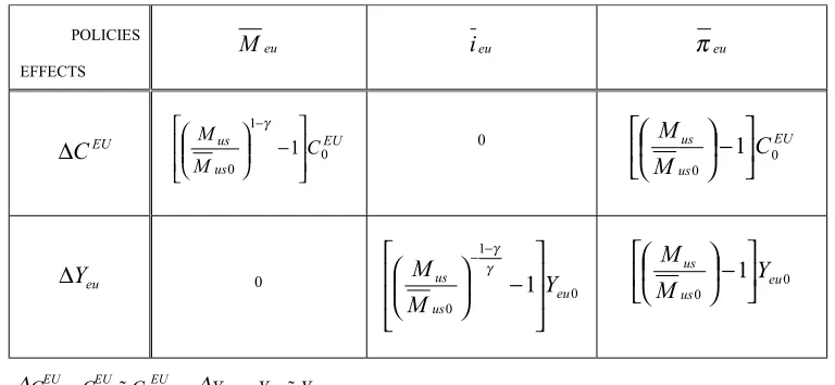
Table 1 summarizes the impact on European consumption and European output of a shock in the US money supply, under the alternative policy scenarios. Since the utility of consumers depends on consumption and leisure (which is a function of output), these effects will be important in determining the trade-offs between one rule and another. As seen before, when the stock of euro money balances is kept constant, output suffers no changes but European consumption is affected by the shock. On the other hand, if the nominal interest rate is kept fixed, Eurozone consumption remains stable but output adjusts. Under inflation targeting, both consumption and output will respond to the US monetary shock, given the change in the European money supply needed to maintain the inflation target. Under this policy regime, the proportional increase in consumption is exactly equal to the proportional increase in output. Given these results, it is clear that the relative impact of each of these policies on the utility of consumers will depend on the relative weight of consumption and output in the utility function.
22In the long run, the nominal exchange rate must respond to short-run and long-run changes in
the US money supply as follows:
EEU EEU =
µ
Mus Mus0
Mus Mus
¶−1
If the US monetary shock is reversed such that Mus = Mus0, the nominal exchange rate E
EU
will remain at the initial steady state level. However, if the increase in the US money supply is
permanent, thenMus=Musand the long-run nominal exchange rate will have to adjust by Mus Mus0
.
Table 1: Effects of a US money supply shock in Europe under alternative policy rules.
POLICIES
EFFECTS
eu
M ieu πeu
∆CEU EU
us us C M M 0 1 0 1 −
−γ 0 EU
us us C M M 0 0 1 − eu Y ∆ 0 0 1 0 1 eu us us Y M M −
−−γ γ 0 0 1 eu us us Y M M −
∆CEU = CEU ñ C0EU ; ∆Yeu = Yeu ñ Yeu0
4
Policies for the ECB
The ranking of alternative policies available to the ECB will be based on each policy’s ability to minimize the impact of exogenous shocks relative to the steady-state utility level. Formally the problem is to minimize the quadratic loss function:24
Leu =E[(U−U0)2]
Since utility depends on both consumption and output, policies should take into account of changes in both these variables. Although targeting the money supply mitigates the effects of a foreign monetary shock on output, such a policy cannot stabilize consumption - which depends on the world money supply - fully. Conversely, a fixed nominal interest rate policy is successful at insulating consumption from the monetary policy shock, but not as a buffer to output changes. Hence the use of one of these policy rules in isolation cannot fully insulate welfare from an external foreign policy shock.
24This chapter shows that the policy which maximizes utility given a positive shock will be the one
In Poole’s model (Poole, 1970), one policy was more successful than the other in stabilizing the economy depending on whether the shocks hitting the economy came from the expenditure sector, or from the monetary sector. To control for both types of shocks simultaneously, it was suggested that the monetary authority should pursue a combination policy, of a money and an interest rate target, in such a way that the weights take into account of the relative variance of the shocks. A similar trade-off between stabilizing the different components of utility (consumption and leisure) exits here, which can be addressed by a combination policy in a similar way to Poole’s suggestion. In order to analyze this formally, it is convenient to rewrite the loss function, such that:
Leu =β2E
"µ¡
C0EU¢1−ρln
µ
Mw Mw0

−K(Yeu0) 2
ln
µ
Meu Meu0
¶¶2#
(32)
using x'ln(x+ 1).25 Under a fixed monetary growth policy the loss function takes
the following form:
LM|eu =β2(1−γ)2
¡
C0EU¢2(1−ρ)σ2Mus (33) where σ2Mus is the expected variance of the US monetary shock .Alternatively, if the
ECB pursues afixed nominal interest rate rule, the loss function will be given by:
Li|eu =β2(1−γ)2
µ
1
γK(Yeu0)
2
¶2
σ2Mus
The two expressions can then be conveniently compared, by dividing one by the other. In addition define ξeu ≡
³
(CEU0 )(1−ρ)
´
/¡k(Yeu0)2
¢
, which can be understood as the relative weight of consumption versus output in the steady state utility function, to obtain:
LM
Li |eu= (γξeu)
2
(34)
where
ξeu = (C
EU
0 )(1−ρ)
k(Yeu0)2
= φ
(φ−1) 1
β(geu0)
Notice that ξeu is always positive.26 Since ξeu and γ are positive, the ratio (34) is
higher (lower) than one depending on whetherξeu is higher (lower) than the inverse of γ. Recall thatγ represents the effective macroeconomic size of the European economy,
25The algebra needed to derive the results in this section is shown in Appendix A.4.
26The relative weight of consumption and output in the utility function, ξ
eu, will be higher, the
in terms of the weight of the European goods in the world consumption, therefore, the inverse ofγ is proportional to the size of the US.
ξeu <
1
γ ⇒LM|eu < Li|eu ξeu > 1
γ ⇒Li|eu < LM|eu
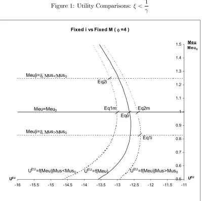
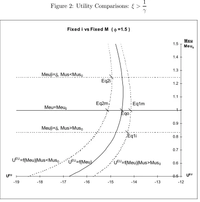
Afixed interest rate policy seems, therefore, to be more attractive for the European economy if the representative consumer attaches a higher weight on the utility derived from consumption rather than on the disutility from work. Conversely if the repre-sentative consumer attaches a larger weight on the disutility from work, it should be more prone to support a fixed money growth target. To illustrate graphically the choice between the nominal interest rate and the money growth rate for monetary policy targets two examples have been estimated, settingg0 = 1/0.9,β = 0.9, ρ= 4,
assumptions on the remaining parameters (low market power of workers), so that
[image:20.612.105.504.173.569.2]ξ <(1/γ).Figure 2 shows the case in which φ is low enough, given the values chosen for the other parameters (high market power of workers), such that ξ >(1/γ). Here the actual utility function is plotted, rather than the loglinear approximation.
Figure 1: Utility Comparisons: ξ < 1 γ
Fixed i vs Fixed M ( φ=4 )
0.5 0.6 0.7 0.8 0.9 1 1.1 1.2 1.3 1.4 1.5
-16 -15.5 -15 -14.5 -14 -13.5 -13 -12.5 -12 -11.5 -11
UEU
Meu
Meu0
Eqo
Eq2m Eq1m
Eq1i Eq2i
Meu|i=δ, Μus<Μus0
Meu|i=δ, Μus>Μus0
Meu=Meu0
UEU=f(Meu)
UEU=f(Meu)|Mus<Mus 0
UEU UEU=f(Meu)|Mus>Mus
Figure 2: Utility Comparisons: ξ > 1 γ
Fixed i vs Fixed M ( φ=1.5 )
0.5 0.6 0.7 0.8 0.9 1 1.1 1.2 1.3 1.4 1.5
-19 -18 -17 -16 -15 -14 -13 -12
UEU
Meu
Meu0
Eq2m
Eqo Eq1m
Eq1i Eq2i
Meu|i=δ, Mus>Mus0
Meu=Meu0
UEU=f(Meu)
UEU=f(Meu)|Mus<Mus 0
Meu|i=δ, Mus<Mus0
UEU UEU=f(Meu)|Mus>Mus
0
In both figures, the initial equilibrium point is denoted ‘Eqo’. The alternative
final equilibrium points, depending on whether the US follows an expansionary or a contractionary monetary policy, given that Europe follows a constant money supply rule, are labeled ‘Eq1m’ and ‘Eq2m’, respectively. In Figure 1, these are closer, in utility terms, to ‘Eqo’ than ‘Eq1i’ and ‘Eq2i’, which are the corresponding final equilibrium points when Europe follows a constant interest rate rule. In the case represented in Figure 1, where ξ < (1/γ), the fixed money supply rule stabilizes utility more. In Figure 2, when ξ > (1/γ), the opposite occurs: utility varies less when Europe follows a constant nominal interest rate rule.
com-pletely the economy from foreign shocks using either instrument alone. This is because with one instrument you can only pursue one objective, while stabilizing the utility function entails two. However, a combination policy, of the family proposed by Poole, in which the money stock and the nominal interest rate are maintained in a certain relationship to each other can solve the problem. In this case, the optimal relationship will have to take into account of the relative weight of consumption and output in the utility function and the relative size of the countries. Formally, such a combination policy can be defined as a relationship of the type:
µ
Meu Meu0
¶α
=
µ
1 +i
1 +δ
¶1−α
which minimizes the loss function, and where α determines the relationship main-tained between the money growth and the nominal interest rate target. The com-bination policy becomes a pure money growth rate policy, when α = 1, or a pure interest rate policy when α = 0. The value of the parameter α for which the loss function is zero for any value of σ2
Mus, determines the monetary policy rule which
insulates the economy from the US monetary shock. In this case that value is given by:27
α= (ρ−1)
(ρ−1)−ξeu; ξeu 6=
1
γ
whereξeu, is defined as before in (34).
The inability to stabilize welfare with only one instrument can also emerge under inflation targeting. In this model, under inflation targeting, the foreign monetary disturbance affects equally consumption and output. Hence this policy will only stabilize utility fully if the weights of consumption and output/leisure in the utility function are the same. Otherwise, a combination policy including inflation and either the money stock growth or the nominal interest rate can do better. Below these two types of policies will be denotedtwo-pillar policy with the nominal interest rate and
two-pillar policy with the money growth rate.
Formally, thetwo-pillar policy with the nominal interest rate, combining an infl a-tion and a nominal interest rate target, can be described by the following relaa-tionship:
µ
PEU PEU
0
¶απi
=
µ
1 +ieu
1 +δ
¶1−απi
which must minimize the loss function, and where απi determines the nature of the relationship between the variables in the combination. Whenαπi = 1the combination policy is a pure inflation targeting policy. Conversely, when απi = 0, it becomes a
purefixed interest rate rule. Under this rule, the value ofαπi which allows to insulate the economy from the US monetary disturbance is given by:28
απi = ρ−1
ρ−ξeu
; ξeu 6=
1
γ
If, on the other hand, the ECB decides to rely targeting the money stock, instead of the nominal interest rate, it will follow thetwo-pillar policy with the money growth rate. This strategy can be defined as a relationship between inflation and the money growth rate of the form:
Ã
PEU PEU0
!απM
=
µ
Meu Meu0
¶1−απM
which minimizes the loss function, and where απM determines the nature of the relationship between the two variables. This policy becomes a pure inflation target when απM = 1, and a pure constant money supply policy when απM = 0. In this case, the value of απM which sets the loss function equal to zero can be written as:29
απM = ξeu 2ξeu−1
; ξeu 6= 1
γ
In all cases the optimal combination policy is superior compared with the single or "pure" policy rules.30 It seems difficult to give preference for one kind of policy index
over the other, since they all facilitate insulation of the economy from the US money stock disturbance. However, the simpler the rule, the easier it will be to implement it properly. As in Poole (1970), the success of the combination policy depends on knowledge of the parameters and even the sign of the optimal relationship cannot be determined without such a knowledge: a combination policy based on intuition can be worse than either of the pure policy rules. Within this framework, the fact that
the two-pillar policy with the money growth rate (which combines the money stock
and inflation) does not require knowledge of the parameter of risk aversion, seems to be an advantage. Nevertheless, all combination policies require the knowledge of the parameter of monopolistic competition. The parameterφ determines the kind of relationship to be maintained between the policy variables, for a given market size,
γ, a given coefficient of time preference and a given steady state fiscal intervention parameter,geu0.31
28The calculations are shown in Appendix A.5.
29See Appendix A.5.
30Except in the particular case where the relative weights of consumption and leisure in the utility
function are the same. In that case inflation targeting can also achieve full welfare stabilization, but only for very restrictive set of parameters.
31Notice that it is only the level of the parameter of monopolistic competition in Europe that
It is important to notice though that all the “combinations” discussed so far allow the US money supply shock to pass-through to inflation, by the same amount. The changes in prices in the short run and in the long run are given by equations (35) and (36) whatever the “combination” policy pursued, when the policy parameterαj is set according to the optimal welfare criteria discussed before, forξeu 6= 1/γ:
PEU PEU0 =
µ
Mus Mus0
¶(1−γ)(ξeu−1)
1−γξeu
(35)
PEU PEU =
µ
Mus Mus0
¶ 1−γ
1−γξeu (36)
The total change in the price level, resulting from the shock is therefore:
PEU PEU0 =
µ
Mus Mus0
¶(1−γ)ξeu
1−γξeu
The only policy that allows to insulate inflation from the foreign money supply shock, in this model, is simple inflation targeting.
5
Other Policy Alternatives and Shocks
5.1
Other Policy Alternatives
The exchange rate is an alternative tool for the conduct of monetary policy in an open economy. Although the ECB has already stated that it will not follow any specific policy with regard to the exchange rate, it will inevitably monitor developments in this variable and take these into account when formulating policy. In order to keep the exchange ratefixed, the European monetary authority must set the money supply according to the following reaction function:
E =E0 ⇒Meu =
Meu0
Mus0
Mus
E =E ⇒Meu = Meu MusMus
Assuming that the US monetary authority changes its money stock permanently, that is, assuming that µ∗ is equal to one, then setting µ equal to one is enough to ensure that the policy rule is observed in the long run.32 In the short run, the
32Recall that µ∗=Mus
effect of this policy on consumption and output is exactly the same as under inflation targeting. Since output prices arefixed in the short run, movements in the consumer price index are due tofluctuations in the exchange rate. However, if the US money shock is permanent, under this policy regime, prices will have tofinally adjust in the long-run, such that:
PEU PEU =
Mus Mus0
As in the inflation targeting framework, under a fixed exchange rate regime, the foreign monetary disturbances produce a proportional effect on consumption and output, but this policy can only fully stabilize utility if the weights of consumption and output/leisure in the utility function are the same. Alternatively, a combination policy which includes the nominal exchange rate, and either the money stock growth or the nominal interest rate, can do better.33 Both types of combinations have already
been introduced in the literature. A combination between the interest rate and the exchange rate, usually referred to as the Monetary Conditions Index (MCI) and already used in practice by the Bank of Canada, for instance, has been recently analyzed by Freeman (1994). Combinatorial rules specifying trade-offs of monetary growth against exchange rate deviations from a pre-specified path, which will be denotedInternational Money Index, have been defended by Artis and Currie (1981) because of their ability to control for losses in competitiveness. They show evidence which suggests that the pursuit of monetary targets has frequently been associated with substantial and persistent real appreciation (German and Switzerland between 1978 and 1979 and the UK in 1977 and 1979-80), which can be avoided by including the exchange rate in the targeting rule.
Targeting aMonetary Conditions Index can be defined as targeting the relation-ship of the type: µ
Eeu Eeu0
¶αM CI
=
µ
1 +ieu
1 +δ
¶1−αM CI
which minimizes the loss function, and where αM CI determines the weight of each variable in the combination. If αM CI = 1 the combination policy is a pure fixed
33The first application of the instrument problem developed by Poole (1970) to the choice of an
exchange rate policy, while if αM CI = 0 this reduces to a pure interest rate rule. In this case the value of αMCI which insulates the economy from the foreign money supply shock is equal to:34
αM CI = (1−γ)(ρ−1)
(1 + (1−γ)(ρ−1))−ξeu; ξeu 6=
1
γ
TheInternational Money Index (IMI) targeting, on the other hand, can be defined
as a relationship between the exchange rate and the money growth rate of the form:
µ
E E0
¶αIM I
=
µ
Meu Meu0
¶1−αIM I
which minimizes the loss function, and where αIM I determines the nature of the relationship between the two variables. The IM I policy collapses into a pure fixed exchange rate policy whenαIMI = 1and into a pure money supply rule whenαIM I = 0. The value of αIM I for which the loss function is minimized is now equal to:35
αIM I = (1−γ)ξeu
(2−γ)ξeu−1; ξeu 6= 1
γ
As in the case of the two-pillar policy with the money growth rate no knowledge of the parameter of risk aversionρis required to implement this policy rule. However a precise knowledge ofγ (the world market share) is required, in this case.
Other possible rules could also be analyzed. Nominal income targeting, for in-stance can be obtained as special case of targeting an index containing the nominal exchange rate and the money stock. This can be seen by writing the expression for the short-run nominal income growth as follows:
PEU PEU0
Yeu Yeu0
=
µ
E E0
¶1−γ Meu Meu0
The intuition behind this is that, in the short run, the price index responds to changes in the nominal exchange rate while real output responds to changes in the money stock. Nominal income targeting however, implies maintaining a particular relation-ship between the exchange rate and the money stock which is exactly given by the relative share of US goods in the world market, as shown in equation (37).
PEU PEU0
Yeu Yeu0
= 1⇒
µ
E E0
¶1−γ1
=
µ
Meu Meu0
¶1
γ
(37)
34The calculations are shown in Appendix A.5.
This relationship will only correspond to the optimal IM I described in section 5, if the relative weight between consumption and output in the utility function is equal to1/2, that is, the output term in the steady state utility function has to have twice as much weight as the consumption term for a nominal income strategy to be able to fully stabilize utility. Recall that the optimal relationship between the exchange rate and the money shock, determining theIM I implies:
αIM I = (1−γ)ξeu (2−γ)ξeu−1
Hence, targeting nominal income will only be equivalent to using the optimal IM I
targeting providedαIM I = 1−γ1, that is, as long as the following condition is satisfied:
(1−γ)ξeu
(2−γ)ξeu−1
= 1− 1
γ ⇒ξeu =
1 2
Although the discussion presented here has only focused on one type of distur-bance, namely US money shocks, these are in fact quite interesting for analyzing monetary policy rules. These shocks are an example of a foreign disturbances in re-sponse to which the policy maker has an interest to focus on variables that reflect external economic conditions (consumer price indexes, the interest rate and the ex-change rate). In addition because they are nominal shocks, they affect real variables only in the short run, which corresponds to the time horizon for which monetary pol-icy is effective. Nevertheless, the next subsection outlines the results for other types of shocks.
5.2
Other shocks
The analysis illustrates in the context of an open economy, in which “home” con-sumption may differ from production, the existence of a trade-off in terms of welfare stabilization through the use of different policy rules. This trade off can be better resolved with “combination” rules.
On the contrary, if temporary US fiscal shocks are taken into account, the best policy alternative is always to let the money stock remain constant since, in the short run, neither European consumption nor European output respond to the US
between long-run and short-run movements in the real variables.36 Fixing the money stock produces a larger overshooting/undershooting of output, in the case of "home"
fiscal shocks. However, under interest rate targeting there is a short-run change in consumption, that only occurs in the long-run under a money growth rule, that is, when the nominal interest rate is keptfixed changes in consumption are anticipated one period relative to the case where the money stock is kept fixed. Appendix A.6 summarizes these results. In what concerns shocks to the parameters of the model, only shocks to the coefficient of risk aversion (ρ) or the market share (γ) could matter in answering the questions raised in the context of this model, because the nominal interest rate does not react to changes in the parameters of monopolistic competition in the labor market; but no parameter changes were analyzed here.
6
Conclusions
The purpose of this paper is to evaluate whether a monetary policy strategy con-sisting of multiple intermediate targets (such as money growth and inflation) can be superior to an adoption of a single target, such as inflation targeting. Three diff er-ent policies — money growth targeting, interest rate targeting and inflation targeting — were compared in terms of their effectiveness in mitigating a foreign-induced (i.e., US) monetary shock. These alternative policies were ranked according to their ability to stabilize inflation and, alternatively, the utility of consumers. It was shown that, when the utility of consumers depends on both consumption and leisure, rather than targeting a single intermediate target, the central bank can achieve a better outcome, in terms of welfare stabilization, by combining two different intermediate targets. In terms of inflation stabilization, the paper confirmed that inflation targeting does achieve the best outcome, while combining inflation with the interest rate, or money growth, or combining money growth with the interest rate all yield somewhat higher inflation variability. Nonetheless, any of these combination policies, while sacrificing some price stability, may in fact achieve a better outcome in terms of full welfare stabilization. In order to achieve this outcome, policymakers need to know the un-derlying parameters of the model (e.g., the degree of risk aversion, the market power of workers, the intertemporal discount rate, etc.).
However, when uncertainty regarding these parameters is high, a poorly designed “combination” policy can exacerbate the effect of shocks on consumption and output. Interestingly, a policy combining the inflation rate and the money growth rate does
36Temporary home fiscal shocks are uninteresting because the nominal interest rate does not
References
[1] Artis, M. and Currie, D. (1981) “Monetary Targets and the Exchange Rate: A Case for Conditional Targets”, in Eltis, W. and Sinclair, P. (1981) The Money
Supply and the Exchange Rate, Clarendon Press, Oxford.
[2] Collard, F., Dellas, H. and Ertz, G. (2000), “Poole Revisited”, Centre for Eco-nomic Policy Research, disussion paper No.2521.
[3] Barro, R. and Gordon, D. (1983) “Rules, Discretion and Reputation in a Model of Monetary Policy”, Journal of Monetary Economics, 12 (1), 101-122.
[4] Blanchard, O. and Kiyotaki, N. (1987) “Monopolistic Competition and the Ef-fects of Aggregate Demand”, American Economic Review, 77 (4), 647-666.
[5] Boyer, R. (1978) “Optimal Foreign Exchange Market Intervention”, Journal of Political Economy, 86(6), 1046-1055.
[6] Calvo, G. (1983) “Staggered prices in a utility-maximizing framework”, Journal of Monetary Economics 12(3), 383-398.
[7] Cole, H. and Obstfeld, M. (1991) “Commodity Trade and International Risk Sharing: How Much do Financial Markets Matter?”, Journal of Monetary Eco-nomics 28 (1991), 3-24.
[8] Corsetti, G. and Presenti, P. (1999) “Welfare and Macroeconomic Interdepen-dence”, unpublished version (previous version published as NBER wp 6307, Dec 1997, next version forthcoming Quarterly Journal of Economics).
[9] Dixit, A. and Stiglitz, J (1977) “Monopolistic Competition and Optimal Product Diversity”, American Economic Review, 67, 297-308.
[10] Freeman, C. (1994) “The Use of Indicators and a Monetary Conditions Index in Canada” in Bank of Canada, Economic Behavior and Policy Choice under Price Stability, 1994.
[11] Ghironi F. (1998) “U.S.-European Economic Interdependence (I): Positive Analysis”, unpublished paper.
[12] Obstfeld, M. and Rogoff, K. (1996) Foundations of International Economics, Cambridge, MA, MIT Press.
[13] Obstfeld, M. and Rogoff, K. (1998) “Risk and Exchange Rates”, NBER, wp.6694
[15] Poole, W. (1970) “Optimal Choice of Monetary Policy Instruments in a Simple Stochastic Macro Model”, Quarterly Journal of Economics, 84, 197-216.
[16] Sargent (1987) Macroeconomic Theory, 2nd ed. Orlando, FL, Academic Press.
[17] Taylor, J. B. (1980) “Aggregate Dynamics and Staggered Contracts”, Journal of Political Economy, 88 (1), 1-23.
[18] Taylor, J. B. (1993) “Discretion versus policy rules in practice”, Canergie-Rocehester Conference Series on Public Policy, 39, 195-214.
[19] Woodford, M. (1991), “Currency Competition and the Transition to Monetary Union: Does Competition Between Currencies Lead to Price Level and Echange Rate Satbility?”, in Alberto Giovannini and Colin Mayer (eds),European
A
Appendix
A.1
Solving the problem of consumers
The wealth Ωτ−1, consisting of last period’s wage income, lump-sum transfers, cash
balances, and assets plus interest earnings that have not been spent on last period’s consumption, can be formally written as:
Ω(j)τ−1 ≡
¡
Weu(j)τ−1Leu(j)τ−1+PτEU−1Teuτ−1
¢
+¡MeuEU(j)τ−1+Eτ−1MusEU(j)τ−1
¢
+ +¡PτEU(1 +reuτ−1)AEUeu (j)τ−1+PτEU(1 +rusτ−1)AEUus (j)τ−1
¢
− −¡Peuτ−1CeuEU(j)τ−1+Eτ−1Pusτ−1CusEU(j)τ−1
¢
This section shows the conditions needed for deriving the solution of the model, for the case of Europe. The solution for the case of the US is analogous. Given that in the optimum the cash-in-advance constraints (4) and the budget constraint (5), will be binding, the Lagrangian for this problem can be simplified to the expression below:
$t =
∞
X
τ=0
βτ
·
CEU(j)1−ρ τ
1−ρ +V(Geuτ)− k
2Leu(j) 2
τ +λτ(Λeut)
¸
Λeut ≡ (Leu(j)
1−1φ
τ−1 Peuτ−1Yτ−1 1
φ +PEU
τ−1Teuτ−1) +
+¡PτEU(1 +reuτ−1)AEUeu (j)τ−1+PτEU(1 +rusτ−1)AEUus (j)τ−1
¢
− −¡PeuτCeuEU(j)τ +EτPusτCusEU(j)τ +PτEUAeu(j)τ +PτEUAus(j)τ
¢
which has the following ‘First Order Conditions’ (FOCs):
CEU(j)1t−ρ
γ PeutCEU
eu (j)t
=λt (38)
CEU(j)1t−ρ
1−γ EtPustCEU
us (j)t
=λt (39)
−λt+βλt+1(1 +reut) = 0 (40)
−λt+βλt+1(1 +rust) = 0 (41)
−kLeu(j)t+βλt+1
φ−1
φ Leu(j)
−1
φ
t PeutYeut
1
φ = 0 (42)
Using equations (38) and (39) it is then possible to write that:
γ
PeutCEU(j) =
Rearranging this relation yields the following relationships:
PtEUCtEU =PeutCeuEU(j)t+EtPustCusEU(j)t=
1
γPeutC EU eu (j)t=
1
1−γEtPustC EU us (j)t
(43) which can be used together with equation(38) to obtain:
λt=CEU(j)−tρ
Arbitrage in the asset market determines that reut =rust =rt, for all t. This follows from satisfying (40) and (41) simultaneously. Substituting λt = CEU(j)−ρ
t , for all t, into one of these last equations and into (42) yields, respectively, the usual Euler equation and a labor-leisure trade-off:
µ
CEU(j) t+1
CEU(j) t
¶ρ
=β(1 +rt)
Leu(j)t=β φ−1
kφ Leu(j)
−φ1
t Yeut
1
φ Peut PEU
t
PtEU PEU t+1
CEU(j)−t+1ρ = 0
Assuming symmetry the indexj can drop out andLeu(j)t =Leut=Yeut. In this case
the conditions for optimality become:
µ
CtEU+1
CEU t
¶ρ
=β(1 +rt) (44)
Yeut =βΦPeut
PEU t
PEU t PEU
t+1
¡
CtEU+1
¢−ρ
(45)
whereΦ= φ−1
kφ . Finally the transversality condition for this problem, which ensures
that no wealth is accumulated at timet+τ, whenτ tends to infinity, is given below.
lim
τ→∞
1
t+τ
Y
s=t+1
(1 +rs)
µ
AEUeut+τ +AEUust+τ +M
EU
eut+τ +Et+τMustEU+τ PEU
t+τ

= 0
A problem, in all respects analogous to this, is solved by US consumers.
A.2
Model Solutions
implies that the interest rate in real terms is equalized across the Atlantic, it follows that the following relation between European and US consumption changes must hold.
CEU CEU =
CU S
CU S (46)
where, as indicated earlier, variables with a bar on top describe the long run and variables without a bar describe the short run. This condition, rearranged, shows that the international consumption ratios are the same in the long and in the short run. In addition, another link between the short run and the long run can be found in the current accounts for thefirst period of the new steady state:
N F AEU = (1 +reu)N F AEU +Peu(Yeu−Geu)
PEU −
CEU (47)
N F AU S = −(1 +rus)N F AU S+Pus(Yus−Gus)
PUS −C U S
(48)
where, assuming that the initial stock of external debt is zero, that is, N F AEU
0 =
N F AEU0 = 0, the consumption indexes in the short run must satisfy:
CEU = Peu(Yeu−Geu)
PEU −N F A EU
CU S = Pus(Yus−Gus)
PUS −N F A U S(49)
CEU = δN F AEU+Peu(Yeu−Geu)
PEU C U S
=δN F AU S+Pus(Yus−Gus)
PU S (50)
SubstitutingCEU derived from equation (50) into equation (47) it can be shown that
(1 +δ)N F AEU = (1 +reu)N F AEU. Substituting Peu(Yeu
−Geu), Pus(Yus −Gus),
Peu(Yeu −Geu) and Pus(Yus −Gus) using the market clearing conditions (8), into
equations (49) and (50) and dividing the European by the US current account, yields the following equilibrium relations:
CEU+N F AEU CU S+N F AU S =
γ
1−γ
CEU−δN F AEU CUS −δN F AU S =
γ
1−γ (51)
Recall that N F AU S
t = −N F AEUt , for all t. Given that (1 + δ)N F A EU
= (1 +
reu)N F AEU, equations (51), together with equations (46) imply that N F AEU = N F AEU = 0 andN F AU S = N F AU S = 0. Substituting these results into equations
(51) gives the ratios of European to US consumption, in the long run and in the short run, which are always constant and equal toγ/(1−γ).
CEU CUS =
CEU CU S
= γ
In the case of the model presented here, relaxing the assumption that the initial external debt is zero could allow temporary shocks, with an impact in the real interest rate, to induce current account changes, but for simplicity this alternative was not pursued.37
To help solve the model, it is simpler to define the following indexes offiscal stance:
geu ≡ Yeu/(Yeu −Geu) and gus ≡ Yus/(Yus −Gus). Notice that geu (gus) is equal to one whenGeu (Gus) is zero and is increasing inGeu/Yeu(Gus/Yus). In addition define also the following world aggregates (xwt) and the following relative indexes (xRt):
xwt≡(xeut)γ(xust)1−γ xRt ≡xeut/xust (53) wherexeu can be any of Europe’s variables. Given a variablexeu,xusstands for its US analogue. Notice thatxeut= (xRt)1−γxwtandxust = (xRt)−γxwt. In what concerns the
parameters of the model, for any parametersα (referring to the European economy) andα∗ (referring to the US economy), similar aggregates will be defined whenever it is convenient, such that: αw ≡(α)γ(α∗)1−γ andαRt
≡α/α∗.
Now it is possible to solve for the long-run equilibrium in this model. First recall the goods market clearing conditions (8). In the long run these conditions become:
Peu(Yeu−Geu) PEU
=γ(CEU +CU S)
Pus(Yus−Gus) PUS
= (1−γ)(CEU +CU S)
SubstitutingCU S = 1−γ
γ C EU
in the European goods market equilibrium andCEU =
γ
1−γC U S
in the US goods market equilibrium and substituting (Yeu − Geu) by Yeu/geu and (Yus −Gus) by Yus/gus, according to the notation introduced before,
yields:
PeuYeu PEUgeu =C
EU PusYus PU Sgus =C
U S
(54)
Replacing these results in the long-run versions of the quality-theory-of-money equa-tions (10), gives the equilibrium locusM C, providing a relationship between the real stock of money and consumption:
M C : Meu
PEU
= Peu
PEU Yeu
geu
⇒ Meu
PEU
=CEU (55)