Fingerprint recognition through circular sampling

(1)

Rochester Institute of Technology

RIT Scholar Works

Theses Thesis/Dissertation Collections

1999

Fingerprint recognition through circular sampling

David Chang

Follow this and additional works at:http://scholarworks.rit.edu/theses

This Thesis is brought to you for free and open access by the Thesis/Dissertation Collections at RIT Scholar Works. It has been accepted for inclusion in Theses by an authorized administrator of RIT Scholar Works. For more information, please [email protected].

Recommended Citation

(2)

SIMG-503 Senior Research

Fingerprint Recognition Through Circular Sampling

Final Report

David H. Chang Center for Imaging Science Rochester Institute of Technology

May 1999

(3)

Table of Contents http://www.cis.rit.edu/research/thesis/bs/1999/chang/contents.html

Fingerprint Recognition Through Circular Sampling

David H. Chang

Fingerprint Recognition Through Circular Sampling

David H. Chang

Abstract

The uniqueness of the human fingerprint is considered to be one of the most reliable characteristics for personal identification. Considering that we leave them on nearly all of the surfaces we touch, they become valuable to those in law enforcement for identifying perpetrators of a crime. However, the matching of a single fingerprint with the millions that have been catalogued proves to be a difficult task. This study presents an alternate method to fingerprint recognition by way of a spatial re-sampling of the pattern through concentric circles. With this approach, the

concentric circular samples have rotation invariant features while a translation is dependent only on the location of the circles' center. The resulting circles are then correlated with those from the known set to obtain a collection of the most probable matches. This technique has shown exceptional results when comparing various binary test patterns as well as synthetic binary fingerprint images but is unable to recognize unenhanced greyscale fingerprint images.

(6)

Copyright © 1999 Center for Imaging Science

Rochester Institute of Technology

Rochester, NY 14623-5604

This work is copyrighted and may not be reproduced in whole or part without permission of the Center for Imaging Science at the Rochester Institute of Technology.

This report is accepted in partial fulfillment of the requirements of the course SIMG-503 Senior Research. Title: Fingerprint Recognition Through Circular Sampling

Author: David H. Chang Project Advisor: Joseph P. Hornak SIMG 503 Instructor: Joseph P. Hornak

(7)

Acknowledgement http://www.cis.rit.edu/research/thesis/bs/1999/chang/acknowledgement.html

Fingerprint Recognition Through Circular Sampling

David H. Chang

Acknowledgement

Well, first off I need thank my mom and dad for their love and support over my four years at RIT. They have pushed me to work hard without much nagging and have instilled in me their trust all the while without asking anything about the many empty liquor bottles in my apartment. Of course they all belonged to my roommates. ;-)

Next I must give gratitude to those responsible for giving out the Perkins loans and Direct loans but more importantly, I want to thank RIT for their scholarships, the state of New York for the TAP grant, and the US government for the federal Pell grant. See, not everyone despises big brother!

Now I wish to recognize all of my CIS friends but particularly Monica, an amazingly charming and sincere woman who with the ever witty and venerate Lana forms the awesome dynamic duo known as LANICA!, the wonderfully audacious and sweet Janel along with "Sunshine" Dave, and last but certainly not least, that beautiful Greek we all know as Pano. Thank you all for being my friends.

Finally, I want to praise the undisputedly great members of the CIS staff especially Dr. Joseph P. Hornak for his help, advise, patience, and that cool bloody fingerprint on glass picture.

(8)

Fingerprint Recognition Through Circular Sampling

David H. Chang

1 Introduction

The use of one’s fingerprints as a means of identification has existed long before its common usage today in the field of criminal investigation. Prior to the nineteenth century, fingerprints were primarily used only as a signature for indicating authorship or ownership. Other applications were not acknowledged until about 1860 when

William Hershel was regularly imprinting the handprints of those engaged in his contracts. It was not until 1881 when Henry Faulds recognized that fingerprints found at crime scenes may be used to identify the perpetrator. Further exploration into fingerprints followed when Sir Francis Galton began his research in the field and authored the first textbook on fingerprinting in 1892. As a result of the work of these individuals, fingerprinting was soon

accepted by Scotland Yard and finally by the United States in 19101.

Today, fingerprints are perhaps the primary means of personal identification although there are many other unique characteristics of an individual that can be used. They include voiceprints, dental impressions, DNA, retinal

patterns, and even the shape of the ear lobes1. Although these other characteristics are as much unique to the individual as are fingerprints, they lack many advantages which fingerprints have especially for the criminal investigator and forensic scientist. Common to the other distinctive attributes, fingerprints are universal and unique. In other words, everyone has them and no two have ever be en found to be identical. Fingerprints are also unchangeable. They are formed before birth and remain until decomposition of the skin occurs some time after death. Although some deformities may result from aging, manual labor, or scarring, the overall pattern always remains distinguishable. What make fingerprints preferable are that they can be easily attained, quickly classified, and are very likely to be found at crime scenes. Not only can they identify criminals but also casualties of

disasters such as plane crashes. Another common application is in maintaining access control.

Since 1924, the FBI has accumulated about 30 million sets of fingerprints2 making the matching of a single fingerprint with such a collection very difficult. With the advent of advanced computer technology in the past few decades, automated fingerprint identification systems (AFIS) can effectively perform what would otherwise be a laborious and time consuming task. This study presents a method to fingerprint recognition by way of a spatial re-sampling of the pattern through concentric circles. With this approach, the concentric circular samples have rotation invariant features while a translation is dependent only on the location of the circles' center. The resulting circles are then correlated with those from a known set to obtain a collection of the most probable matches.

2 Background

2.1 Fingerprint Uniqueness

What actually makes a fingerprint unique depends on one main factor. Fingerprints basically consist of ridges (raised skin) and furrows (lowered skin) that twist to form a distinct pattern. When an inked imprint of a finger is made, the impression created is of the ridges while the furrows are the uninked areas between the ridges.

Although the manner in which the ridges flow is distinctive, other characteristics of the fingerprint called ‘minutiae’ are what is most unique to the individual (See figure 1 for several minutiae representations). These features are particular patterns consisting of terminations or bifurcations of the ridges. It is these features that

(9)

[image:9.612.181.434.29.164.2]

Fingerprint Recognition Through Circular Sampling http://www.cis.rit.edu/research/thesis/bs/1999/chang/thesis.html#1

Figure 1. Minutiae examples

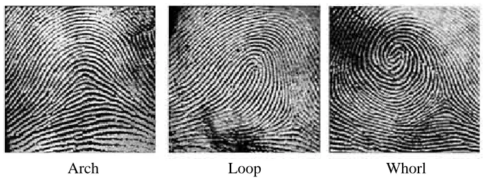
Moreover, all fingerprints can be classified into three categories based on their major central pattern4. These patterns are the arch, loop, and whorl, which are shown in figure 2. The importance of these three patterns will be described in more detail in the methods section.

Figure 2. Three major fingerprint classifiers

Arch Loop Whorl

2.2 Matching Difficulties

Several obstacles exist that make the matching of fingerprints a difficult task. The major obstacles are rotation, displacement, missing areas, and image defects. Rotation and displacement effects as well as image defects are problematic as variations occur each time fingerprints are taken and digitized. Aligning the finger for impression in the same registration and orientation every time would be impossible while improper inking along with the noise of the scanning system commonly attribute to image defects. THese factors are even more difficult to control considering that the fingerprints under question are typically latent prints found at a crime scene. These are prints left unintentionally on some surface that is not necessarily paper and impressioned in something that is not likely to be ink. It is expected that these prints are poor in quality and often have many missing or indisernible areas. The fingerprint identification system must account for each of these factors. Other factors exist as well but will not be investigated in this research. For instance, the scaling of the fingerprint is often considered as someone may be identified even though their fingerprints were recorded at a very young age.

2.3 AFIS Recognition Process

Digitized fingerprint images are obtained either through a dedicated fingerprint scanner or the standard scanning of inked fingerprint impressions. The prints are scanned at a resolution of 500 dpi with 8 bits per pixel with digital images having dimensions of 512 x 512 pixels (approximately 1" x 1") and 256 gray levels. This is the

criterion as recommended by the FBI5

and is employed in this research. Once the images have been acquired, they are put through an image enhancement procedure to remove unwanted image defects and modify properties for certain purposes.

[image:9.612.129.481.259.392.2]

(10)

3 Theory

3.1 Sampling and Concentric Circular Sampling

An image, such as that of a fingerprint, may be considered as a two-dimensional continuous signal. By this, it can have an infinite number of brightness intensities in an infinitesimal area. In order for an image to be handled by a computer, it must first be digitized.

Digitizing removes the continuous condition of the image through sampling and quantization thereby making the signal discrete. By sampling, the image is spatially approximated by repeatedly recording the averaged intensity within a region at regular intervals throughout the entire area. With quantization, the intensities are approximated to finite levels. These values, often termed gray levels, are then stored into a two-dimensional array where each cell in the array maps to a corresponding sample point. These cells are commonly called picture elements or pixels. Because the information between the sampling intervals in the image is lost, it is often desired that the interval size be controlled. This is achieved by managing the number of sampling points to be used over a certain distance. This is referred to as resolution. Likewise, the number of gray levels may also be regulated.

For this study, the image had to be sampled in a different manner. Instead of sampling in the general Cartesian space, the image is sampled through a pattern consisting of concentric circles. It may be considered that this technique is sampling in a polar coordinate space. Under this approach, the sampling resolutions are the distance between the concentric circles and the sampling interval within the circumference of the circles.

Figure 3. Sampling procedures

Image

Sampled Signal

However, there are currently no available digitizing devices that can sample images in such a fashion. Devices such as scanners and digital cameras, sample in a raster fashion. To overcome this obstacle, an algorithm can be developed to perform concentric circular sampling on the data obtained through conventional sampling. This

achieved with the Bresenham's circle generation algorithm8. The algorithm computes the coordinates that best approximates a circle for a given radius with the center having the coordinates (0,0). For concentric circles, additional circle coordinates are computed with radius values being a incrementing multiple of a given Δr. To resample an image, a registration point is required for the location of circles' center. The values at the pixel locations given by the sum of the circle coordinates and registration point are then recorded. In the subsequent sections, the array of values will often be referred to as f_pn(i) where p is a reference to the image that was sampled, n is the circle number, and i is the index of a particular sample point. In addition, I will represent the total number of sampling points for a particular circle and N will be the total number of concentric circles.

3.2 Correlation

(11)

area of the product of the two signals.

(1)

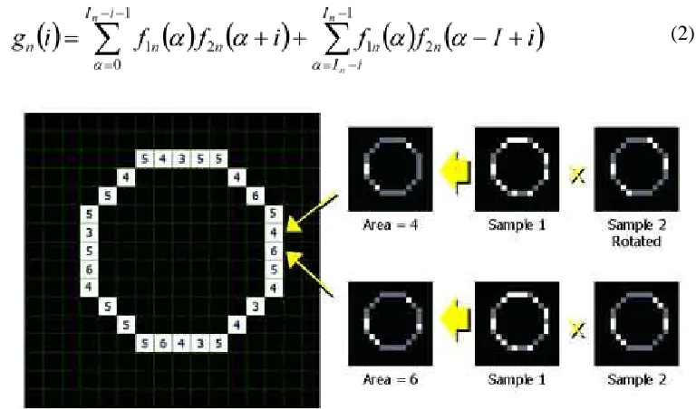
Equation 1 however, is expressed for continuous signals when it must be applied to discrete signals for this study. In addition, the correlation operation is performed in a circular fashion so that the shifted signal must wrap around the other. This procedure is shown in Figure 4 with its equation given by Equation 2.

[image:11.612.112.496.165.391.2]

(2)

Figure 4. Circular correlation process

4 Methods

The following procedures were performed through routines provided in the appendix.

4.1 Test Images

Prior to testing the present matching process on fingerprint images, a series of test images were created to observe for any perculiarities in the algorithms. These images consisted of fragments of lines varying in frequency, orientation, and thickness.

4.2 Synthetic Fingerprint Images

Another set of test images were of synthetic fingerprint images created through a demo software called Fingerprint Creator by Optel http://www.OPTEL.com.pl/index_en.htm. With the various minutiae types randomly placed in each generated image, these images are useful in showing well how the present matching algorithm performs. However, these artificial images are not realistic enough that it can be assumed the same results will occur for actual fingerprints.

All test images were 512 x 512 pixels in size with one bit per pixel.

4.3 Match Metrics

(12)

samplings of two fingerprint images being compared. The three metrics are the area ratio, correlation fraction, and angular density. The metrics are actually performed on each individual circle pair and and averaged over all the circles. A value of one indicates a perfect match while a zero would indicate a very poor match.

4.3.1 Area Ratio

One way of considering two signals as being similar is through their areas. This metric, given by Equation 3, only measures the ratio the smaller area to the higher area between the two circular signals being compared. A perfect match occurs if the two signals have equal areas.

(3)

Where A_pn is the area of the nth circle signal in image p as given by equation 4.

(4)

Where f_pn(i) is the nth circle signal of image p having I number of samples.

4.3.2 Correlation Fraction

As mentioned in section 3.2, the location of the highest magnitude in the correlation of two signals indicates where the two signals were most similar. Since in this research the signals are binary, meaning they can only have values of zero or one, the product of the two signals being compared may be considered as a signal containing their common area. With this in mind, it can be stated that the correlation between two binary signals can not have a magnitude greater than the smaller area of those signals. Based on this knowledge is the correlation fraction metric, which is given by Equation 5.

(5)

Where V is the notation for the maximum operation.

4.3.3 Angular Density

The angular density metric measures the match likelihood by determining how closely the locations of the highest match in each circle corresponds to that in the other circles of the correlation signal. This is achieved by the following steps.

(13)

(6)

The set of angles are then converted to a set of unit vectors whose coordinates are given by equation 7.

(7)

The vector components are averaged as given by equation 8.

(8)

The mean square error (MSE) is then calculated for the x and y vectors through equation 9.

(9)

The angular based MSE is then calculated from the vector based MSE through equation 10.

(10)

Finally the angular density metric is defined by equation 11.

(11)

4.4. Matching Process

(14)

Figure 5. Fingerprint with missing area

5 Results

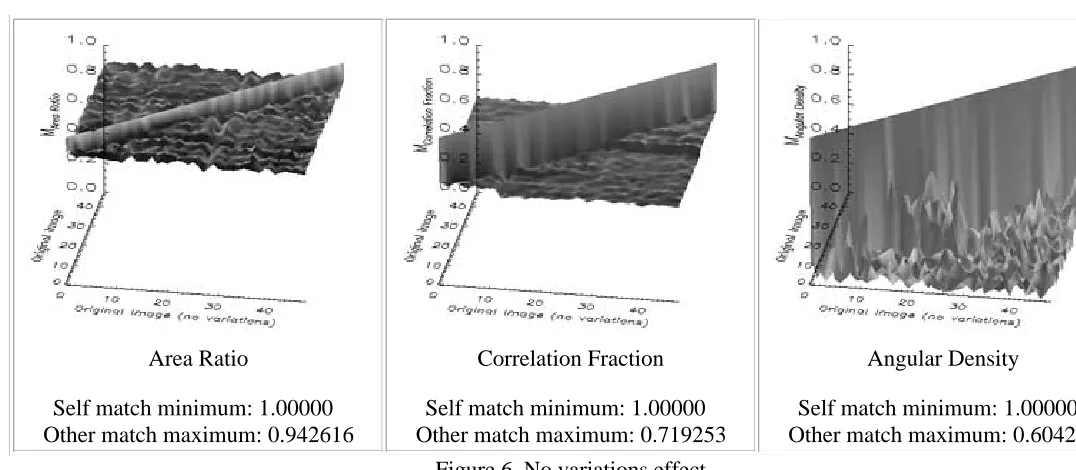
The following surface plots are the 48x48 match matrices. Along the x-axis (lower horizontal axis) are the fingerprint images dependent on some variation matched against the original unvaried images along the y-axis (side axis) while the value of the match metric in question is plotted along the z-axis (vertical axis). Also given for each matrice are the self match maximim and other match minimum values. The self match minimum is the smallest metric value determined along the diagonal where the varied image is match against itself. The other match maximum is the largest metric value determined at all locations not including the diagonal where the varied image is match against other images in the set (does not include itself). Ideally, the self match minimum should have a value of 1.0 while the other match maximum a value of 0.0. This however would not occur so it can only be desired that the self match minimum value be close to 1.0 and be greater than the other match maximum. If this holds true, a threshold may then be set between these values so that unknown images may be tested against this database.

[image:14.612.37.575.293.528.2]

5.1 Observation of Peculiarities Without Variations

Figure 6. No variations effect Area Ratio

Self match minimum: 1.00000 Other match maximum: 0.942616

Correlation Fraction

Angular Density

(15)

[image:15.612.42.577.24.248.2]

Figure 7. Missing area effect Area Ratio

Angular Density

[image:15.612.40.576.287.538.2]

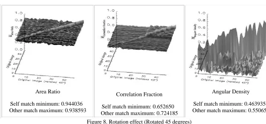
5.3 Observation of Rotational Effect

Figure 8. Rotation effect (Rotated 45 degrees) Area Ratio

Angular Density

5.4 Observation of Displacement Effect

(16)

Figure 9. Displacement effect

6 Discussion

6.1 Peculiarities Without Variations

With this procedure, it was determined that all the metrics were able to successfully determine the correct match. However, the angular density metric proved to show the best match given that its other match maximum of 0.604292 was lower than 0.942616 and 0.719253 found in the area ra tio and correlation fraction metric respectively.

6.2 Missing Area Effect

With this experiment, we can expect that the area ratio metric fails since it is dependent only on the area of the signals. With the Correlation fraction metric, there was actually improvement with the signal having been manipulated in this manner. However, this occurrence can be explained by the behavior of the correlation operator. If one of the two signals has more locations with no magnitude, there is a greater chance for that signal with the lesser magnitude to be matched against the other. Since this metric does not consider the locations of highest correlation, it is not as reliable as the angular density metric though it shows better results. This is not to say that the angular density metric fails, which it does not. It still shows a self match minimum of 0.620960 that is fortunately a good amount greater than the other match maximum of 0.489653.

6.3 Rotational Effect

(17)

6.4 Displacement Effect

As can be seen from Figure 9, a shift no more than a single pixel in any direction is permissible in the case of the area ratio and correlation fraction metric. The angular density metric however, allows for a little greater flexibility as it would still indicate a match if the center is displaced beyond the specific location by up to three pixels in any direction. This is particularly true in the case of a whorl type fingerprint but less so in the other two.

7 Conclusions

Given the results as discussed earlier, it is evident that the fingerprint images can be successfully matched through the proposed concentric circular sampling technique by way of the angular density metric. This metric performs very well for recognizing fingerprints that have missing areas. The results from the effects of rotation are acceptable while displacement effects are least problematic for this metric when compared to the other metrics. Overall, this technique shows exceptional results for matching the synthetic binary fingerprint images and similar results are expected if tested on enhanced actual fingerprint images. Of course the enhancement of the actual fingerprints must include binarization since that is a requirement of this technique.

In consideration of matching speed, the approach of this study cannot accurately determine a match without comparing the fingerprint under question to the entire known set. This is necessary if the desired result of this matching process is a collection of the most probable fingerprints. For small fingerprint databases, this would not be a major dilemma but in consideration of the FBI's massive set, this would be unacceptable given the amount of time required. However, there are those that have a need for fingerprint identification given a small database. Such an example would be businesses having to maintain access control.

7.1 Future Work

The current research is somewhat of a preliminary study into the possibility of performing fingerprint recognition through the proposed alternative approach that is circular sampling. Some suggestions for further research into this approach are presented.

A more efficient approach would require a means of classification prior to matching. This would greatly reduce the number of matches that need to be performed thus improving the overall matching speed. Also beneficial to the matching speed would be optimized code since the number of computations could be reduced. Since this technique is directed at binary images, further study may include an application towards images other than fingerprints such as text characters.

(18)

Fingerprint Recognition Through Circular Sampling

David H. Chang

References

R. O. Arthur, "Fingered," pp. 116-139, in The Scientific Investigator, ed. by Charles C. Thomas, Springfield, 1965 1.

V. Wickerhauser, Adapted Wavelet Analysis from Theory to Software, AK Peters, Boston, 1994 2.

L. Hong, Y. Wan, and A. Jain, Fingerprint Image Enhancement: Algorithm and Performance Evaluation, IEEE Transactions on Pattern Analysis and Machine Intelligence 20, pp. 777-789, 1998

3.

H. C. Allison, Dactylography-Dermatoglyphics, pp. 121-135, Personal Identification, Holbrook Press, Inc., Boston, 1973

4.

D. C. D. Hung, "Enhancement and Feature Purification of Fingerprint Images," Pattern Recognition 26:1661-1671, (1993).

5.

S. Singh, 2D Spiral Pattern Recognition With Possibilistic Measures, Pattern Recognition Letters 19, pp. 141-147, 1998

6.

K. V. Mardia, A. J. Baczkowski, X. Feng, and T. J. Hainsworth, Statistical Methods for Automatic Interpretation of Digitally Scanned Finger prints, Pattern Recognition Letters 18, pp. 1197-1203, 1997

7.

D. F. Rogers, Procedural Elements for Computer Graphics 2nd ed., pp. 79-88, WCB McGraw-Hill, Boston, 1998 8.

B. M. Mehtre, Fingerprint Image Analysis for Automatic Identification, Machine Vision and Applications 6, pp. 124-139, 1993

9.

K. Karu and A. Jain, Fingerprint Classification, Pattern Recognition 29, pp. 389-404, 1996 10.

Federal Bureau of Investigation, The Science Of Fingerprints, U.S. Government Printing Office, Washington D.C., 1979

11.

F. E. Inbau, A. A. Moenssens, and L. R. Vitullo, Fingerprint Identification, pp. 25-41, Scientific Police Investigation, Chilton Book Company, Philadelphia, 1972

12.

L. Coetzee and E. C. Botha, Fingerprint Recognition In Low Quality Images, Pattern Recognition 26, pp. 1441-1460, 1993

13.

(19)

Appendix http://www.cis.rit.edu/research/thesis/bs/1999/chang/appendix.html

Fingerprint Recognition Through Circular Sampling

David H. Chang

Appendix

The following routines were written for Research Systems http://www.rsinc.com/ IDL version 5.0.

fpcc__define Defines the fingerprint object structure.

fpcc::getn Function returns the number of concentric circles used for sampling.

fpcc::getsct Function returns the total number of sampling points.

fpcc::getccq Function returns the concentric circles coordinates structure.

fpcc::getccs Function returns the circularly sampled image structure.

fpcc::getfn Function returns the filename of the source image sampled.

fpcc::mkccq Function creates the concentric circles coordinates structure.

fpcc::smccs Function samples the source image based on the circular coordinates created through function mkccq.

fpcc::drawccs Function uses the circularly sampled image structure and returns a bitmap image representation.

fpcc::write_fpcc Function writes the circularly sampled image structure to a file.

fpcc::read_fpcc Function reads the circularly sampled image structure from a file.

getarea Function computes and returns an array holding the area of each circular sampling.

getmax Function computes and returns an array holding the maximum value of each circular sampling. (Used on the correlated circle structure).

getcorr Function computes and returns the correlated circle structure given two circularly sampled image structures.

getmar Function computes the area ratio metric.

getmcf Function computes the correlation fraction metric.

getmad Function computes the angular density metric

;DEFINE STRUCTURE

pro fpcc__define struct = {fpcc, $

dr: 0, md: 0, n: 0, $

fn: '', xsize: 0, ysize: 0, xc: 0, yc: 0, bst: 0b, $ ccqst: 0b, qct: 0l, ccq: ptr_new(), $

(20)

;RETURN CONCENTRIC CIRCLE NUMBER

function fpcc::getn return, self.n end

;RETURN TOTAL CONCENTRIC CIRCLE COORDINATES COUNT

function fpcc::getsct return, self.sct end

;RETURN CONCENTRIC CIRCLE QUADRANT COORDINATES

function fpcc::getccq, ccq ccq = *self.ccq

return, self.ccqst end

;RETURN CC SAMPLING STRUCTURE

function fpcc::getccs, ccs ccs = *self.ccs

return, self.ccsst end

;RETURN SOURCE IMAGE FILENAME

function fpcc::getfn return, self.fn end

;MAKE CONCENTRIC CIRCLE QUADRANT COORDINATES

function fpcc::mkccq, dr, md

;CHECK ARGUMENTS:

if (n_elements(dr) eq 1) and (n_elements(md) eq 1) then begin if (dr lt 0) or (dr gt md/2) then return, 0b

self.dr = dr self.md = md endif else return, 0b

ct = 0l mr = md/2 drpp = dr+1 n = 1

;indices within the data set for each concentric circle: cllist = {ind: 0, next: ptr_new()}

(21)

;coordinates of concentric circles: dllist = {x: 0, y: 0, next: ptr_new()}

dsetllhd = ptr_new(dllist) ;data set linked list head dnode = dsetllhd

while n*drpp lt mr do begin radius = n*drpp

y = 0 x = radius

delta = 2-radius-radius limit = 0

;circle indices with data set: cnext = ptr_new(cllist) (*cnode).ind = ct (*cnode).next = cnext cnode = cnext

;first quadrant:

while x gt limit do begin ;use gt if axis pts. are common dnext = ptr_new(dllist)

(*dnode).x = x (*dnode).y = y

(*dnode).next = dnext dnode = dnext

ct = ct+1

if delta lt 0 then begin d = delta+delta+x+x-1 if d le 0 then begin y = y+1

delta = delta+y+y+1 endif else begin y = y+1 x = x-1

delta = delta+y+y-x-x+2 endelse

endif else if delta gt 0 then begin d = delta+delta-y-y-1

if d le 0 then begin y = y+1

x = x-1

delta = delta+y+y-x-x+2 endif else begin

x = x-1

delta = delta-x-x+1 endelse

endif else begin y = y+1 x = x-1

(22)

endwhile n = n+1 endwhile n = n-1

;convert linked list data set to array and free pointers: carr = lonarr(n)

for i = 0l, n-1 do begin carr[i] = (*cllhd).ind cnode = cllhd cllhd = (*cllhd).next ptr_free, cnode endfor

ptr_free, cllhd, cllist.next, cnext

;convert linked list data set to array and free pointers: xarr = intarr(ct)

yarr = intarr(ct)

for i = 0l, ct-1 do begin xarr[i] = (*dsetllhd).x yarr[i] = (*dsetllhd).y dnode = dsetllhd

dsetllhd = (*dsetllhd).next ptr_free, dnode

endfor

ptr_free, dsetllhd, dllist.next, dnext

sn = intarr(n)

for c = 0, n-2 do sn[c] = carr[c+1]-carr[c] sn[n-1] = ct-carr[n-1]

self.ccqst = 1b self.n = n self.qct = ct

self.ccq = ptr_new({ind: long(carr), sn: long(sn), x: xarr, y: yarr}) return, 1b

end

;SAMPLE IMAGE

function fpcc::smccs, img, xc, yc, FILENAME=fn

;CHECK ARGUMENTS:

if n_elements(fn) gt 0 then self.fn = fn

isize = size(img) xsize = isize[1] ysize = isize[2] ct = 0l

varr = fltarr(self.qct*4l) ;bytarr specific for image arrays (8bpp)

(23)

if c lt self.n-1 then begin

ccqx = (*self.ccq).x[(*self.ccq).ind[c]: (*self.ccq).ind[c+1]-1] ccqy = (*self.ccq).y[(*self.ccq).ind[c]: (*self.ccq).ind[c+1]-1] endif else begin

ccqx = (*self.ccq).x[(*self.ccq).ind[c]: *] ccqy = (*self.ccq).y[(*self.ccq).ind[c]: *] endelse

;QUAD 1:

for i = 0, (*self.ccq).sn[c]-1 do begin

if (xc+ccqx[i] lt xsize) and (yc+ccqy[i] lt ysize) then $ varr[ct] = img[xc+ccqx[i], yc+ccqy[i]] $

else varr[ct] = 0b ct = ct+1

endfor

;QUAD 2:

if (xc-ccqy[i] ge 0) and (yc+ccqx[i] lt ysize) then $ varr[ct] = img[xc-ccqy[i], yc+ccqx[i]] $

endfor

;QUAD 3:

if (xc-ccqx[i] ge 0) and (yc-ccqy[i] ge 0) then $ varr[ct] = img[xc-ccqx[i], yc-ccqy[i]] $ else varr[ct] = 0b

ct = ct+1 endfor

;QUAD 4:

if (xc+ccqy[i] lt xsize) and (yc-ccqx[i] ge 0) then $ varr[ct] = img[xc+ccqy[i], yc-ccqx[i]] $

endfor

self.ccsst = 1b self.sct = ct self.xsize = xsize self.ysize = ysize self.xc = xc self.yc = yc

if max(img) eq 1 then self.bst = 1b

self.ccs = ptr_new({ind: (*self.ccq).ind*4l, sn: (*self.ccq).sn*4l, val: varr}) return, 1b

(24)

;DRAW SAMPLED IMAGE

function fpcc::drawccs, xc, yc, add_gray=add_gray

;CHECK REQUIREMENTS: if not self.ccqst then $

if not self.ccsst then return, 0b $ else print, self->mkccq(self.dr, self.md)

if n_elements(xc) eq 0 then xc = self.xc if n_elements(yc) eq 0 then yc = self.yc img = fltarr(self.xsize, self.ysize) ct = 0l

if keyword_set(add_gray) then adg = 1b else adg = 0b

for c = 0, self.n-1 do begin

if c lt self.n-1 then begin

ccqx = (*self.ccq).x[(*self.ccq).ind[c]: (*self.ccq).ind[c+1]-1] ccqy = (*self.ccq).y[(*self.ccq).ind[c]: (*self.ccq).ind[c+1]-1] endif else begin

ccqx = (*self.ccq).x[(*self.ccq).ind[c]: *] ccqy = (*self.ccq).y[(*self.ccq).ind[c]: *] endelse

;QUAD 1:

if (xc+ccqx[i] lt self.xsize) and (yc+ccqy[i] lt self.ysize) then $ img[xc+ccqx[i], yc+ccqy[i]] = (*self.ccs).val[ct]+adg

ct = ct+1 endfor

;QUAD 2:

if (xc-ccqy[i] ge 0) and (yc+ccqx[i] lt self.ysize) then $ img[xc-ccqy[i], yc+ccqx[i]] = (*self.ccs).val[ct]+adg ct = ct+1

endfor

;QUAD 3:

if (xc-ccqx[i] ge 0) and (yc-ccqy[i] ge 0) then $

img[xc-ccqx[i], yc-ccqy[i]] = (*self.ccs).val[ct]+adg ct = ct+1

endfor

;QUAD 4:

(25)

endfor

return, img end

;WRITE SAMPLED DATA TO FILE

;TYPES: ; 1 byte ; 2 short ; 3 long ; 4 float ; 5 double ; 6 complex ; 7 ascii

;REQUIRED TAG(S):

; dr, md, n, xsize, ysize, xc, yc, bst, sct, ind, sn, val (100-111 respectively) ;

;OPTIONAL TAG(S): ; fn (112)

;ADD DATA PROCEDURE:

pro add_dat, lun, wst, tag, val, tagct, datoff, tagoff case wst of

0b: begin ;count bytes for offset tagct = tagct+1

datoff = tagct*12+tagoff end

1b: begin ;write data and add tag based on offset point_lun, lun, datoff

writeu, lun, val

curoff = (fstat(lun)).cur_ptr vs = size(val)

;write tag entry point_lun, lun, tagoff

writeu, lun, fix(tag), fix(vs[vs[0]+1]) ;write tag and data type if vs[vs[0]+1] eq 7 then $

writeu, lun, long(strlen(val)) $ ;for string types else writeu, lun, long(vs[vs[0]+2]) ;write data count writeu, lun, long(datoff) ;write data offset

datoff = curoff tagoff = tagoff+12 end

endcase end

(26)

;CHECK IF SAMPLE EXISTS: ;if not ccsst then return

;OPEN FILE:

openw, lun, fn, /get_lun

;WRITE HEADER:

writeu, lun, bytarr(2) ;reserved

writeu, lun, 88 ;arbitrary version number writeu, lun, 8l ;offset in bytes to tag count

;WRITE DATA AND RECORD OFFSETS: tagct = 0

tagoff = 10

for wst = 0b, 1 do begin ;first count then write ;REQUIRED TAG(S):

add_dat, lun, wst, 100, self.dr, tagct, datoff, tagoff ;delta radius add_dat, lun, wst, 101, self.md, tagct, datoff, tagoff ;max. diameter add_dat, lun, wst, 102, self.n, tagct, datoff, tagoff ;# of circles

add_dat, lun, wst, 103, self.xsize, tagct, datoff, tagoff ;x-dim of image add_dat, lun, wst, 104, self.ysize, tagct, datoff, tagoff ;y-dim of image add_dat, lun, wst, 105, self.xc, tagct, datoff, tagoff ;x coord. of cc center add_dat, lun, wst, 106, self.yc, tagct, datoff, tagoff ;y coord. of cc center add_dat, lun, wst, 107, self.bst, tagct, datoff, tagoff ;boolean binary state add_dat, lun, wst, 108, self.sct, tagct, datoff, tagoff ;# of sample points

add_dat, lun, wst, 109, (*self.ccs).ind, tagct, datoff, tagoff ;cc index within val array add_dat, lun, wst, 110, (*self.ccs).sn, tagct, datoff, tagoff ;cc size within val array add_dat, lun, wst, 111, (*self.ccs).val, tagct, datoff, tagoff ;sampled data array ;OPTIONAL TAG(S):

if self.fn ne '' then $

add_dat, lun, wst, 112, self.fn, tagct, datoff, tagoff ;filename of image endfor

point_lun, lun, 8

writeu, lun, fix(tagct) ;tagct must be 2-byte int

;CLOSE FILE: free_lun, lun end

;READ SAMPLED DATA FROM FILE

;READ DATA FUNCTION:

function read_dat, lun, tag, tag_table t = 0

while t lt n_elements(tag_table) do begin if tag eq tag_table[t].tag then begin isarr = 0b

case tag_table[t].typ of

1: if tag_table[t].ct gt 1 then begin ;byte isarr = 1b

(27)

2: if tag_table[t].ct gt 1 then begin ;short int isarr = 1b

val = intarr(tag_table[t].ct) endif else val = 0

3: if tag_table[t].ct gt 1 then begin ;long int isarr = 1b

val = lonarr(tag_table[t].ct) endif else val = 0l

4: if tag_table[t].ct gt 1 then begin ;float isarr = 1b

val = fltarr(tag_table[t].ct) endif else val = 0.

5: if tag_table[t].ct gt 1 then begin ;double isarr = 1b

val = dblarr(tag_table[t].ct) endif else val = 0d

6: if tag_table[t].ct gt 1 then begin ;complex isarr = 1b

val = complexarr(tag_table[t].ct) endif else val = complex(0)

7: val = string(bytarr(tag_table[t].ct)+32b) ;string else:

endcase

point_lun, lun, tag_table[t].off readu, lun, val

t = n_elements(tag_table) ;exit loop endif

t = t+1 endwhile return, val end

;READ FPCC:

function fpcc::read_fpcc, fn, stag, verbose=verbose

;OPEN FILE:

openr, lun, fn, /get_lun

;READ VERSION: ver = 0

point_lun, lun, 2 readu, lun, ver

if ver ne 88 then begin

print, fn+' is not an fpcc file.' return, 0b

endif

;READ TAG COUNT OFFSET: tagoff = 0l ;long int

readu, lun, tagoff

(28)

point_lun, lun, tagoff tagct = 0 ;short int readu, lun, tagct

;READ TAG TABLE:

tag_table = replicate({tag: 0, typ: 0, ct: 0l, off: 0l}, tagct) tagbin = 0

typbin = 0 ctbin = 0l offbin = 0l

for t = 0, tagct-1 do begin

readu, lun, tagbin & tag_table[t].tag = tagbin readu, lun, typbin & tag_table[t].typ = typbin readu, lun, ctbin & tag_table[t].ct = ctbin readu, lun, offbin & tag_table[t].off = offbin endfor

;READ DATA:

self.dr = read_dat(lun, 100, tag_table) ;delta radius self.md = read_dat(lun, 101, tag_table) ;max. diameter self.n = read_dat(lun, 102, tag_table) ;# of circles

self.xsize = read_dat(lun, 103, tag_table) ;x-dim of image self.ysize = read_dat(lun, 104, tag_table) ;y-dim of image self.xc = read_dat(lun, 105, tag_table) ;x coord. of cc center self.yc = read_dat(lun, 106, tag_table) ;y coord. of cc center self.bst = read_dat(lun, 107, tag_table) ;boolean binary state self.sct = read_dat(lun, 108, tag_table) ;# of sample points

;CCS TAG:

self.ccs = ptr_new({ind: read_dat(lun, 109, tag_table), $ ;cc index within val array sn: read_dat(lun, 110, tag_table), $ ;cc size within val array

val:read_dat(lun, 111, tag_table)}) ;sampled data array

;OPTIONAL TAG(S):

tmp = where(tag_table.tag eq 112, ct)

if ct then self.fn = read_dat(lun, 112, tag_table) ;filename of image

;CCS STATE SET TO TRUE: self.ccsst = 1b

;PRINT INFO:

if keyword_set(verbose) then begin print, 'FILE: '+fn

print, 'number of tags: ', strcompress(string(tagct), /r) endif

;CLOSE FILE: free_lun, lun

(29)

;RETURN AREA ARRAY

function getarea, n, ccs a = fltarr(n)

for c = 0, n-1 do $

a[c] = total(ccs.val[ccs.ind[c]: ccs.ind[c]+ccs.sn[c]-1]) return, a

end

;RETURN MAXIMUM ARRAY

function getmax, n, ccs m = fltarr(n)

for c = 0, n-1 do $

m[c] = max(ccs.val[ccs.ind[c]: ccs.ind[c]+ccs.sn[c]-1]) return, m

end

;CIRCULAR CORRELATION

function getcorr, n, ccs1, ccs2, normalize=normalize if keyword_set(normalize) then $

val = fltarr(n_elements(ccs1.val)) $ else val = lonarr(n_elements(ccs1.val)) for c = 0, n-1 do begin

f1 = fft(ccs1.val[ccs1.ind[c]: ccs1.ind[c]+ccs1.sn[c]-1]) f2 = fft(ccs2.val[ccs2.ind[c]: ccs2.ind[c]+ccs2.sn[c]-1]) val[ccs1.ind[c]] = round(fft(conj(f1*conj(f2)*ccs1.sn[c]), /i)) if keyword_set(normalize) then $

val[ccs1.ind[c]: ccs1.ind[c]+ccs1.sn[c]-1] $ = val[ccs1.ind[c]: ccs1.ind[c]+ccs1.sn[c]-1]/ $ max(val[ccs1.ind[c]: ccs1.ind[c]+ccs1.sn[c]-1]) endfor

return, {ind: ccs1.ind, sn: ccs1.sn, val: val} end

;AREA RATIO METRIC

function getmar, n, a1, a2 mar = 0.

for c = 0, n-1 do $ case 1 of

a1[c] eq a2[c]: mar = 1.+mar (a1[c]>a2[c]) eq 0:

else: mar = (a1[c]<a2[c])/(a1[c]>a2[c])+mar endcase

return, mar/n end

(30)

function getmcf, n, a1, a2, ccsc, mx mcf = 0.

if not n_elements(mx) then mx = getmax(n, ccsc) for c = 0, n-1 do $

case 1 of

mx[c] eq (a1[c]<a2[c]): mcf = 1.+mcf else: mcf = mx[c]/(a1[c]<a2[c])+mcf endcase

return, mcf/n end

;ANGULAR DENSITY METRIC

function getmad, n, ccsc, mx

tpi = !pi+!pi mad = 0.

if not n_elements(mx) then mx = getmax(n, ccsc)

;LINKED LIST: llct = 0l

llist = {ang: 0., next: ptr_new()} llhd = ptr_new(llist) ;LIST HEAD nd = llhd

;CREATE SOURCE DATA:

i0 = where(mx gt 0, ct0) ;DETERMINES USABLE CIRCLES (NON-ZERO AREA) ptrang = ptrarr(ct0)

for c = 0, ct0-1 do begin

val = ccsc.val[ccsc.ind[i0[c]]: ccsc.ind[i0[c]]+ccsc.sn[i0[c]]-1] angarr = (tpi*where(val eq mx[i0[c]], ct1))/ccsc.sn[i0[c]] for i = 0, ct1-1 do begin

lln = ptr_new(llist) (*nd).ang = angarr[i] (*nd).next = lln nd = lln

llct = llct+1l endfor

endfor

;CONVERT LINKED LIST TO ARRAY: angarr = fltarr(llct)

for i = 0l, llct-1 do begin angarr[i] = (*llhd).ang nd = llhd

llhd = (*llhd).next ptr_free, nd endfor

ptr_free, llhd, llist.next, lln

(31)

x = cos(angarr) y = sin(angarr) xavg = total(x)/llct yavg = total(y)/llct

if (xavg eq 0.) and (yavg eq 0.) then begin mse = 0.

tavg = angarr[0] endif else begin

tavg = atan(yavg, xavg)