The fibres of the Scott map on polygon tilings are the flip equivalence classes

https://doi.org/10.1007/s00605-018-1209-4

The fibres of the Scott map on polygon tilings are the flip

equivalence classes

Karin Baur1 _{·Paul P. Martin}2

Received: 18 July 2017 / Accepted: 4 July 2018 / Published online: 23 July 2018 © The Author(s) 2018

Abstract

We define a map from tilings of surfaces with marked points to strand diagrams, generalising Scott’s construction for the case of triangulations of polygons. We thus obtain a map from tilings of surfaces to permutations of the marked points on boundary components, theScott map. In the disk case (polygon tilings) we prove that the fibres of the Scott map are the flip equivalence classes. The result allows us to consider the size of the image as a generalisation of a classical combinatorial problem. We hence determine the size in low ranks.

Keywords Tile enumerations·Flip equivalence·Strand diagrams·Plabic graphs

Mathematics Subject Classification 05B45·05C60·05C30

1 Introduction

In a groundbreaking paper [30] Scott proves that the homogeneous coordinate ring of a Grassmannian has a cluster algebra structure. In the process Scott gives a construction for Postnikov diagrams [26] starting from triangular tilings of polygons. Given a triangulationT, one decorates each triangle with ‘strands’

Communicated by A. Constantin.

B

1 _{Department of Mathematics and Scientific Computing, University of Graz, Nawi Graz,}

8010 Graz, Austria

The resultant strand diagram−→σ(T)varies depending on the tiling, but induces a permutationσ(T)on the polygon vertex set that is the same permutation in each case. This construction is amenable to generalisation in a number of ways. For example, starting with the notion of triangulation for an arbitrary marked surface S [11,12] (the polygon case extended to include handles, multiple boundary components, and interior vertices) there is a simplicial complex A(S)of tilings [13–15] of which the triangulations are the top dimensional simplices. Lower simplices/tilings are obtained by deleting edges from a triangulation. There is a strand diagram−→σ(T)in each case (we define it below, see Fig.1a, b for the heuristic). Thus each marked surface induces a subsetσ(A(S))of the set of permutations of its boundary vertices (see Figs.2,6for examples).

This construction gives rise to a number of questions. The one we address here is, what are the fibres of this Scott mapσ? To give an intrinsic characterisation is a difficult problem in general. Here we give the answer in the polygon case, i.e. generalisingσ(T), with fibre the set of all triangulations of the polygon, to the full

A-complex of the polygon.

The answer is in terms of another crucial geometrical device used in the theory of cluster mutations [12] and widely elsewhere (see e.g. [1,11,14,17] and cf. [9])—flip equivalence (or theWhitehead move):

Our main Theorem, Theorem2.1, can now be stated informally as in the title. We shall conclude this introduction with some further remarks about related work. Then from Sects.2–6we turn to the precise definitions, formal statement and proof of Theorem2.1.

In Sect.7we report on combinatorial aspects of the problem—specifically the size of the image of the map σ in the polygon cases. The number of triangulations of polygons is given by the Catalan numbers. Taking the setArof all tilings of ther-gon, we have the little Schröder numbers (see e.g. [31, Ch.6]) The image-side problem is open. We use solutions to Schröder’s problem and related problems posed by Cayley (as in [25,28]), and our Theorem to compute the sequence in low rankr, and in Sect. 7.4prove a key Lemma towards the general problem. To give a flavour of the set

σ(Ar)⊂r, the set of vertex permutations:

|σ(Ar)| =1,2,7,26,100,404,1691, . . . (r =3,4,5, . . . ,9)

(a) (b) (c)

Fig. 1 aTile with strand segments;btiling with strands;cinduced plabic graph

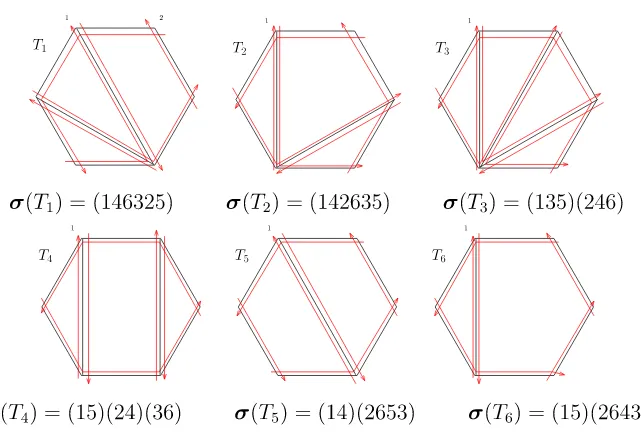
Fig. 2 Examples of tilings, their strand diagrams and permutations

Fig. 3 Tilings of the pants surface. Hereκ(S,M)=6×0+3×3+2×0+3−6=6

2 Definitions and results

Given any manifoldXwe write∂Xfor the boundary and(X)forX\∂X. For a subset

D⊂Xwe writeDfor its closure [23].

Amarked surfaceis an oriented 2-manifoldS; and a finite subsetM. Set M_∂ = M ∩∂S. An arc in marked surface (S,M) is a curve α in S such that(α) is an embedding of the open interval in(S)\M;∂α⊆M; and ifαcuts out a simple diskD

fromSthen|M∩D|>2.

Two arcsα, βin(S,M)arecompatibleif there exist representativesαandβin their isotopy classes such that(α)∩(β)= ∅.

Aconcrete tilingof(S,M)is a collection of pairwise compatible arcs that are in fact pairwise non-intersecting. Atiling T is a boundary-fixing ambient isotopy class of concrete tilings—which we may specify by a concrete representative, with arc set

E(T)(it will be clear that this makes sense on classes). Atileof tilingTis a connected component ofS\ ∪_α∈E₍T₎α. We writeF(T)for the set of tiles. (Note that ifSis not

homeomorphic to a disk then a tile need not be homeomorphic to a disk. For example a tile could be the whole ofSin the case of Fig.3.)

Fixing(S,M), it is a theorem that there are finite maximal sets of compatible arcs. Setκ(S,M) = 6g+3b+2p+ |M| −6, whereg is the genus,b the number of connected components of∂S, and p = |M∩(S)|. Supposeκ(S,M)≥1 and every boundary component intersects M. Then T maximal has|E(T)| = κ(S,M), and

every tile is a simple disk bounded by three arcs. Evidently given a tilingT then the removal of an arc yields another tiling. In this sense the set of tilings of(S,M)forms a simplicial complex, denotedA(S,M).

We say two tilings are related by ‘flip’ if they differ only by the position of a diagonal triangulating a quadrilateral. The transitive closure of this relation is called

f li p equivalence. We write[T]for the equivalence class of the tilingT; and Æ(S,M)

for the set of classes of A(S,M).

2.1 The Scott map

LetL be a connected component of the boundary of an oriented 2-manifold, and P

a finite subset labeledp1,p2, . . . ,p_|P|in the clockwise order (a traveller alongPin

Fig. 4 Composing tiles and strand segments. Hereτ(d)(2)=6

of all these points is. . . ,pi,p+_i ,p_i−₊₁,pi₊1, . . .. That is, the interval(pi−,p+i )⊂L

contains only pi.

Given(S,M), letM±denote a fixed collection of umbral sets over all boundary components. A J or dan diagram d on(S,M)is a finite number of closed oriented curves inStogether with a collection ofn= |M_∂|oriented curves inSsuch that each curve passes from some p_i+to some p−_j inM±; and the collection of endpoints is

M±. Intersections of curves are allowed, but must be transversal. Writeτ(d)for the permutation of M_∂ this induces. That is, if p_i+ goes to p−_j ind thenτ(d)(i) = j. Diagramd is considered up to boundary-fixing isotopy. Let Pu(S,M)denote the set of Jordan diagrams.

Next we define a map−→σ : A(S,M)→Pu(S,M). Consider a tilingT inA(S,M).

By construction each boundaryLof a tiletis made up of segments of arcs, terminating at a set of pointsP. Hence we can associateP±toPas above. To arc segmentspassing from pi topi₊1say, we associate astrand segmentαs intpassing from pi++1topi−,

such that the part of the tile on thesside of strand segmentαs is a topological disk.

Finally strand segment crossings are transversal and minimal in number. See tiletin Fig.4for example.

It will be clear that if two tiles meet at an arc segment then the umbral point constructions from each tile can be chosen to agree: as in Fig.4. Applying theαs

construction to every segmentsof every tiletinT, we thus obtain a collection−→σ(T)

of strand segments inSforming strands whose collection of terminal points are at the umbral points of∂S; so that−→σ(T)∈Pu(S,M). Altogether, writingMfor the set of

permutations of setM, we haveσ : A(S,M)→M_∂ defined by

σ =τ◦ −→σ (1)

We call this the Scott map. It agrees with Scott’s construction [30] in the case of triangulations of simple polygons.

The focus of this article is the case where(S,M)is a polygonP withnvertices. We write Anfor A(S,M)in this case, Ænfor Æ(S,M), and Punfor Pu(S,M). Our

main result can now be stated:

Theorem 2.1 Let T1,T2∈ Anbe tilings of an n-gon P. Thenσ(T1)=σ(T2)if and only if[T1]= [T2].

Sections3,4,5and6are concerned with the proof of this result.

We will see in Lemma3.5that−→σ(An)lies in the subset of Punof alternating strand

diagrams [26, §14]. Theorem2.1is thus related to Postnikov’s result [26, Corollary 14.2] that the permutations arising from two alternating strand diagrams are the same if and only if the strand diagrams can be obtained from each other through a sequence of certain kinds of ‘moves’. Consider the effect of a flip on the associated strands:

Comparing with Figure 14.2 of [26], the diagram shows that the flip corresponds to a certain combination of two types of Postnikov’s three moves (see Fig.19). Thus, [26, Corollary 14.2] may be used for the “if” part of Theorem2.1.

Remark 2.2 Theorem2.1does not hold as stated for arbitrary surfaces. For example, if T is a tiling of an annulus (S,M), then the Dehn twist of T induces the same permutation as T, regardless of the tile sizes. Similarly, if we consider tilings of punctured discs, the Scott map is invariant under certain rotations about the puncture.

2.2 Notation for tilings of polygons

We note here simplifying features of the polygon case that are useful in proofs. Geometrically we may consider a tile as a subset of polygon P considered as a subset ofR2. This facilitates the following definition.

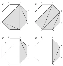
Definition 2.3 LetT ∈ An. By Tr(T)⊂R2we denote the union of all triangles in

T. We callT1andT2tr i angulat ed−par t equivalentif Tr(T1)=Tr(T2)and they agree on the complement of Tr(T1). See Fig.5.

By Hatcher’s Corollary in [14], two tilings are flip equivalent if and only if they are triangulated-part equivalent. The following is immediate.

Fig. 5 Tilings of an octagon, and the associated Tr(Ti). Note thatT1,T2are triangulated-part equivalent,

butT3,T4are not

Fig. 6 Examples of tilings, strands and Scott maps

Writen= {1,2, . . . ,n}for the vertex set ofP, assigned to vertices as for example in Fig.6. The ‘vertices’ ofAnas a simplicial complexare then(n−3)/2 diagonals. A diagonal between polygon verticesi,jis uniquely determined by the vertices. We write

its set of diagonals. Example: The tiling fromA8in Fig.1isT = {[2,8],[3,5],[5,8]}. An example of a top-dimensional simplex (triangulation) in A8of which thisT is a face isT ∪ {[3,8],[6,8]}.

Equally usefully, focussing instead on tiles, we may represent a tilingT ∈ An as a subset of the power setP(n): forT ∈ P(n)one includes the subsets that are the vertex sets of tiles inT.

Example 2.5 In tile notation the tiling fromA8in Fig.1becomes

T = {{1,2,8},{2,3,5,8},{3,4,5},{5,6,7,8}}

In this representation, whileA3= {{{1,2,3}}}, we have:

A4= {{{1,2,3,4}}, {{1,2,3},{1,3,4}}, {{1,2,4},{2,3,4}}}

We present two proofs of Theorem2.1: one by constructing an inverse—in Sect.4 we show how to determine the flip equivalence class from the permutation; and one by direct geometrical arguments—see Sect.6. We first establish machinery used by both.

3 Machinery for proof of Theorem

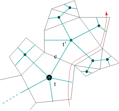
2.1

Theopen dualγ (T)of tilingT is the dual graph ofT regarded as a plane-embedded graph (see e.g. [7]) excluding the exterior face (so restricted to vertex setT). See Fig.7 for an example.

Lemma 3.1 Graphγ (T)is a tree.

Proof Let e be a diagonal of T and P the underlying n-gon. Then P\e has two

components. Thus removing a single edge separatesγ (T).

Aproper tilingis a tiling with at least two tiles. Anearin a proper tilingT is a tile with one edge a diagonal. Anr-ear is anr-gonal ear.

Corollary 3.2 Every proper tiling has at least 2 ears.

3.1 Elementary properties of strands

Consider a tilingT. Note that a tilet inT and an edgeeoft determine a strand of the−→σ(T)construction—the strand leavingt throughe. Now, when a strandsleaves a tile t through an edgee it passes to an adjacent tilet (as in Fig. 7), or exits P

and terminates. We associate a (possibly empty) branch γt,e ofγ (T)to this strand

ate: the subgraph accessible from the vertex oft without touchingt. Note that the continuation of the strandsleavestat some edgeedistinct frome, and thatγt,e is

Fig. 7 Dual tree example

Lemma 3.3 Consider the strand construction on a tiling. After leaving a tile a strand does not return.

Proof Consider the strand as in the paragraph above. If the strand exits the polygon

P atewe are done. Otherwise, since the sequence of graphsγti_,ei associated to the passage of the strand is a decreasing sequence of graphs, containing each other, it eventually leaves P and terminates in some tile of a vertex ofγt,e and so does not

return tot.

An immediate consequence of Lemma3.3is the following:

Corollary 3.4 A strand of a tiling T can only use one strand segment of a given tile of T .

Lemma 3.5 Let T ∈ An be a tiling of an n-gon. Then the strands of−→σ(T)have the following properties[26, §14]: (i) Crossings are transversal and the strands crossing a given strand alternate in direction. (ii) If two strands cross twice, they form an oriented digon. (iii) No strand crosses itself.

Proof The first two properties follow from the construction. That no strand crosses itself follows from Corollary3.4. Note that the underlying polygon can be drawn convex, in which case strands are left-turning. The requirement that there are no unoriented digons follows from the fact that strands are left-turning in this sense. (Remark: our main construction is unaffected by non-convexity-preserving ambient isotopies, but the left-turning property is only preserved under convexity preserving

maps.)

We writex yfor a strand starting at vertexx and ending at vertexy. Thus if

Fig. 8 Strands with their antistrands

emphasise that verticesx1,x2,x3are ordered minimally clockwise, we will repeat the “smallest” element at the end:x1<x2<x3<x1.

Definition 3.6 Letq be a vertex of a polygon with strand diagram.

(1) We say that a strandx y covers q if we havex < q < y < x minimally clockwise.

(2) We say that x y covers strand x y if x < x < y < y < x or

x <y<x<y<x.

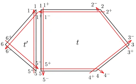
3.2 Factorisation Lemma

Consider the two strandss1,s2 passing through an edgeeof a tilet. We say these strands are ‘antiparallel ate’; and consider the ‘parallel’ strands1and antistrands2

both moving intotfrome. See Fig.8for examples.

Lemma 3.7 (‘Lensing Lemma’)(I) Let strand segments s1and s2be antiparallel at an edge e of a tile t in a polygon tiling T . Traversing the two segments in the direction from e into the tile t , they do one of the following: (a) if t is a triangle the segments cross in t and do not meet again; (b) if t is a quadrilateral the segments leave t antiparallel in the opposite edge; (c) if|t|>4they leave t in different edges and the strands do not cross thereafter.

(II) In any polygon tiling T , two strands cross at most twice. If two strands cross twice then (i) they pass through a common edge e; (ii) the crossings occur in triangles, on either side of e, with only quadrilaterals between.

Proof (I) See the Fig.8. Note that in cases (a) and (c) the strands pass out oftthrough different edges and hence into different subpolygons. Now use Lemma3.3. (II) Every crossing has to occur in a tile. If two strands enter a tile across different edges, they have not crossed before entering into the tile (Lemma3.1). The claim then follows

from (I).

Lemma 3.8 Let T be a tiling of an n-gon and σ = σ(T). Then (a)σ has no fixed points and (b) there is no i withσ (i)=i+1.

Fig. 9 Schematic for two strands passing through diagonale= [i,j]

before leaving this tile at a vertex different fromi. By Lemma3.3, it never returns back to the tile. (b) Consider the tile with edgee= [i,i+1]. The strand starting at

i and the strand ending ati+1 have segments in the same tile and hence differ by

Corollary3.4.

Lemma 3.9 (‘Factorisation Lemma’)Let P be a polygon and T1,T2two tilings of P. Assume that there exists a diagonal e= [i,j]in T1and T2. Denote by Pthe polygon on vertices{i,i+1, . . . ,j−1,j}. We have:

σ(T1)=σ(T2)⇒σ(T1|P)=σ(T2|P).

Proof Consider Fig.9. The only way a strand of−→σ(T1)passes out ofPis throughe, and there is exactly one such strand (and one passing in). This strand is non-returning by Lemma3.3, so its endpoints are identifiable fromσ =σ(T1)as the unique vertex pairk,lwithσ (k)=land withkinPandlnot. Apart from this and the corresponding ‘incoming’ pair withσ(k)=l, all other strand endpoint pairs of−→σ(T1|P)are as in

−

→_{σ(T1)and hence agree with}−→_σ(T2|

P)ifσ(T1)=σ(T2). Indeed, ifσ(T1)=σ(T2)

thenσ(T2)identifies the same two pairsk,landk,l. At this point it is enough to show that the image of vertexkunder−→σ(T1|P), which is either vertexi or j, is the same as for−→σ(T2|P). But it isi in both cases since the strand passing out ofPthroughe

is ati.

3.3 Properties of strands and tiles

We will say that a vertex in polygonPissimplein tilingT if it is not the endpoint of a diagonal. We will say that an edgee= [i,i+1]ofPis asimple edgeinT if both vertices are simple.

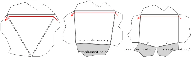
Fig. 10 Tiles with complementary edges and their complements

Proof If[i,i+1]is simple inT, the claim follows by construction. Ifiis not simple, then the strand ending aticontains the strand segment of the diagonal[j,i]ofT with

j<i−1 maximal clockwise and has starting point in{j,j+1, . . . ,i−2}. Similarly, ifi +1 is not simple, the strand starting ati+1 contains the strand segment of the diagonal[i+1,k]withk>i+2 minimal anticlockwise. Its ending point is among

{i+3, . . . ,k}.

In general a strand passes through a sequence of tiles. At each such tile it is parallel to one edge and passes through the two adjacent edges. Any remaining edges in the tile are calledcomplementaryto the strand. Each of these complementary edges defines a sub-tiling—the tiling of the part ofPon the other side of the edge. We call this the

complement to the corresponding edge. Note that the strand covers every vertex in this sub-tiling. See for example Fig.10. We deduce:

Lemma 3.11 (I) A strand ii+2passes only through triangles.

(II) A strand i i+3passes through one quadrilateral (with empty complement) and otherwise triangles.

(III) A strand i i +4passes through one quadrilateral (with a complementary triangle) or two quadrilaterals or one pentagon (with empty complement), and otherwise triangles.

(IV) A strand ii+k passes through a tile sequence Qisuch that

k−2≥

i

(|Qi| −3)

(the non-saturation of the bound corresponds to some tiles having non-empty complement).

Example 3.12 As an illustration for Lemma3.11consider Fig.6. Both tilings have a strand 69, illustrating the casek=3.

In the tiling on the left, there is a strand 13 3 passing through one quadrilateral with complementary triangle{14,1,2}.

Proof If:Thas a strand direct fromi toi +2 in the given ear. Note that all other tilings in[T]have only triangles incident ati+1 (since a neighbourhood ofi+1 lies in the triangulated part). One sees from the construction that these tilings all have a strand fromi toi+2. See (a):

(a) (b)

(Note that Postnikov’s result [26, Corollary 14.2] and the strand/flip construction in Sect.2.1also implies the “if” part. For self-containedness we will avoid assuming Postnikov’s result.)

Only if: If there is no suchTin[T] then among the tiles incident ati +1 is one with orderr>3. The strand fromi passes intoPat the first tile incident ati+1. If this is a triangle then the strand passes into the second tile incident ati +1, and so on. Thus eventually the strand meets a tile of higher order—see (b) above. But then

by Lemma3.11we haveii+kwithk>2.

For givennlet us writeτ for the basic cycle element inn:τ =(1,2, . . . ,n). The

following is implicit in [30], and is a corollary to Lemma3.11.

Lemma 3.14 For T ∈ An,σ(T)=τ2if and only if T is a triangulation.

Definition 3.15 Arunis a subsequence of formi−1,i−2, . . . ,i−r+1 in a cycle of a permutation ofn. A maximal subsequence of this form is anr-run at i.

In Fig.6, both permutations have a 3-run at 9.

Lemma 3.16 Let T ∈ An, andσ =σ(T). We have

(i) σcontains a cycle of length≥r , where r ≥2, with an r -run at j⇐⇒ [j−1,j−2],

[j−2,j−3], . . . ,[j−r+2,j−r+1]is a maximal sequence of simple edges in T ;

(ii) Assumeσ is as in (i) and r<n−1. Then TFAE

(a)[j −r,j] ∈ T ; (b){j −r,j −r +1, . . . ,j}is an(r+1)-ear in T ; (c)

σ (j−r)= j .

Note that the caser=2 occurs if j−1 is simple, while the edge[j−1,j−2]is not simple—a triangular ear.

Proof (i) Follows from Lemma3.10.

(ii) Observe that the the assumptions in (ii) are consistent with (b). (a)⇒(b) follows from the assumptions. (b)⇒(c) follows from the construction.

To show (c)⇒(a) first note that by the assumptions, j and j −r are not simple. Among the diagonals incident with jconsider the diagonal[j,q1]maximal clockwise from j. Among the diagonals incident with j−rconsider the diagonal[q2,j −r]

Ifq1= j−r(and henceq2= j), we are done. So assume for contradiction that

j <q1≤q2< j−r < j. Both diagonals are edges of a common tileQcontaining the simple edges[j−1,j−2],[j−2,j−3], . . . ,[j−r+2,j−r+1]. Consider the strand starting at j −r. It leaves the tile Qat an edge atq2. By Corollary3.4it cannot return back intoQ, and so its endpoint is different from j.

4 Inductive proof of Theorem

One proof strategy for the main theorem (Theorem2.1) is as follows. We assume the theorem is true for ordersm<n(the induction base is clear).

The ‘If’ part follows from the Factorisation Lemma (Lemma3.9) and Lemma3.14. For the ‘Only if’ part proceed as follows. ConsiderT1,T2withσ =σ(T1)=σ(T2).

Note thatT1has an ear, either triangular or bigger (Corollary3.2). Pick such an ear

E. Consider the cases (i)|E| =3; (ii)|E| =3.

(i) IfEis triangular inT1thenσ =σ(T1)hasii+2 at the corresponding position. Thus so doesσ(T2)=σ(T1), and hence there is aT₂in[T2]also with this ear, by Lemma3.13. Note thatσ(T₂)=σ(T2)sinceT₂∼T2.

Since T1\E and T₂\E are well defined we have σ(T1\E) = σ(T₂\E)by the Factorisation Lemma (Lemma3.9). That is, the Scott permutationsσ(T1)andσ(T₂)

ofT1andT₂agree on the part excluding this triangle. But then[(T1\E)]= [(T₂\E)]

(i.e. the restricted tilings agree up to triangulation) by the inductive assumption. Adding the triangle back in we have[T1] = [T₂]. But[T₂]= [T2]and we are done for this case.

(ii) If earEis not triangular inT1thenT2has an ear in the same position by Lemma3.16. The argument is a direct simplification of that in (i), consideringT1\E andT2\E.

5 Geometric properties of tiles and strands

Definition 5.1 Fixn. Then an increasing subsetQ= {q1,q2, . . . ,qr}of{1,2, . . . ,n}

defines two partitions:

I(Q)= {[q1, . . . ,q2),[q2, . . . ,q3), . . . ,[qr, . . . ,q1)} J(Q)= {(q1, . . . ,q2], (q2, . . . ,q3], . . . , (qr, . . . ,q1]}

We denote the parts by Ii(Q) := [qi, . . . ,qi₊1)and Ji(Q) := (qi, . . . ,qi+1], for i =1, . . . ,r.

Such partitions arise from tilings: LetQ∈T ∈ An. Then the vertices ofQpartition the vertices ofPin two ways. Consider the edgee= [qi,qi₊1]ofQ. In the subpolygon on the verticesqi,qi +1, . . . ,qi₊1, there areqi+1−qi strands of−→σ(T)starting at

vertices in Ii(Q)and the same number of strands ending at the vertices in Ji(Q).

Among them,qi₊1−qi−1 remain in the subpolygon.

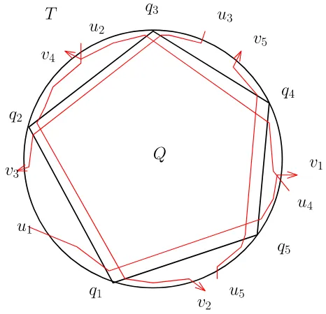
Fig. 11 Tile inducing partition and long strands forQ

Using this notation, we get an alternative proof for Corollary3.4stating that a strand of a tiling can only use one strand segment of a given tile: LetQbe a tile of a tiling

T ∈ Anand letq1, . . . ,qr be its vertices,r ≥3,q1<q2<· · ·<qr <q1. Assume strandx y involves a strand segment of Q, say parallel to the edge [qi₋1,qi].

By construction, this strand segment is oriented from qi to qi₋1, comes from the

subpolygon on the verticesqi,qi+1, . . . ,qi₊1and then passes into the subpolygon

on the verticesqi₋2,qi−2+1, . . . ,qi−1. We claim that the strand then necessarily starts

inIi(Q)and ends inJi₋2(Q), i.e. thatx=qi+1andy=qi−2. We show that it ends in Ji₋2(Q): Consider the subpolygon on the verticesqi−2,qi−2+1, . . . ,qi−1, bounded

by the edge[qi₋1,qi]. From the orientation of strand segments in tiles, it is clear, that

the strand then leaves this subpolygon nearzwherez∈ {qi₋2+1, . . . ,qi−1−1}is

the first vertex met when going fromqi₋2towardsqi₋1which has an edge[z,qi₋1].

Hencey∈Ji₋2(Q). A similar argument showsx ∈Ii(Q).

Remark 5.2 LetT be a tiling of P, with tile Qinducing partitions as above. There are two types of strands regarding these partitions. Letx ybe a strand starting in

Ii1(Q)and ending inJi2(Q)for somei1,i2. Then we either havei1=i2ori1=i2+2 (by the preceding argument or by Corollary3.4). The casei1=i2+2 is illustrated in Fig.11forQa pentagon.

Lemma 5.4 Let Q be an r -tile of a tiling of P with vertices q1 < · · · < qr < q1 clockwise. Then every long strand x y with respect to Q covers exactly r−2

vertices of Q and there are exactly two vertices qi₋1,qi for every such strand with y≤qi₋1<qi ≤x<y (clockwise).

Proof Ifsis a long strand forQwithxy, then there existsisuch thatx∈Ii(Q)= [qi, . . . ,qi₊1)and y ∈ Ji−2(Q) = (qi−2, . . . ,qi−1] (reducing the index modn),

hence it coversqi₊1,qi+2, . . . ,qi−2. For an illustration, see Fig.11.

6 Geometric Proof of Theorem

We now use geometric properties of tilings to prove the “only if” part of Theorem2.1. The maximum tile size of tilingT is denotedr(T). For two tilingsT1,T2andri = r(Ti), the caser1 = r2is covered in Corollary6.3; andr :=r1 =r2follows from Lemma6.4. We first prove an auxiliary result.

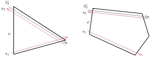
Lemma 6.1 (a) Consider a tiling T in Anwith a diagonal e= [s1,s2]. For each vertex q with s1<q <s2 <s1, there exists a strand s : y z in−→σ(T)covering q, with s1≤ y<q <z≤s2<s1.

(b) Consider T,q,s as in (a) and a further tiling T of P containing a tile Q such thatdim(Q∩e)=1and q∈ Q. Ifσ(T)contains a strand with yz as in (a), it is a long strand for Q (as defined in Definition5.3).

Proof (a) Lete = [n1,n2]be the shortest diagonal inT lying aboveq. Note,s1 ≤ n1<q<n2≤s2<s1. Consider the strand segment inσ(T)followingefromn1to

n2(see figure below). This induces a strandswithyz, say. We claimn1≤y<q

andq < z ≤ n2. To see this let[x,n1] be in T withn1 ≤ x < n2,x maximal (x=n1+1 possibly). Thenx≤qsinceeis the shortest diagonal aboveqand sos

has its starting point among{n1,n1+1, . . . ,x−1}. A similar argument proves the claim fory.

Lemma 6.2 Letσ(T1)=σ(T2). If in T1there exists an edge e= [s1,s2]and in T2a tile Q of size≥4withdim(Q∩e)=1, then either e is an edge of Q or e separates vertices of Q (s1>qx >s2>qy >s1for some x,y) and|Q| =4.

Proof Ifeis not an edge ofQ, we find verticesqi andqj of Qwiths1<qi <s2< qj <s1. We can thus use Lemmas5.4and6.1forqi and again forqj to see thatQ

hasr−2 vertices on the left side ofeandr−2 vertices to the right ofe, and that they all differ froms1and froms2, wherer= |Q|. Sor =2(r−2)andr=4.

Corollary 6.3 Let T1and T2be two tilings of a polygon P withσ(T1)=σ(T2). Then r1=r2.

Proof Letr = r2. Assume thatσ(T1) = σ(T2). In caser1 = 3, the claim follows from Lemma3.14: in this case,σ(T1)is induced byi → i+2 andT2 has to be a triangulation, too. Assume for contradiction thatr1<r. Since we can assumer1>3, we haver >4. We consider a tileQof sizer>4 inT2, with verticesq1, . . . ,qr. InT1, we choose a tileSwith dim(Q∩S) >1. ThenShas an edgeewith dim(Q∩e)=1 and so by Lemma6.2,Qis a tile ofT1, a contradiction to the maximal tile size inT1.

Lemma 6.4 Let T1and T2be two tilings of a polygon P with σ(T1) = σ(T2)and assume r1=r2=4. Then[T1]= [T2].

Proof By Lemma3.10the positions of 4-ears inT1andT2agree, whenr1=r2=4. By the Factorisation Lemma (Lemma3.9) we can remove (common) ears of size 4, to leave reduced tilingsT₁ andT₂ of some P. These necessarily have ears, but by Lemma3.11, (up to equivalence) 3-ears can be chosen to be in the same positions in

each tiling. Now iterate.

Proof of Theorem2.1 If the maximum tile sizes ofT1and ofT2differ, the claim follows from Corollary6.3. So letr =r1=r2be the maximum tile size ofT1and ofT2. If

r =4, Lemma6.4proves the claim. So assume that there are tiles of sizer >4 and consider such a tileQinT2. By Lemma6.2there are no diagonals ofT1‘intersecting’

Q, so inT1we have a tile containingQ. Applying the same argument with the tilings reversed we see thatT1andT2agree on parts tiled with tiles of size>4.

By the Factorisation Lemma (Lemma3.9), we can remove all (common) ears of size>4. Among the remaining (common) tiles of size at least 5, we choose a tileQ

and a non-boundary edgeeofQ, such that to one side ofe, all tiles inT1and inT2have size at most four. LetPbe the union of these tiles of size≤4. By the Factorisation Lemma we haveσ(T1 |P)=σ(T2 |P)and by Lemma6.4,[T1 |P] = [T2|P].

We can remove Pand repeat the above until Qis a (common) ear - which can be

removed, too. Iterating this proves the claim.

7 On the image of the Scott map treated combinatorially

To give an intrinsic characterization of the image innof the Scott mapσ : An→n

does not equip the image with a group structure (or indeed any algebraic structure). Here we report on one invariant which Theorem2.1gives us access to, namely the size of the image, which is given by|Æn|.

As an initial illustration we observe that:

Proposition 7.1 The number of permutations arising from tiling an n-gon using one r -gon (r>3) and triangles otherwise isn_r.

Proof By the main Theorem this is the same as enumerating the classes in Ænof this

type. Since the details of the triangulated part are irrelevant, the class is determined by choosing the vertices of ther-gon. Hence choosingrfromn.

Example 7.2 In total, there are 26 permutations arising from the 45 tilings of the hexagon: one from the empty tiling; 6 from tilings with one pentagon and one triangle; 15 from tilings with one quadrilateral and two triangles; 3 from tilings using two quadrilaterals; and 1 from the triangulation case.

Figure2contains examples of these tilings and the associated permutations. In order to go further we will need some notation.

7.1 Notation and known results

Recall that an integer partitionλ=(λ1, λ2, . . . )has also the exponent notation:

λ=rαr(r−1)αr−1· · ·₂α2₁α1

whereαi is the number of parts inλequal toi. Aλ-tilingis a tiling with, for eachd,

αdtiles that are(d+2)-gonal.

Recall that An is the complex of tilings of the n-gon. Definean = |An|. Write

An(m)(withm∈ {0,1,2, . . . ,n−3}) for the set (andan(m)the number) of tilings withm diagonals. Write An(λ) (withλan integer partition ofn−2) for the set of λ-tilings (thus with am-gonal face for each rowλi =m−2). Thus

An(m) =

λn−2:λ₁=m+1

An(λ) (2)

whereλdenotes the conjugate partition toλ[21], soλ₁is the number of parts. Similarly recall Ænis the set of classes of tilings under triangulated-part/flip

equiv-alence. Write Æn(m)for the setAn(m)under triangulated-part equivalence and Æn(λ)

the setAn(λ)under triangulated-part equivalence.

(7.3)The sequenceanis the little Schröder numbers (see e.g. [31] and OEIS A001003). It is related to the Fuss–Euler combinatoric as follows. By [28] the number of tilings of then-gon withmdiagonals is

an(m)= 1 m+1

n+m−1

m

n−3

m

(an(m)=qm(1,n)from [28]). Thus in addition to the usual generating function

n≥0

anxn=1+x− √

1−6x+x2

4x

we have

an= n

m=0

1

m+1

n+m−1

m

n−3

m

(4)

7.2 Explicit construction ofA_n

Of greater use than an expression for the size of Anis an explicit construction of all tilings. For this we shall consider a tiling in Anto be as in the formal definition, i.e. to be the same as its set of arcs. This is the set of diagonals in the present polygon case, where we can represent an arc between verticesi,j unambiguously by[i,j]. In particular then we have an inclusion An₋1 → An. The copy of An−1 in An is

precisely the subset of tilings in which vertexn is simple and there is no diagonal

[1,n−1].

There is a disjoint imageJ(An₋1)of An−1inAn given byJ(T)=T ∪ {[1,n−

1]}. The set An₋1 J(An−1)is the subset of An of elements in whichn is simple.

Consider in the complement the subset of tilings containing[n−2,n]. In this the vertexn−1 is necessarily simple. Thus this subset is the analogue Jn₋1(An−1)of J(An₋1)constructed withn−1 instead ofnas the distinguished simple vertex. The

practical difference is that (i) the image tilings have all occurences ofn−1 replaced byn; (ii) the ‘added’ diagonal is[n−2,n].

There remain inAnthe tilings in whichnis not simple but there is not a diagonal

[n−2,n]. Consider those for which there is a diagonal[n −3,n]. In the presence of this diagonal any tiling ‘factorises’ into the parts in the two subpolygons on either side of this diagonal. One of these has vertices 1,2, . . . ,n−3 andn, and so its tilings are an image of An₋2where vertexn−2 becomes vertexn. The other has vertices n−3,n−2,n−1,nand so has tilings from a shifted image ofA4, but hasnsimple (since[n−3,n]is the first diagonal in the original tiling). Since n is simple, it is the part of that image coming from A3 J(A3). We write 2.K(A3)for these two shifted copied of A3. We write 2.K(A3)·An₋2for the meld with tilings from An−2

to construct the set of tilings of the original polygon.

There now remain inAnthe tilings in whichnis not simple but there is not a diagonal

[n−2,n]or[n−3,n]. Consider those for which there is a diagonal[n−4,n]. In the presence of this diagonal any tiling ‘factorises’ into the parts in the two subpolygons on either side of this diagonal. We have the obvious generalisation of the preceeding construction in this case, written 2.K(A4)·An₋3.

Proposition 7.4 Consider the list defined recursively byA3=(∅)and

An = An₋1∪J(An−1)∪Jn−1(An−1)∪ n−3

r=2

2.K(Ar₊1)·An−r

where set operations on lists are considered as concatenation in the natural order;

2.−denotes the doubling as above; K()denotes the relabeling of all vertices so that the argument describes a suitable subpolygon; and A·B denotes the meld of tilings from subpolygons as above. Then this list is precisely a total order of An.

Proof Noting the argument preceding the Proposition, it remains to lift the construc-tion from the set to the list. But this requires only the interpretaconstruc-tion of union as

concatenation.

7.3 Tables forA_n()

The class sets Æn are harder to enumerate than An. Practically, one approach is to

list elements of An and organise by arrangement of their triangulated parts, which determines the class size. We first recall the numbersan(m)of tilings of ann-gon with

mdiagonals: see Table1. The main diagonal enumerates the top dimensional simplices in An. It counts triangulations and hence is the Catalan sequenceCn. The entries in the next diagonal correspond to tilings with a single quadrilateral and triangles else.

We will give the number of elements of Æn(m)for smallnin Table2. In order to

verify this it will be convenient to refine Tables1and2by considering these numbers for fixed partitions λ. Specifically we subdivide each case ofm from the previous tables according toλ, with them-th composite entry written as a list of entries in the form (λ1,λ2,...)

an(λ) ranging over allλwith|λ| =m. Thus for example

(32₎

7 tells that a7((3,2))=7. We include Table3for An(λ)and Table4for Æn(λ). Neither table

is known previously. Theancase is computed partly by brute force (and see below); verified in GAP [32], and checked using identity (2)).

Table 1 Values ofan(m), and hencean, in low rank

n m=0 1 2 3 4 5 6 7

3 1 1

4 3 1 2

5 11 1 5 5

6 45 1 9 21 14

7 197 1 14 56 84 42

8 903 1 20 120 300 330 132

9 4279 1 27 225 825 1485 1287 429

10 20,793 1 35 385 1925 5005 7007 5005 1430

n 1 n(n₂−3) (

n+1 2 )(

n−3 2 )

Table 2 Table of Ænsizes up ton=10

n m=0 1 2 3 4 5 6 7

3 1 1

4 2 1 1

5 7 1 5 1

6 26 1 9 15 1

7 100 1 14 49 35 1

8 404 1 20 112 200 70 1

9 1691 1 27 216 654 666 126 1

10 7254 1 35 375 1660 3070 1902 210 1

For the purpose of computing Æn a better filtration is by the partition describing

the size of the connected triangulated regions. But this is even harder to compute in general.

7.4 Formulae for|Æ_n()|for alln

In theλnotation Proposition7.1becomes

|Æn((r−2)1n−r)| =

n r

(5)

To determine the size of image of the Scott map for a polygon of a given rank, one strategy is to compute Æn(λ)through An(λ). While An(λ)is also not known in

general, we have a GAP code [3,32] to compute any given case.

If in a tiling, there is at most one triangle, we have Æn(λ)∼= An(λ). In the case of

two triangles, the following result determines|Æn(λ)|from tilings of the same type

and from tilings where the two triangles are replaced by a quadrilateral:

Proposition 7.5 Letλ=rαr(r−1)αr−1· · ·₂α2₁α1_.

(i) Ifα1<2then|Æn(λ)| =an(λ).

(ii) Ifα1=2then

|Æn(λ)| = an(λ)−(α2+1)an(λ21−2)

(iii) Ifα1=3then

|Æn(λ)| =an(λ)−(α2+1)an(λ21−2)+(α3+1)an(λ31−3)

(iv) Ifα1=4then

|Æn(λ)| =an(λ)−(α4+1)an(λ41−4)+(α3+1)an(λ31−3) +

α2+2

2

Table

3

T

able

for

size

of

An

Table

4

T

able

for

size

of

Æ

n

Proof (ii) Consider partitioning A = An(λ) into a subset A of tilings where the triangles are adjacent, and A where they are not. Evidently|Æn(λ)| = |A|/2+ |A| = |A| − |A|/2. On the other hand in A the triangles form a distinguished quadrilateral. For each element of An(λ21−2)we get α2+1 ways of selecting a

distinguished quadrilateral. There are two ways of subdividing this quadrilateral, thus

|A| =2(α2+1)an(λ21−2), and so (ii) is proved.

Example 7.6 Proposition7.5determines|Æ8(2212)|. Here A8(2212)gives an

over-count because of the elements where the two triangles are adjacent. Only one representative of each pair under flip should be kept. These are counted by mark-ing one quadrilateral in each element of A8(23). There are three ways of doing this,

so we have

|Æ8(2212)| = |A8(2212)| −3|A8(23)| =180−36

from Table3. Similarly|Æ8(412)| = |A8(412)| − |A8(42)| =36−8.

(7.7)Proof of (iii):Forα1 = 3 partition A = An(λ)into subset A of tilings with

three triangles together; A with two together; and A with all separate. We have

|Æn(λ)| = |A| + |A|/2+ |A|/5. That is,

|Æn(λ)| = |A| − |A|/2−4|A|/5. (6)

Considering the triangulated pentagon in a tilingT inAas a distinguished pentagon we have

|A| =5(α3+1)an(λ31−3). (7)

Next aiming to enumerate A, considerλ21−2, somewhat as in the proof of (ii), but here there is another triangle, which must not touch the marked 4-gon. Let us write (α2+1)A(λ21−2)to denote a version ofA(λ21−2)where one of the quads is marked.

There are two ways of triangulating the marked quad, givingX =2(α2+1)A(λ21−2),

say. Consider the subsetBofXof tilings where the marked quadrilateral and triangle are not adjacent.

Claim:B∼=A.

Proof The construction (forgetting the mark) defines a map B → A. Marking the adjacent pair of triangles in an element ofAgives a map A→ Bthat is inverse to

it.

The complementary subsetCofXhas quadrilateral and triangle adjacent. Elements map intoAby forgetting the mark.

Claim:Cdouble counts A, i.e. the forget-map is surjective but not injective.

AltogetherA=B=X−C=X−2Aso

Æ(λ)= A(λ)−((1/2)X−A)−(4/5)A=A(λ)−(X/2)+A/5 = A(λ)−(α2+1)A(λ21−2)+(α3+1)A(λ31−3)

(7.8)Proof of (iv):Forα1 =4 partition A = A(λ)by A = A4+A31+A22+ A211+A1111so that

Æ=A4/C4+A31/C3+A22/C2₂+A211/C2+A1111=A−13

14A

4

−4

5A

31₋3

4A

22₋1

2A

211

By direct analogy with (7) we claim

A4=14(α4+1)A(λ41−4)

Next considerX =5(α3+1)A(λ31−3), marking one 5-gon, and then triangulating

it. We have a subsetBwhere the 5-gon and triangle are not adjacent; and complement

C.

Claim:B∼=A31. This follows as in the proof of part (iii). The complementCmaps toA4by forgetting the mark. Claim: 14|C| =30|A4_|.

Proof There are 6 ways the 5-gon and triangle can occupy a hexagon together, and 5 ways to triangulate the 5-gon. This gives 30 marked cases, which pass to 14 triangu-lations.

So far we have that

A31=B=X−C=5(α3+1)A(λ31−3)−

30 14A

4

It remains to determineA22_andA211_.

(7.9)Next considerY =4(α2+₂2)A(λ221−4), marking two 4-gons, and then

triangu-lating them. SubsetDhas the 4-gons non-adjacent; andEis the complement. Claim:D∼= A22. This follows similarly as the statement onB.

The complementEmaps toA4by forgetting the marks. Claim: 14|E| =12|A4|.

So far we have

A22 =Y −E =4

_α

2+2

2

A(λ221−4)−12 14|A

4_|

Next we needA211.

(7.10)Next consider Z = 2(α2+1)A(λ21−2), marking a 4-gon and triangulating

it. Subset Fhas the three parts non-adjacent. SubsetGhas the 4-gon and one trian-gle adjacent. SubsetGhas the two triangles adjacent. Subset H has all three parts adjacent:

Z =F+G+G+H

Claim:F∼= A211. This follows similarly as the statements onBand onC. The setGmaps toA31, andGtoA22, andHtoA4, by forgetting the marks. Claim: (a)|G| =2|A31|and (b)|G| =2|A22|and (c) 14|H| =42|A4|.

Proof (a) Elements ofGpass to tilings with triangulations of a 5-gon and a separate triangle. The collection of them triangulating a given 5-gon and triangle has order 10 (5 ways to mark a quadrilateral in the 5-gon, then two ways to triangulate it). On the other hand the number of triangulations of the same region inA31is 5. (b) Elements ofGpass to tilings with triangulations of two 4-gons. The collection

of such gives all these triangulations. Each one occurs twice in G since the triangulation of the two 4-gon regions can arise in G with one or the other starting out as the marked 4-gon.

(c) Elements of H pass to tilings with triangulations of a hexagon. The collection of such gives A6(212)= 21 ways of tiling the hexagon with quadrilateral and two triangles, then two ways of tiling the quad. On the other hand there are 14 triangulations of this hexagon inA4.

We haveA211=Z−(G+G+H)=2(α2+1)A(λ21−2)−(2₁A31+2₁A22+42₁₄A4).

Altogether now

Æ(λ)= A−13

14A

4₋4

5A

31₋3

4A

22₋1

2A

211

= A(λ)−13

14A

4₋4

5

5(α3+1)A(λ31−3)−

30 14A 4 −3 4 4

α2+2

2

A(λ221−4)−12

14|A

4_|

−1

2

2(α2+1)A(λ21−2)−

2 1A

31₊2

1A

22₊42

14A

4

= A(λ)+−13+21

14 A

4₊1

5

5(α3+1)A(λ31−3)−

30 14A 4 +1 4 4 _α

2+2

2

A(λ221−4)−12

14|A

4_|

−1

2

2(α2+1)A(λ21−2)

= A(λ)+−13−6−3+21

14 A

4_+(α

3+1)A(λ31−3)+

α2+2

2

A(λ221−4)

−(α2+1)A(λ21−2)

= A(λ)−(α4+1)A(λ41−4)+(α3+1)A(λ31−3)+

α2+2

2

A(λ221−4)

−(α2+1)A(λ21−2)

Remark 7.11 In [2] we prove the following generalisation of Proposition7.5

|Æn(λ)| =

μα1

(−1)α1−μ1 i≥2

_α

i +αi(μ)

αi(μ)

an(λμ1−α1)

whereμ=rαr(μ)(r−1)αr−1(μ). . .₂α2(μ)₁α1(μ)_.

7.5 Tables for Æ_n

Proposition 7.12 The numbersÆnfor n<11are given in Table2.

Proof The numbersan(λ)are given in Table3by a GAP calculation [3]. The num-bers in Table4 then follow from formula (5) and Proposition7.5. Table2 follows

immediately.

7.6 On asymptotics

We determined in Tables2,4 the sizes of the image of the Scott map in low rank. Of course the ratio of successive sizes of the formal codomains grows with n as

|n|/|n−1| =n. In the next table we consider the ratios of two consecutive entries

of the sequence|Æn|n.

n 3 4 5 6 7 8 9 10

|Æn| 1 2 7 26 100 404 1691 7254

|Æn|/|Æn−1| 2 3.5 3.71 3.85 4.04 4.19 4.29

(7.13)A paradigm for this is the Catalan combinatoricCn(see e.g. [31]), which can also be equipped with an inclusion in the permutationsn—see e.g. [19,29] (NB this

n 3 4 5 6 7 8 9 10

|Cn| 1 2 5 14 42 132 429 1430

|Cn|/|Cn−1| 2 2.5 2.8 3 3.14 3.25 3.33

This raises the question: Is there a limit rate in the Æncase?

8 On enumerable classes of strand diagrams and plabic graphs

LetPbnbe the set of reduced plabic graphs [26, §11] of rank-n; and Ponbe the set

of alternating strand diagrams as in [26, §14]. (See also Sects.8.1and 8.5.) Their relationship withAncan be summarized as follows:

An − →_σ G

Ptn Pbn D Pon

D

Xn

HereGis as in Sect.1,−→σ as in Sect.2.1, andD,Das in Sect.8.2. In this section we apply Theorem2.1to corresponding subsets of plabic and strand diagrams. We define the setsXnofmi ni mali ststrand diagrams, see Sect.8.1; andPtnofr hombi c

(plabic) graphs, see (8.5). We will show that these sets are in bijection with An. For the sake of brevity we refer to Postnikov’s original paper for motivations behind the constructions of plabic and strand diagrams themselves. These are large and com-plex classes of objects, and canonical forms for them would be a useful tool. The rigid/canonical nature of Aninduces canonical forms for (the restricted cases of) the other constructions.

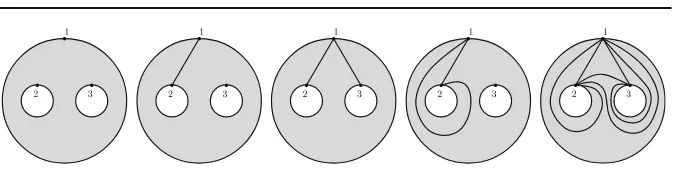
We start by characterizing the image of−→σ in Theorem8.4as the set of minimalist strand diagrams and hence show that−→σ is injective. In Sect.8.2we recall Postnikov’s bijections between alternating strand diagrams and plabic graphs. (An illustration of the connection between plabic graphs and strand diagrams is given by Fig.12b.) This allows us to characterize the image ofGin Sect.8.3as the set of rhombic plabic graphs, Theorem8.19. Finally we determine the images of flip equivalence in the two other realisations.

8.1 On−→and strand diagrams

Fig. 12 aA tilingT(black) with strand diagram−→σ(T)ofT;bthe plabic graphD(−→σ(T))(green)

Fig. 13 A Jordan diagram inX8and its image underf

Note that this agrees with the ordinary definition ofalt er nati ngstr anddi agr am

[4,26] forSa simple disk. Here rankn= |M_∂| = |M|.

For any directed planar graph we classify the faces as clockwise, counterclockwise, alternating or other.

(8.1)LetXn be the subset of rank-nalternating strand diagrams whose faces are as follows: (i)n clockwise faces at the boundary, labelled 1,2, . . . ,n going clockwise around the boundary; (ii) alternating faces with four sides; (iii) oriented faces in the interior that are counterclockwise and have at least 3 sides.

We call the elements ofXnmi ni mali st strand diagrams. See Fig.13for an example.

Fig. 14 Strands partition a tile into vertex, edge and face parts

(8.3)We define a ‘shrink’ mapf : Xn → An as follows: Let d ∈ Xn. Note from (8.2) that ind regarded as an isotopy class of concrete diagrams there are cases in which all the edges of clockwise faces are arbitrarily short. Thus the clockwise faces are arbitrarily small neighbourhoods ofnpoints; and alternating faces have two short edges and two edges that pass between the clockwise faces (and hence are not short). The paths of non-short edges are not constrained by the ‘shrinking’ of the clockwise edges. Thus each pair may be brought close to each other, and hence form an arbitrarily narrow neighbourhood of a line between two of thenpoints. Since no two alternating faces intersect, these lines cannot cross, and so they form an element of An.

Theorem 8.4 The mapf:Xn→ Anis the inverse to a bijection−→σ : An→Xn.

Proof It will be clear thatfmakes sense on−→σ(T)since it even makes sense tile by tile (cf. Fig.14). Indeed it recovers the tile, sofinverts−→σ. The other steps have a similar

flavour.

Remark.One can prove more generally, that−→σ is injective on tilings of(S,M)and that the image of any tiling of(S,M)is an absolute strand diagram.

8.2 MapsD,Dbetween strand diagrams and plabic graphs

(8.5)Aplabic graphγis a planar, disk-embedded undirected graph with two ‘colours’ of vertices/nodes, considered up to homotopy [26, Definition 11.5]. Vertices are allowed on the disk boundary. The rank of γ is the number of these ‘tagged’ ver-tices. In ranknthey are labelled{1,2, . . . ,n}clockwise.

Postnikov defines ‘moves’ on plabic graphs in [26, §12]:

and similarly with colours reversed. Themove-equivalence classofγ is its orbit under (M1-3). A plabic graph of ranknisreducedif it has no connected component without boundary vertices; and if there is no graph in its move-equivalence class to which (R1) or (R2) can be applied. See [26, §12] for details.

We writePbnfor the set of reduced plabic graphs of rankn.

Recall the mapGonAnto plabic graphs from Sect.1. IfT is a tiling of ann-gon, we draw a white node at each vertex of the polygon and a black node in each tile, connecting the latter by edges with the white nodes at the vertices of the tile. One can see that the graph produced has no parallel bicoloured edges and no internal leaves with bicoloured edges. ThusG: An→Pbn.

Postnikov’s plabicnetworksare generalisations of the above including face weights. Here it will be convenient to consider another kind of generalisation.

(8.6)For any planar graphLthere is amedial graphm(L)(see e.g. [5, §12.3]), which is a planar graph distinct from but overlayingL. We obtainm(L)by drawing a vertex

m(e)on each edgeeofL, then whenever edgese,eofLare incident atvand bound the same face we draw an edgem(e)-m(e).

(8.7)Form(L)we note the following. (1)m(L)has a polygonal facep_varound each vertexvofL. (2) Monogon and digon faces are allowed—see Fig.15(so edges may not be straight). (3) The faces ofm(L)are of two types: containing a vertex ofL, or not. Given an asignment of a colour (black/white) to each vertex of Lthen we get a digraph−→m(L)by asigning an orientation to each polynomial face: counterclockwise if vis black and clockwise otherwise. (4) IfLis bipartite and indeed 2-coloured then for this asignment the orientations in−→m(L)have the property that we may reinterpret the collection of meeting oriented polygons as a collection of crossing oriented strands, denotedDL.

(8.8)SupposeL has some labelled exterior vertices. A ‘half-edge’ or ‘tag’ may be attached to any such vertexv(specifically one usually thinks ofL bounded in a disk in the plane, and the tag as an edge passing out through the boundary) whereupon

there is a medial vertexm(v)on the half-edge, and the (exterior) medial edge around vbecomes two segments incident atm(v). In this case, ifvis labelled inL then we say thatm(v)inherits this label inm(L).

(8.9)Noting (8.7) and (8.8), the map

D:Pbn→Pon

may be defined byD(L)=DL.(8.10)Afully reducedplabic graph is a reduced plabic

graph without non-boundary leaves; and without unicolored edges. In particular it is a connected 2-coloured planar graph. WritePfnfor the set of fully reduced plabic graphs of rankn.

Postnikov’s Corollary 14.2(1) can now be summarized as:L → DL restricts to a bijectionD:Pfn →Pon.

(8.11)Postnikov gives a map

D:Pon →Pfn

as follows, that invertsD. Letdbe an alternating strand diagram. ThenD(d)=γdis

the plabic graph we obtain by drawing a white vertex in each clockwise oriented face and a black vertex in each counterclockwise face. Two vertices are connected by an edge if and only if their faces are opposite each other at the crossing point of a pair of crossing strands. (Example: Fig.12.)

8.3 Properties of the mapG

We note thatGis the compositionD◦ −→σ. SinceDis a bijection and−→σ is injective (Theorem8.4),Gis injective. In this section, we give an intrinsic characterization of the image ofG.

(8.12)Letuandvbe two black nodes inγ ∈Pfnthat are on a common quadrilateral. Ifuhas degreer+2 and is incident withr ≥1 leaves, we say thatγhas anr-bouquet

atu or abouquet atu. The subgraph on the quadrilateral and on therleaves is the bouquet atu.

The first figure below is a bouquet atuwith 4 leaves. The second figure shows two (non-disjoint) bouquets, one atuand one atv. The second graph has two bouquets. It satisfies the conditions forPtnof Definition8.13.

Definition 8.13 The setPtnofr hombi c graphsis

Fig. 16 Ptnin ranksn=3,4,5

(a) the tagged nodes (in the sense of (8.5)) are white and all other nodes are black, (b) every black node has degree≥3,

(c) every closed face is a quadrilateral,

(d) in the fan of edges coming out of a white node every adjacent pair is part of a quadrilateral.

(8.14)We observe that conditions (a) and (b) imply: (e) Two faces of a rhombic graph share at most one edge.

Forn =3,4,5,Ptnhas 1,3,11 elements respectively, cf. Fig.16.

Lemma 8.15 Ifγ ∈Ptn,γ not a star, thenγ has at least two bouquets.

Proof Forget the leaves for a moment, so we have graph of quadrilaterals. (Cf. [24].) Now consider the exterior ‘face‘ subgraph - a 2-coloured loop. We see (e.g. by induction on number of faces, using (8.14)) that this must have at least 2 black corners (black

nodes touching only 1 quadrilateral).

We note thatG(An)⊆Ptn. Our next goal is to get an inverse to the mapG, going from rhombic graphs to tilings. One ingredient is the following lemma which says that if we split an element ofPtnat a bouquet at nodeu, we obtain a star graph and an elementγuofPtn.

(8.16)Letγbe a plabic graph containing a bouquet at vertexu, withuof degreer+2. Defineγuas the full subgraph on the vertex set excludinguand its leaves. We denote

byγs the full subgraph onuand all white nodes incident withu.

For example hereγs is the upper graph on the right andγu is the lower graph on

the right.