White Rose Research Online URL for this paper:
http://eprints.whiterose.ac.uk/130874/
Version: Accepted Version
Article:
Baker, Daniel Hart orcid.org/0000-0002-0161-443X, Lygo, Freya Alexandria, Meese, Tim S
et al. (1 more author) (2018) Binocular summation revisited: beyond √2. Psychological
Bulletin. 1186 - 1199. ISSN 0033-2909
https://doi.org/10.1037/bul0000163
eprints@whiterose.ac.uk https://eprints.whiterose.ac.uk/ Reuse
Items deposited in White Rose Research Online are protected by copyright, with all rights reserved unless indicated otherwise. They may be downloaded and/or printed for private study, or other acts as permitted by national copyright laws. The publisher or other rights holders may allow further reproduction and re-use of the full text version. This is indicated by the licence information on the White Rose Research Online record for the item.
Takedown
If you consider content in White Rose Research Online to be in breach of UK law, please notify us by
This post-print version was created for open access dissemination through institutional repositories
Binocular summation revisited: beyond
Ö
2
Baker, Daniel H.1,3, Lygo, Freya A.1, Meese, Tim S.2 & Georgeson, Mark A.2
1. Department of Psychology, University of York, York, UK
2. School of Life & Health Sciences, Aston University, Birmingham, UK 3. Corresponding author, email: daniel.baker@york.ac.uk
Abstract
Our ability to detect faint images is better with two eyes than with one, but how great is this improvement? A meta-analysis of 65 studies published across more than five decades shows definitively that psychophysical binocular summation (the ratio of binocular to monocular contrast sensitivity) is significantly greater than the canonical value of Ö2. Several methodological factors were also found to affect summation estimates. Binocular summation was significantly affected by both the spatial and temporal frequency of the stimulus, and stimulus speed (the ratio of temporal to spatial frequency) systematically predicts summation levels, with slow speeds (high spatial and low temporal frequencies) producing the strongest summation. We furthermore show that empirical summation estimates are affected by the ratio of monocular sensitivities, which varies across individuals, and is abnormal in visual disorders such as amblyopia. A simple modeling framework is presented to interpret the results of summation experiments. In combination with the empirical results, this model suggests that there is no single value for binocular summation, but instead that summation ratios depend on methodological factors that influence the strength of a nonlinearity occurring early in the visual pathway, before binocular combination of signals. Best practice methodological guidelines are proposed for obtaining accurate estimates of neural summation in future studies, including those involving patient groups with impaired binocular vision.
Keywords: binocular summation, meta-analysis, psychophysics, contrast, spatiotemporal frequency
1 Introduction
The human visual system pools information across the two eyes to create a single stable representation of the world. At low contrasts near the limit of detectability, sensitivity to variations in luminance is improved by presenting a stimulus to both eyes (binocularly) rather than to only one eye (monocularly). This improvement in sensitivity is known as binocular summation, and has been measured in numerous studies over the past 50 years as an important index of binocular function. Early work (Campbell & Green, 1965) reported that the mean sensitivity improvement was a factor of Ö2, meaning that on average a monocularly presented stimulus requires a contrast 1.4 times higher than the same stimulus presented binocularly in order to be equally detectable. This is consistent with a squaring nonlinearity operating before the two monocular signals are summed physiologically in the cortex (Legge, 1984b). However, more recent work (e.g. Meese, Georgeson, & Baker, 2006) has reported substantially greater improvements, up to a factor of around 1.8, implying a weaker nonlinearity.
Determining the ‘true’ level of binocular summation has been challenging, in part because different studies use a diverse range of stimulus parameters, psychophysical techniques, and
analysis methods. In addition, most studies test relatively few observers (median N=5 in the studies we discuss here), meaning that individual differences in binocular vision could have a strong influence on summation estimates. Here, we aim to determine the methodological factors that govern the empirical measurement of binocular improvement. We do this by conducting a meta-analysis of 65 published studies reporting binocular summation of contrast, and confirming these findings with two further data sets that measure binocular summation as a function of spatiotemporal frequency, and individual differences in sensitivity between the eyes. In order to consider these results within a common framework, we first define a minimal model of binocular signal combination at threshold.
1.1 A canonical model of summation at threshold We assume that detection decisions are determined by the response of a binocular mechanism, that takes two monocular inputs and sums them together:
resp = L + R (1)
This post-print version was created for open access dissemination through institutional repositories approximated by defining threshold at a fixed
(but arbitrary) response level (e.g. resp=1). This linear model predicts that binocular sensitivity (respBIN) is twice that of monocular sensitivity
(respMON) because (trivially) 1 + 1 = 2 + 0; when
the stimulus is presented to both eyes it requires half the contrast to produce the same response as when it is presented to only one eye. A more general form of the model is given by:
resp = Lm + Rm (2)
where the exponent m governs the level of summation, for which the summation ratio can be derived precisely as 21/m (Baker, Wallis,
Georgeson, & Meese, 2012). When m=1, summation is linear (as in equation 1), because 21/1 = 2. When m=2, summation is reduced because 21/2 = Ö2. Subsequent nonlinearities (after the monocular signals are summed) do not affect the level of summation. Obtaining an accurate empirical estimate of binocular summation is therefore informative regarding nonlinearities early in the visual pathway, before information is combined across the eyes. With this aim in mind we conducted a meta-analysis to aggregate summation ratios across more than five decades of published work, for a total sample size of N=716 observers.
2 Meta-analysis
2.1 Meta-analysis: methods
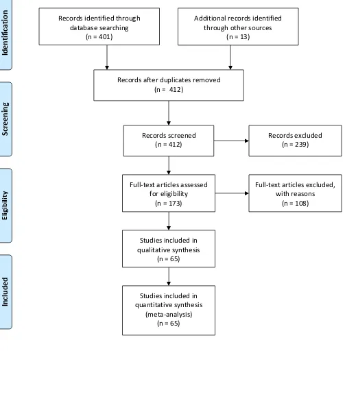
We collected published studies reporting psychophysical binocular summation ratios for luminance-defined stimuli at contrast detection threshold in observers with normal vision. These were obtained by searching PubMed using the term ‘binocular summation’ (401 hits on 19th January 2018) and then screening each study to determine its methodological details, yielding 52 studies. A further 13 relevant studies were included that were identified through secondary searches and the authors’ knowledge of the literature, giving a total of 65 studies (see Appendix 1 for a full PRISMA flow diagram). In some cases summation data were given in tables or in the text; in others they were estimated from published figures using computer software. In instances where data for a control and a clinical
group were reported, we included only the control data.
We performed the meta-analysis using estimates of summation ratios expressed in decibel (dB) units, defined as 20*log10(BSR), where BSR is the ratio of monocular to binocular thresholds expressed in Michelson contrast (or equivalently the ratio of binocular to monocular contrast sensitivity). In these units, a summation ratio of 2 is equivalent to 6dB, a ratio of 1 is equivalent to 0dB, and a ratio of Ö2 is equivalent to 3dB. Where possible, we calculated the mean for each observer across all experimental conditions (e.g. different spatial or temporal frequencies, depending on the study) and then computed a mean and standard deviation across observers, and used this to estimate 95% confidence intervals using the approximation ±1.96*SE. In other studies, data for individual observers were not available, and we estimated the standard deviation by pooling variances across conditions assuming negligible covariance between conditions (which is implausible, but gives an upper bound on the variance estimate). Where standard deviations (or standard errors) were given in linear units, we converted these to dB units before averaging. For some studies it was only possible to obtain the mean, and so a measure of variance is not given. The full meta-analysis summary table is included in Appendix 1.
2.2 Meta-analysis: results
This post-print version was created for open access dissemination through institutional repositories
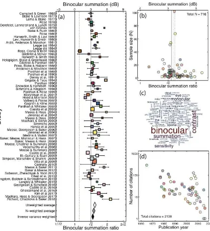
Figure 1: Meta-analysis summary. (a) Forest plot of binocular summation across 65 studies. Square symbol width is proportional to the log of the sample size plus one. Error bars give 95% confidence intervals, estimated using the approximation ±1.96*SE. The black vertical line gives the line of no effect, where binocular and monocular sensitivities are equal. The dashed vertical line gives an estimate of probability summation for two independently noisy signals. The grey vertical line gives the traditional value of Ö2. The white diamond gives the average across all studies (3.72dB, or a ratio of 1.53), weighting each study equally (ignoring sample size). The grey diamond gives the average weighted by the sample size of each study (3.54dB, or a ratio of 1.50). The black diamond gives the average weighted by the inverse variance of each study (3.35dB, or a ratio of 1.47). This latter estimate comprises only 55 studies, as a measure of variance was unavailable for 10 studies. The width of the diamonds spans the 95% confidence intervals. (b) Funnel plot showing sample size plotted against binocular summation for all 65 studies. The distribution of summation ratios is approximately symmetrical about the means (with the dotted, dashed and solid lines corresponding to the white, grey and black diamonds from panel (a)). (c) Word cloud showing the most frequent words used in the abstracts of
studies included in the meta-analysis. (d) Number of citations per article included (obtained from Web of Knowledge
on January 29th 2018), plotted against year of publication. Articles with no citations are omitted. Colours in panels (b,d)
This post-print version was created for open access dissemination through institutional repositories Much less clear from inspecting the individual
means is whether the population of studies shows summation above the classical value of Ö2. To determine this, we averaged across studies to produce aggregate estimates of summation. When each study is given equal weight (regardless of sample size), the mean level of summation was 1.53, as shown by the white diamond at the foot of Figure 1a. The lower bound of the 95% confidence interval was comfortably above the Ö2 level. We also calculated a weighted average, where each study was multiplied by its sample size, and the total divided by the sum of the weights (grey diamond in Figure 1a). This slightly reduced the mean summation ratio (to 1.50), but left the lower bound of the confidence interval above Ö2 (at 1.46). Finally, we weighted studies by the inverse of the variance across participants (black diamond in Figure 1a). An estimate of variance was available for 55 studies, with 5 of the remaining studies featuring only one participant, and the remaining 5 failing to report a useable measure of variability. Across these 55 studies, the weighted mean was 1.47, with the lower bound of the 95% confidence interval at 1.43. Therefore all three methods for weighting the summation ratios produced an average value that was significantly above the classical estimate of Ö2.
We next asked which methodological factors might lead to the inter-study variability in summation ratios. One methodological difference between studies is the way in which the unstimulated eye is treated during monocular conditions. In many studies (particularly older studies and those with a clinical focus) the unstimulated eye wore a patch, and was therefore completely dark during monocular conditions (N=13). Other studies use specialist equipment, such as stereoscopes, virtual reality headsets, or stereo shutter goggles to present mean luminance to the unstimulated eye on monocular trials (N=33). In these studies, trials from different conditions (binocular vs monocular presentation) can be interleaved so that the participant is unaware of whether one or both eyes are being stimulated on a given trial. It has been suggested that luminance from an otherwise unstimulated eye can have an effect on sensitivity to periodic stimuli presented to the other eye (Denny, Frumkes, Barris, & Eysteinsson, 1991; Yang & Stevenson, 1999), and this dichoptic ‘zero frequency’ masking might be
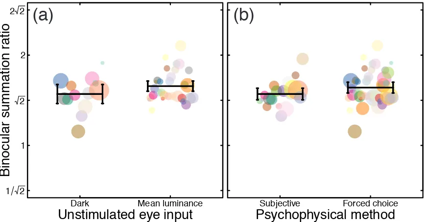
expected to influence binocular summation. Studies in which the unstimulated eye saw mean luminance on monocular trials reported slightly greater levels of binocular summation than studies involving patching (mean ratios of 1.57 vs 1.48, see Figure 2a). However, a Welch’s t-test comparing summation ratios from studies using these two methodologies (twelve studies in which the method was not clearly stated, and 7 studies using a translucent occluder were omitted) found that the difference was not significant (t=1.43, df=19.25, p=0.17).
A second difference across studies concerns the psychophysical methodology used to estimate thresholds. Many older studies used techniques such as the method of adjustment or yes/no tasks to estimate thresholds (N=19). These methods are subject to bias, from participants adjusting their criteria for setting thresholds (or for responding yes or no), which might be more severe in studies where the condition being tested (monocular or binocular) was made explicit by the use of a patch. More recent work (N=46) has tended to use bias-free forced-choice methods to avoid such problems. Bias-free methods produced slightly greater levels of summation (mean ratio 1.56) compared with other methods (mean ratio 1.48; see Figure 2b). Nevertheless, a Welch’s t-test found no significant difference between these two methodologies (t=1.70, df=40.96, p=0.10).
3 Summation varies with spatiotemporal stimulus properties
This post-print version was created for open access dissemination through institutional repositories
Figure 2: Effect of methodology on binocular summation. Panel (a) compares studies in which the unstimulated eye (in monocular conditions) viewed mean luminance, with studies in which it wore a patch and was therefore dark. Panel (b) compares studies that used criterion free forced-choice methods with studies that used other methods (such as the method of adjustment, or yes/no tasks). In both panels, data from a single study have a colour consistent with Figure 1a, and symbol diameter is proportional to the base-10 logarithm of sample size (plus an added constant to avoid sizes of zero for studies with only one participant). Black horizontal lines in give the unweighted means across studies, and error bars give 95% confidence intervals.
Previous studies have manipulated spatial (Campbell & Green, 1965; Ross, Clarke, & Bron, 1985; Simpson, Manahilov, & Shahani, 2009) and/or temporal (Baker & Meese, 2012; Rose, 1980) frequency experimentally, sometimes finding systematic effects on binocular summation. Yet we found no published study reporting summation as a function of both spatial and temporal frequency that manipulated both variables across a wide range. Such a study is necessary to validate the findings from the meta-analysis while controlling for potential methodological confounds (e.g. if spatiotemporal frequency covaried with stimulus size, psychophysical task, equipment used, or other factors such as mean luminance). Fortunately, archival data were available that met these requirements. Two experiments testing a wide range of different spatiotemporal conditions (termed set A and set B), were conducted at Aston University during 2004 and 2005. These data have previously been reported only in abstract form (Georgeson & Meese, 2007, 2005), but are presented here in full for the first time. Methodological details are available in Appendix 2.
3.1 Spatiotemporal study: results
Binocular summation was apparent in all conditions tested with both stimulus sets, with
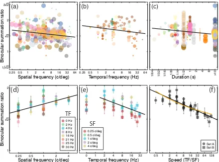
an overall average summation ratio of 1.65 (4.33dB). We plot the results in three ways in Figure 3d-f. Plotting binocular summation as a function of spatial frequency (collapsing across all temporal conditions) reveals an increase in summation with increasing spatial frequency (Figure 3d). The best fit regression line (in logarithmic units) had a highly significant positive slope of 0.05 (R2=0.40, t=5.25, p<0.001), meaning that an increase in spatial frequency of a factor of 10 will increase summation by around 12% (1dB). This effect is in the opposite direction to the effect of spatial frequency across the studies in the meta-analysis (see Figure 3a), which showed a slight negative effect of spatial frequency. We discuss possible explanations for this discrepancy in the next section.
There was a significant negative effect of temporal frequency (R2=0.33, t=-4.14, p<0.001) with a slope of -0.05 (excluding the static conditions which had a nominal frequency of 0 Hz). This suggests that a tenfold increase in temporal frequency will reduce summation by around 12% (see Figure 3e), broadly consistent with the estimate from the meta-analysis (a slope of -0.03, Figure 3b).
Dark Mean luminance
1 2
1 2 2 2 2
Unstimulated eye input
Bi
n
o
cu
la
r
su
mma
ti
o
n
r
a
ti
o
Subjective Forced choice
Psychophysical method
This post-print version was created for open access dissemination through institutional repositories
Figure 3: Effects of spatial and temporal stimulus properties on binocular summation. The upper row shows data from the meta-analysis, plotting summation as a function of spatial frequency (a), temporal frequency (b) and stimulus duration (c) using the same symbol size and colour conventions as in Figure 2. In (c), studies that allowed unlimited inspection time are assigned a duration of >10s. The lower row shows the results of two experiments measuring binocular summation as a function of spatial frequency (d), temporal frequency (e) and speed (f), given by the ratio of temporal frequency to spatial frequency, in deg/s. The same data are reproduced in each panel, except that the 0Hz data are omitted from panel (f). Error bars indicate ±1SE of the mean across observers (N=4 for each data point). Black lines in all panels are best fitting regression lines (on log-transformed values), and the orange curve in (f) is the
prediction of equation 2 when the exponent m depends on stimulus speed (see text for details).
Since summation increases with spatial frequency and decreases with temporal frequency, the data are consistent with an effect of implied stimulus speed. This measure, defined as the ratio of temporal to spatial frequency in deg/s, is a scalar quantity that has no implied direction. Replotted as a function of speed (Figure 3f), binocular summation shows a remarkably lawful decline, as indexed by the highly significant linear regression (R2=0.70, t=-8.7, p<0.001) with a slope of -0.05 in logarithmic units (black line). This holds across speeds varying over more than two orders of magnitude in the present experiment. Because summation depends on the strength of the exponent in equation 2, it follows that this exponent (m) can be considered a function of stimulus speed. Specifically, the function m = 1.14 + 0.28*log10(TF/SF), where TF is temporal frequency (in Hz) and SF is spatial frequency (in c/deg), provides the best least squares fit to the
data, as shown by the orange curve in Figure 3f. In short, increasing the early nonlinearity (m) with speed could account for the observed decrease in binocular summation.
3.2 Spatiotemporal study: discussion
The effect of temporal frequency on binocular summation is consistent between the meta-analysis and the experiment reported here. However higher spatial frequencies were associated with weaker summation in the meta-analysis, but stronger summation in the stand-alone experiment. What might account for this puzzling discrepancy?
One key factor that can act to depress empirical summation ratios is the sensitivity difference between the two eyes. In many studies, summation ratios are calculated by comparing binocular sensitivity with that of the more sensitive eye. When the two eyes are
0.25 0.5 1 2 4
1 2 2
Spatial frequency (c/deg)
Bi
n
o
cu
la
r
su
mma
ti
o
n
r
a
ti
o
0 Hz 2 Hz 4 Hz 8 Hz 16 Hz 21 Hz 25 Hz 30 Hz
0 1 2 4 8 16 32
Temporal frequency (Hz)
0.25 c/deg 0.5 c/deg 1 c/deg 2 c/deg 4 c/deg
0.5 1 2 4 8 16 32 64 128
Speed (TF/SF)
Set A Set B
(d)
(e)
(f )
TF
SF
1
/6
4
1
/3
2
1
/1
6
1
/8 1/4 1/2 1 2 4 8
>1
0
Duration (s)
0.25 0.5 1 2 4 8 16 32 64
Temporal frequency (Hz)
0.25 0.5 1 2 4 8 16 32 64
1 2 1 2 2 2 2
Spatial frequency (c/deg)
Bi
n
o
cu
la
r
su
mma
ti
o
n
r
a
ti
This post-print version was created for open access dissemination through institutional repositories approximately equal this should give an accurate
estimate of summation. However, as the sensitivity difference between the eyes increases, the ‘boost’ from the less sensitive eye becomes weaker. At low spatial frequencies, sensitivities are usually well balanced, but at higher frequencies optical and neural factors penalize the weaker eye and reduce its sensitivity (e.g. Pardhan, 1996). Therefore in the studies included in the meta-analysis, the apparent spatial frequency effect might in fact be due to monocular asymmetries in sensitivity. We next explore how differences in monocular sensitivity can influence estimates of binocular summation.
4 Individual differences in interocular sensitivity predict summation
Even individuals with intact binocular vision often exhibit asymmetries in sensitivity across the two eyes. For example, Pardhan (1996) measured binocular summation in older and younger participants at both 1 and 6c/deg. In the older group, interocular sensitivity ratios (worse eye/better eye) showed a greater imbalance at the higher spatial frequency (mean ratio 0.74) than at the lower frequency (mean ratio 0.85), and on a scatterplot of individual data points there was a strong relationship between the interocular sensitivity ratio and binocular summation. Such asymmetries will influence the levels of binocular summation measured experimentally, depending on precisely how summation is calculated.
By plotting summation for observers with naturally varying amounts of interocular sensitivity difference, we can measure the change in summation that occurs in individuals with large asymmetries, and also estimate the true level of neural binocular summation. We first do this by replotting data from a subset of 21 studies from the meta-analysis for which individual monocular thresholds for both eyes were available (total N=239). However because the diversity of stimulus conditions used across studies could influence the results (e.g. via the effects of spatiotemporal frequency reported above), we replicate our findings by collecting new data in a group of 41 observers using common stimulus conditions. Methodological details for this experiment, which was conducted at The University of York during 2017, are available in Appendix 3.
4.1 Results of individual differences analysis Binocular summation is plotted as a function of the threshold difference between the eyes in Figure 4. In the upper row the data are from a subset of 21 studies from the main meta-analysis, and in the lower row the data are from a single experiment. The monocular threshold difference was calculated by taking the absolute difference between left and right eye thresholds (in dB units). Binocular summation was calculated in two ways: first, by subtracting the binocular threshold from the lower of the two monocular thresholds (in dB units, plotted in panels 4a,c), and second, by subtracting the binocular threshold from the average of the two monocular thresholds (plotted in panels 4b,d).
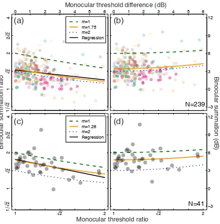
When summation is calculated relative to the best monocular threshold, there is a clear downward trend in both data sets, summarised by the significant negative correlations (Figure 4a, R=-0.19, p<0.01; Figure 4c, R=-0.43, p<0.01) and best fit linear regressions (black curves) with slopes of -0.28 (Figure 4a) and -0.5 (Figure 4c). The regression intercepts were 3.20dB (Figure 4a) and 4.89dB (Figure 4c). These intercepts imply binocular summation ratios of 1.45 (Figure 4a) and 1.76 (Figure 4c) when the eyes are equally sensitive. The slope of -0.5 (or -0.3) means that for every 1dB difference in sensitivity between the eyes, the measured level of binocular summation reduces by 0.5dB (or 0.3dB).
This post-print version was created for open access dissemination through institutional repositories
Figure 4: Change in binocular summation as a function of monocular sensitivity imbalance. In panels (a,c) summation is defined as the ratio of the binocular threshold and better of the two monocular thresholds. In panels (b,d) summation is defined as the ratio of the binocular threshold and the average of the two monocular thresholds. In all panels, a monocular threshold ratio of 1 indicates equal monocular sensitivities, and a ratio of 2 means that one eye was twice as sensitive as the other. Each data point represents one observer, either from studies in the meta-analysis with diverse spatiotemporal conditions (panel a,b; N=239), or from a stand-alone experiment with constant stimulus properties (panel c,d; N=41). The black curves in panel (a,c) are the best fitting regression line (using logarithmic values), with slopes of -0.3 (panel a) and -0.5 (panel c) and y-intercepts of 3.20dB (panel a) and 4.89dB (panel c). The remaining curves show summation predictions for a linear transducer (green dashed curves), square law transducer (blue dotted curves) and best fitting exponents (orange solid curves) under both calculation schemes.
Figure 4b,d replot the same data, but this time binocular summation was calculated relative to the average of the two monocular thresholds. Under this scheme, summation ratios are predicted to increase very slightly for larger monocular imbalances, because the higher monocular threshold in the weaker eye elevates the mean monocular threshold. This is borne out
by the very slight positive trend in the data points across both panels. Calculated in this way, the group average summation ratios were 3.56dB (a factor of 1.51, panel d) and 4.88dB (a factor of 1.75, panel d). The curves in Figure 4b,d show simulated summation levels for different transducer exponents as a function of interocular asymmetry (implemented in the model by
1 2 2
1
2
1
2
2
2
2
4
m=1 m=1.26 m=2 Regression
1 2 2
−3
0
3
6 9 12
N=41
Monocular threshold difference (dB)
Monocular threshold ratio
Bi
n
o
cu
la
r
su
mma
tio
n
(d
B)
Binocular vs best monocular Binocular vs mean monocular
0 1 2 3 4 5 6
1
2
1
2
2
2
2
4
m=1 m=1.75 m=2 Regression
0 1 2 3 4 5 6
−3
0
3
6 9 12
N=239
Bi
n
o
cu
la
r
su
mma
ti
o
n
ra
ti
o
(a)
(b)
This post-print version was created for open access dissemination through institutional repositories attenuating the input contrast to the weaker
eye). For a linear transducer (m=1, green dashed curve), a monocular difference of 6dB (a factor of 2) increases empirical summation by 0.5dB (around 6%). For a square law transducer (m=2, blue dotted curve), the expected increase is 1dB (12%). Again, the replotted data follow this trend qualitatively, and are well-described by the orange curve with exponents m=1.75 (panel b) and m=1.26 (panel d) that was fit to the data in Figure 4a,c.
By replotting a subset of the meta-analysis data and confirming with a new experiment, we demonstrated that individual differences in monocular sensitivity can affect empirically measured binocular summation. Overall, the data are consistent with monocular exponents of m=1.75 (a true binocular summation ratio of around 1.49) across studies with varying spatiotemporal properties (Figure 4a,c), and m=1.26 (a true binocular summation ratio of around 1.74) when methodological details are held constant (Figure b,d).
5 General Discussion
We revisited the extent to which contrast sensitivity improves for two eyes compared with one. Across a meta-analysis of 65 studies, and two additional experiments, we demonstrated conclusively that binocular summation is significantly greater than the traditional value of Ö2, and considered several factors that can affect empirical estimates of this parameter. Spatiotemporal frequency, and the sensitivity difference between the eyes both have an influence on empirical summation estimates. These effects suggest that there is no single canonical level of summation (as was originally proposed by Campbell & Green, 1965), but instead a range of values between approximately Ö2 and 2, depending on precise experimental conditions. We now discuss several of these factors in greater detail, and consider their importance for the clinical assessment of binocular function, and best practice for future studies.
5.1 Do higher spatial frequencies increase or decrease summation?
As demonstrated in Figure 4a,c, imbalances in monocular sensitivity can have a negative impact on binocular summation when it is calculated relative to the best monocular threshold. Since this is standard practice for many published studies (e.g. Chen et al., 2014; Longley & Whitaker, 2016; Pardhan & Rose, 1999), monocular asymmetries at higher spatial
frequencies are a plausible explanation for the apparent changes in binocular summation shown in Figure 3a. But in the spatiotemporal experiment, the raw monocular data were pooled to calculate a single threshold. Might this have led to spurious increases in summation at high spatial frequencies, as illustrated in Figure 4b,d? This is unlikely for two reasons. First, the effects are rather modest, even for quite large sensitivity differences (i.e. <1dB for a 6dB threshold difference). Second, monocular sensitivity differences of that magnitude would reduce the slope of the psychometric function used for estimating the pooled monocular threshold (because the pooled data would come from two underlying psychometric functions with a relative lateral displacement). The (geometric) mean slopes were almost identical across the binocular (mean Weibull b = 2.384) and monocular (mean Weibull b = 2.377) conditions, and showed no significant differences (p>0.05). We therefore conclude that the increase in summation at higher spatial frequencies is a genuine effect, but one that was previously obscured in published studies by methodological factors.
This post-print version was created for open access dissemination through institutional repositories 2007). Future clinical studies must therefore
exercise methodological diligence in using binocular summation to assess binocular function, especially in situations where monocular sensitivities may be unequal.
5.3 What is the best way to measure summation? Our results here point to some guidelines for how best to estimate neural binocular summation in future studies. Patching of the unstimulated eye should be avoided if at all possible, ideally by using equipment (stereoscopes, shutter goggles or virtual reality hardware) designed for binocular presentation. If this is not possible, then placing a frosted occluder in front of the unstimulated eye will ensure that it views an uncontoured field of nearly the same mean luminance. Unbiased forced-choice methods using adaptive staircases (or similar) are preferable to techniques in which the participant adjusts the stimulus contrast to reach some internal criterion (as this is subject to bias), or eye-chart-based methods (for which the set of possible thresholds is typically quantized to the range of stimuli on the chart).
Monocular thresholds should always be measured for each eye. If there are substantial differences in sensitivity across the eyes, then one option is to use a procedure in which the components of the binocular stimulus are normalized to the monocular detection thresholds (Baker et al., 2007). If this is not possible, then modelling the sensitivity difference can provide unbiased estimates of summation by calculating an attenuation weight for the weaker eye, finding the best exponent to describe the amount of summation measured, and inferring the level of summation that would be expected if sensitivities were equal (e.g. Figure 4a,c). For moderate sensitivity differences (e.g. <3dB), averaging the monocular thresholds is preferable to using the threshold of the better eye to calculate summation ratios, though this can slightly overestimate binocular summation (see Figure 4b,d).
5.4 Appropriate sample sizes for estimating binocular summation
The inverse variance weighted aggregate measure of binocular summation (given by the black diamond in Figure 1a) implies an effect size (Cohen’s d) of around 31 for detecting the existence of binocular summation (i.e. relative to a summation ratio of 1). This unusually large effect size means that even a study with only two participants should be capable of detecting the presence or absence of binocular summation (using a one-sample t-test) with 99.99% power.
When comparing binocular summation to the canonical value of Ö2, the effect size is still very large (d=3.22), meaning that a study with three participants has over 95% power. Our meta-analysis therefore demonstrates that the tradition of small sample sizes in psychophysical studies is often appropriate given the magnitude and stability of the effects involved, and the precision of the measurement techniques.
5.5 Summation for other visual cues
The present study was confined to the investigation of binocular summation of contrast at threshold using psychophysical techniques. Many of the studies we encountered while conducting the meta-analysis reported binocular summation for other visual tasks, including binocular summation for visual acuity, the detection of luminance at absolute threshold, and electroencephalographic (EEG) measures of binocular function. Understanding how the visual system integrates different cues across the eyes, and how the findings for contrast apply to different domains, will require further study. However, we note that the same general framework for signal combination and suppression that we discuss here and in our other work (Georgeson, Wallis, Meese, & Baker, 2016; Meese et al., 2006) has been successfully applied to understand binocular combination of cues such as motion (Maehara, Hess, & Georgeson, 2017) and contrast modulation (Georgeson & Schofield, 2016), as well as summation across space (Meese & Summers, 2007), time and orientation (Meese & Baker, 2013), and also to make accurate predictions regarding neural responses (Baker & Wade, 2017).
6 Conclusions
This post-print version was created for open access dissemination through institutional repositories
7 Acknowledgements
We are grateful to the participants in our experiments, and the authors of all the studies we included in our meta-analysis. Supported by EPSRC grants GR/S74515/01 and EP/H000038/1 awarded to TSM and MAG, and BBSRC grant BBH00159X1 awarded to MAG and TSM. Also supported in part by the Wellcome Trust (grant number 105624) through the Centre for Chronic Diseases and Disorders (C2D2) at the University of York.
8 Appendices
Appendix 1: Meta-analysis summary table and PRISMA diagram
Table A1: Meta-analysis summary table
Study N
BSR (dB)
SD (dB)
Citation
s Method Setup
Campbell & Green (1965) 2 2.966 0.310 289 MOA Occluder
Blake & Levinson (1977) 1 3.046 - 77 MOA Stereoscope
Lema & Blake (1977) 4 2.578 0.603 83 MOA Occluder
Rose (1978) 8 3.063 0.630 29 MOA Occluder
Derefeldt et al. (1979) 12 3.110 0.976 161 MOA Patch
von Grünau (1979) 1 5.480 - 0 2AFC Patch
Blake & Rush (1980) 3 3.174 0.199 10 MOA & 2AFC Stereoscope
Rose (1980) 6 3.964 1.222 11 MOA Occluder
Harwerth, Smith & Levi
(1980) 8 3.620 0.813 23 RT Patch/Diffuser
Levi, Harwerth & Smith
(1980) 1 3.111 - 41 2AFC Stereoscope
Arditi et al. (1981) 1 4.235 - 21 2AFC Stereoscope
Legge (1984a) 4 3.773 0.356 112 2AFC Stereoscope
Legge (1984b) 2 3.950 0.520 112 2AFC Stereoscope
Ross, Clarke & Bron (1985) 17 0.926 0.745 83 2AFC Patch
Gilchrist & McIver (1985) 2 2.608 1.524 21 MOA Not stated
Harwerth & Smith (1985) 3 4.660 1.340 14 MDL Not stated
Holopigian et al. (1986) 2 2.330 0.100 50 2AFC Stereoscope
Gilchrist & Pardhan (1987) 8 3.242 1.575 19 2AFC Not stated
Rose, Blake & Halpern (1988) 3 3.532 0.093 18 2AFC Stereoscope
Anderson & Movshon (1989) 4 3.342 1.015 49 MOA Stereoscope
Pardhan et al. (1989) 8 3.170 0.140 13 2AFC Stereoscope
Pardhan et al. (1990) 8 3.120 1.320 13 2AFC Stereoscope
Denny et al. (1991) 3 4.313 1.475 23 2AFC Stereoscope
Grigsby & Tsou (1994) 11 5.750 - 14 Yes/No Translucent patch
Pardhan (1996) 8 3.346 0.602 36 2AFC Patch
Snowden & Hammett (1996) 3 3.514 1.084 40 2AFC Goggles
Simmons & Kingdom (1998) 2 4.240 0.463 29 2AFC Goggles
Pardhan & Rose (1999) 4 3.340 1.511 8 2AFC Stereoscope
Marshman et al. (2001) 14 2.457 1.338 6 2AFC Occluder
Hood & Morrison (2002) 9 1.957 - 13 MAL Occluder
Valberg & Fosse (2002) 10 3.620 2.480 23 Yes/No Not stated
Gagnon & Kline (2003) 28 4.292 - 20 3AFC Patch
This post-print version was created for open access dissemination through institutional repositories
Cuesta et al. (2003) 54 3.280 - 25 3AFC Not stated
Meese & Hess (2004) 2 5.853 1.707 70 2AFC Stereoscope
Jiménez et al. (2004) 18 3.100 0.650 12 3AFC Not stated
Meese & Hess (2005) 2 5.120 1.354 28 2AFC Stereoscope
Maehara & Goryo (2005) 3 3.270 1.345 23 2AFC Stereoscope
Simmons (2005) 4 4.262 0.709 23 2AFC Stereoscope
Handa et al. (2005) 12 3.200 2.480 15 Eyechart Not stated
Meese et al. (2006) 5 4.550 0.795 128 2AFC Goggles
Jiménez et al. (2006) 68 3.743 9.291 27 Not stated Not stated
Medina & Mullen (2007) 3 4.429 1.726 5 2AFC Translucent patch
Baker et al. (2007) 3 3.279 0.839 95 2AFC Goggles
Baker, Meese & Hess (2008) 1 3.970 - 72 2AFC Goggles
Meese et al. (2008) 3 4.027 0.588 17 2AFC Goggles
Vedamurthy et al. (2008) 20 3.998 3.239 12 2AFC Goggles
Meese & Summers (2008) 3 5.030 0.808 40 2AFC Goggles
Castro et al. (2009) 28 2.415 0.517 13 Not stated Not stated
El-Gohary & Siam (2009) 15 4.155 2.640 0 Eyechart Not stated
Simpson et al. (2009) 51 3.192 2.969 7 2AFC Occluder
Villa et al. (2009)
10
2 3.660 - 3 Not stated Occluder
Connolly (2010) 12 3.464 4.222 10 Yes/No Opaque occluder
Meese & Baker (2011) 3 5.422 0.762 9 2AFC Goggles
Baker & Meese (2012) 9 3.264 1.592 2 2AFC Goggles
Sabesan et al. (2012) 5 2.704 1.260 6 2AFC Stereoscope
Chen et al. (2014) 22 2.582 1.853 4 2AFC Patch
Kingdom et al. (2015) 2 2.923 1.112 21 2AFC Stereoscope
Longley & Whitaker (2016) 2 4.130 0.110 1 2AFC Occluder (black)
Georgeson & Schofield (2016) 7 5.417 1.416 1 2AFC Goggles
Castro et al. (2016) 12 3.364 2.573 0 4AFC Not stated
Gheiratmand et al. (2016) 4 3.143 0.500 3 2AFC Stereoscope
Kim et al. (2017) 20 4.440 3.370 0 2AFC Patch
Maehara et al. (2017) 3 4.990 0.290 0 2AFC Stereoscope
Richard et al. (2018) 8 6.630 2.231 0 2AFC Goggles
This post-print version was created for open access dissemination through institutional repositories Figure A1: PRISMA flow diagram
Records identified through database searching
(n = 401)
S
cr
e
e
n
in
g
In
cl
u
d
e
d
E
li
g
ib
il
it
y
Id
e
n
ti
fi
ca
ti
o
n
Additional records identified through other sources
(n = 13)
Records after duplicates removed (n = 412)
Records screened (n = 412)
Records excluded (n = 239)
Full-text articles assessed for eligibility
(n = 173)
Full-text articles excluded, with reasons
(n = 108)
Studies included in qualitative synthesis
(n = 65)
Studies included in quantitative synthesis
This post-print version was created for open access dissemination through institutional repositories
Appendix 2: Spatiotemporal experiment: methods Target stimuli were horizontal sine-wave gratings with spatial frequencies of 0.25, 0.5, 1, 2 and 4c/deg (set A), or 0.25 and 1c/deg (set B). Stimulus contrast was spatially windowed by a circular aperture with smoothed edges and a diameter at half-height of 4 degrees. Stimulus contrast was temporally windowed by one cycle of a raised cosine (duration 500 ms) and within that envelope contrast flickered sinusoidally in counterphase at frequencies of 2, 4, 8 and 16Hz (set A) or 2, 4, 8, 16, 21, 25 and 30Hz (set B). There was also a static condition, in which the stimulus did not flicker (i.e. a nominal frequency of 0Hz). All factorial combinations of spatial and temporal frequencies within a set were tested. The experiments were completed by independent groups of naïve observers for set A (N=4) and set B (N=4). All observers had no reported history of binocular abnormalities, and wore their prescribed optical correction if required.
Stimuli were generated using a Bits++ video interface (Cambridge Research Systems Ltd., Kent, UK) controlled by an Apple Macintosh computer running Matlab, and presented with 14-bit luminance resolution on a gamma-corrected Clinton Monoray monitor running at 150Hz. The display was viewed through ferro-electric FE1 stereo shutter goggles synchronized with the monitor refresh rate to permit independent control of images to the left and right eyes via frame interleaving. Mean luminance, as seen through the alternating goggles, was 26 cd/m2. The goggles ensured that during monocular conditions, the unstimulated eye viewed mean luminance.
Stimuli were presented for 500ms in one of two intervals, each marked by a beep, with a gap of 500ms between intervals. In one interval the target was presented, with its contrast determined by a 3-down 1-up staircase algorithm. The other interval was blank. Any given trial could either be monocular (left or right eye) or binocular, and the observer was not informed of this. Stimuli were blocked by spatiotemporal condition. Observers indicated which interval contained the target using a keypad and received auditory feedback regarding accuracy. Staircase algorithms terminated after 100 trials, and each observer repeated the experiment four times, resulting in 20,000 (set A) or 12,800 (set B) trials per observer (in set B there were additional trials in which the stimuli were in antiphase across the eyes, but these data are not reported here). Thresholds for individual observers were
estimated by fitting Weibull functions to the psychometric data pooled across all repetitions, and taking the contrast at the 81.6% correct point. Binocular summation was calculated as the difference (in dB units) between monocular and binocular thresholds.
Appendix 3: Individual differences experiment: methods
Target stimuli were horizontal sine-wave gratings with a spatial frequency of 1c/deg, windowed by a circular aperture with its edges smoothed by a cosine function to a diameter of 5 degrees. They were generated using a ViSaGe stimulus generator (Cambridge Research Systems Ltd., Kent, UK) controlled by a PC running Matlab, and presented with 14-bit luminance resolution on a gamma-corrected Clinton Monoray monitor running at 120Hz. The display was viewed through ferro-electric stereo shutter goggles synchronized with the monitor refresh rate to permit independent control of images to the left and right eyes via frame interleaving. The goggles ensured that during monocular conditions, the unstimulated eye viewed mean luminance.
This post-print version was created for open access dissemination through institutional repositories negative or extremely shallow slopes,
implausibly high or low thresholds (exceeding ±3SD of the group mean), or could not be fitted satisfactorily. The final data set consisted of 41 observers whose results met these criteria for all three ocularity conditions.
9 References
Anderson, P. A., & Movshon, J. A. (1989). Binocular
combination of contrast signals. Vision Research,
29(9), 1115–1132.
Arditi, A. R., Anderson, P. A., & Movshon, J. A. (1981). Monocular and binocular detection of moving
sinusoidal gratings. Vision Research, 21(3), 329–
336.
Baker, D. H., & Graf, E. W. (2009). On the relation between dichoptic masking and binocular rivalry.
Vision Research, 49(4), 451–459.
https://doi.org/10.1016/j.visres.2008.12.002 Baker, D. H., & Meese, T. S. (2012). Interocular transfer
of spatial adaptation is weak at low spatial
frequencies. Vision Research, 63, 81–87.
https://doi.org/10.1016/j.visres.2012.05.002 Baker, D. H., Meese, T. S., & Hess, R. F. (2008). Contrast
masking in strabismic amblyopia: attenuation, noise, interocular suppression and binocular
summation. Vision Research, 48(15), 1625–1640.
https://doi.org/10.1016/j.visres.2008.04.017 Baker, D. H., Meese, T. S., Mansouri, B., & Hess, R. F.
(2007). Binocular summation of contrast remains
intact in strabismic amblyopia. Investigative
Ophthalmology & Visual Science, 48(11), 5332–
5338. https://doi.org/10.1167/iovs.07-0194 Baker, D. H., & Wade, A. R. (2017). Evidence for an
Optimal Algorithm Underlying Signal Combination
in Human Visual Cortex. Cerebral Cortex, 27, 254–
264. https://doi.org/10.1093/cercor/bhw395 Baker, D. H., Wallis, S. A., Georgeson, M. A., & Meese, T.
S. (2012). Nonlinearities in the binocular
combination of luminance and contrast. Vision
Research, 56, 1–9.
https://doi.org/10.1016/j.visres.2012.01.008 Blake, R., & Levinson, E. (1977). Spatial properties of
binocular neurones in the human visual system.
Experimental Brain Research, 27(2), 221–232.
Blake, R., & Rush, C. (1980). Temporal properties of binocular mechanisms in the human visual system.
Experimental Brain Research, 38(3), 333–340.
Campbell, F. W., & Green, D. G. (1965). Monocular
versus binocular visual acuity. Nature, 208(5006),
191–192.
Castro, J. J., Jiménez, J. R., Hita, E., & Ortiz, C. (2009). Influence of interocular differences in the Strehl
ratio on binocular summation. Ophthalmic &
Physiological Optics: The Journal of the British
College of Ophthalmic Opticians (Optometrists),
29(3), 370–374.
https://doi.org/10.1111/j.1475-1313.2009.00643.x
Castro, J. J., Soler, M., Ortiz, C., Jiménez, J. R., & Anera, R. G. (2016). Binocular summation and visual function with induced anisocoria and monovision.
Biomedical Optics Express, 7(10), 4250–4262.
https://doi.org/10.1364/BOE.7.004250
Chen, Z., Li, J., Thompson, B., Deng, D., Yuan, J., Chan, L., … Yu, M. (2014). The effect of Bangerter filters on binocular function in observers with amblyopia.
Investigative Ophthalmology & Visual Science,
56(1), 139–149.
https://doi.org/10.1167/iovs.14-15224
Connolly, D. M. (2010). Spatial contrast sensitivity at
twilight: luminance, monocularity, and
oxygenation. Aviation, Space, and Environmental
Medicine, 81(5), 475–483.
Cuesta, J. R. J., Anera, R. G., Jiménez, R., & Salas, C. (2003). Impact of interocular differences in corneal asphericity on binocular summation.
American Journal of Ophthalmology, 135(3), 279–
284.
Denny, N., Frumkes, T. E., Barris, M. C., & Eysteinsson, T. (1991). Tonic interocular suppression and
binocular summation in human vision. The Journal
of Physiology, 437, 449–460.
Derefeldt, G., Lennerstrand, G., & Lundh, B. (1979). Age variations in normal human contrast sensitivity.
Acta Ophthalmologica, 57(4), 679–690.
El-Gohary, A. A., & Siam, G. A. (2009). Stereopsis and Contrast Sensitivity Binocular Summation in Early
Glaucoma. Research Journal of Medicine and
Medical Sciences, 4(1), 85–88.
Gagnon, R. W. C., & Kline, D. W. (2003). Senescent effects on binocular summation for contrast
sensitivity and spatial interval acuity. Current Eye
Research, 27(5), 315–321.
Georgeson, M.A., Meese, T.S., 2007. Binocular combination at threshold: temporal filtering and summation of signals in separate ON and OFF channels. Perception 36(S), 60.
Georgeson, M.A., Meese, T.S., 2005. Binocular summation at contrast threshold: a new look. Perception 34(S), 138.
Georgeson, M. A., & Schofield, A. J. (2016). Binocular functional architecture for detection of
contrast-modulated gratings. Vision Research, 128, 68–82.
https://doi.org/10.1016/j.visres.2016.09.005 Georgeson, M. A., Wallis, S. A., Meese, T. S., & Baker, D.
H. (2016). Contrast and lustre: A model that accounts for eleven different forms of contrast
discrimination in binocular vision. Vision Research,
129, 98–118.
https://doi.org/10.1016/j.visres.2016.08.001 Gheiratmand, M., Cherniawsky, A. S., & Mullen, K. T.
(2016). Orientation tuning of binocular
summation: a comparison of colour to achromatic
contrast. Scientific Reports, 6, 25692.
https://doi.org/10.1038/srep25692
Gilchrist, J., & McIver, C. (1985). Fechner’s paradox in
binocular contrast sensitivity. Vision Research,
25(4), 609–613.
Gilchrist, J., & Pardhan, S. (1987). Binocular contrast detection with unequal monocular illuminance.
Ophthalmic & Physiological Optics: The Journal of the British College of Ophthalmic Opticians
(Optometrists), 7(4), 373–377.
Grigsby, S. S., & Tsou, B. H. (1994). Grating and flicker sensitivity in the near and far periphery: naso-temporal asymmetries and binocular summation.
Vision Research, 34(21), 2841–2848.
This post-print version was created for open access dissemination through institutional repositories binocular summation after monocular reading
adds. Journal of Cataract and Refractive Surgery,
31(8), 1588–1592.
https://doi.org/10.1016/j.jcrs.2005.01.015 Harwerth, R. S., & Smith, E. L. (1985). Binocular
summation in man and monkey. American Journal
of Optometry and Physiological Optics, 62(7), 439–
446.
Harwerth, R. S., Smith, E. L., & Levi, D. M. (1980). Suprathreshold binocular interactions for grating
patterns. Perception & Psychophysics, 27(1), 43–50.
https://doi.org/10.3758/BF03199905
Hess, R. F., & Howell, E. R. (1977). The threshold contrast sensitivity function in strabismic amblyopia: evidence for a two type classification.
Vision Research, 17(9), 1049–1055.
Holopigian, K., Blake, R., & Greenwald, M. J. (1986).
Selective losses in binocular vision in
anisometropic amblyopes. Vision Research, 26(4),
621–630.
Hood, A. S., & Morrison, J. D. (2002). The dependence of binocular contrast sensitivities on binocular single vision in normal and amblyopic human
subjects. The Journal of Physiology, 540(Pt 2), 607–
622.
Jiménez, J. R., Ponce, A., & Anera, R. G. (2004). Induced
aniseikonia diminishes binocular contrast
sensitivity and binocular summation. Optometry
and Vision Science: Official Publication of the
American Academy of Optometry, 81(7), 559–562.
Jiménez, J. R., Villa, C., Anera, R. G., Gutiérrez, R., & del Barco, L. J. (2006). Binocular visual performance
after LASIK. Journal of Refractive Surgery
(Thorofare, N.J.: 1995), 22(7), 679–688.
Kim, Y. J., Reynaud, A., Hess, R. F., & Mullen, K. T. (2017). A Normative Data Set for the Clinical Assessment of Achromatic and Chromatic Contrast
Sensitivity Using a qCSF Approach. Investigative
Ophthalmology & Visual Science, 58(9), 3628–3636.
https://doi.org/10.1167/iovs.17-21645
Kingdom, F. A. A., Baldwin, A. S., & Schmidtmann, G. (2015). Modeling probability and additive
summation for detection across multiple
mechanisms under the assumptions of signal
detection theory. Journal of Vision, 15(5), 1.
https://doi.org/10.1167/15.5.1
Legge, G. E. (1984a). Binocular contrast summation--I.
Detection and discrimination. Vision Research,
24(4), 373–383.
Legge, G. E. (1984b). Binocular contrast
summation--II. Quadratic summation. Vision Research, 24(4),
385–394.
Lema, S. A., & Blake, R. (1977). Binocular summation in
normal and stereoblind humans. Vision Research,
17(6), 691–695.
Levi, D. M., Harwerth, R. S., & Smith, E. L. (1980). Binocular interactions in normal and anomalous
binocular vision. Documenta Ophthalmologica.
Advances in Ophthalmology, 49(2), 303–324.
Longley, C., & Whitaker, D. (2016). Google Glass Glare: disability glare produced by a head-mounted
visual display. Ophthalmic & Physiological Optics:
The Journal of the British College of Ophthalmic
Opticians (Optometrists), 36(2), 167–173.
https://doi.org/10.1111/opo.12264
Maehara, G., & Goryo, K. (2005). Binocular, Monocular
and Dichoptic Pattern Masking. Optical Review,
12(2), 76–82.
https://doi.org/10.1007/PL00021542
Maehara, G., Hess, R. F., & Georgeson, M. A. (2017). Direction discrimination thresholds in binocular, monocular, and dichoptic viewing: Motion
opponency and contrast gain control. Journal of
Vision, 17(1), 7. https://doi.org/10.1167/17.1.7
Marshman, W. E., Dawson, E., Neveu, M. M., Morgan, M. J., & Sloper, J. J. (2001). Increased binocular enhancement of contrast sensitivity and reduced
stereoacuity in Duane syndrome. Investigative
Ophthalmology & Visual Science, 42(12), 2821–
2825.
Medina, J. M., & Mullen, K. T. (2007). Colour-luminance
interactions in binocular summation. Vision
Research, 47(8), 1120–1128.
https://doi.org/10.1016/j.visres.2007.01.015 Meese, T. S., & Baker, D. H. (2011). A reevaluation of
achromatic spatio-temporal vision: Nonoriented filters are monocular, they adapt, and can be used
for decision making at high flicker speeds.
I-Perception, 2(2), 159–182.
https://doi.org/10.1068/i0416
Meese, T. S., & Baker, D. H. (2013). A Common Rule for Integration and Suppression of Luminance
Contrast across Eyes, Space, Time, and Pattern.
I-Perception, 4(1), 1–16.
https://doi.org/10.1068/i0556
Meese, T. S., Challinor, K. L., & Summers, R. J. (2008). A common contrast pooling rule for suppression
within and between the eyes. Visual Neuroscience,
25(4), 585–601.
https://doi.org/10.1017/S095252380808070X Meese, T. S., Georgeson, M. A., & Baker, D. H. (2006).
Binocular contrast vision at and above threshold.
Journal of Vision, 6(11), 7–7.
https://doi.org/10.1167/6.11.7
Meese, T. S., & Hess, R. F. (2004). Low spatial frequencies are suppressively masked across spatial scale, orientation, field position, and eye of
origin. Journal of Vision, 4(10), 843–859.
https://doi.org/10.1167/4.10.2
Meese, T. S., & Hess, R. F. (2005). Interocular suppression is gated by interocular feature
matching. Vision Research, 45(1), 9–15.
https://doi.org/10.1016/j.visres.2004.08.004 Meese, T. S., & Summers, R. J. (2007). Area summation
in human vision at and above detection threshold.
Proceedings. Biological Sciences, 274(1627), 2891–
2900. https://doi.org/10.1098/rspb.2007.0957 Meese, T. S., & Summers, R. J. (2012). Theory and data
for area summation of contrast with and without
uncertainty: Evidence for a noisy energy model. J
Vis, 12, (11): 9.
Pardhan, S. (1996). A comparison of binocular
summation in young and older patients. Current
Eye Research, 15(3), 315–319.
Pardhan, S., & Gilchrist, J. (1992). Binocular contrast summation and inhibition in amblyopia. The influence of the interocular difference on binocular
contrast sensitivity. Documenta Ophthalmologica.
Advances in Ophthalmology, 82(3), 239–248.
This post-print version was created for open access dissemination through institutional repositories
inhibition. Ophthalmic & Physiological Optics: The
Journal of the British College of Ophthalmic
Opticians (Optometrists), 9(1), 46–49.
Pardhan, S., Gilchrist, J., Douthwaite, W., & Yap, M. (1990). Binocular inhibition: psychophysical and
electrophysiological evidence. Optometry and
Vision Science: Official Publication of the American
Academy of Optometry, 67(9), 688–691.
Pardhan, S., & Rose, D. (1999). Binocular and monocular detection of Gabor patches in binocular
two-dimensional noise. Perception, 28(2), 203–
215. https://doi.org/10.1068/p2739
Pardhan, S., & Whitaker, A. (2003). Binocular summation to gratings in the peripheral field in older subjects is spatial frequency dependent.
Current Eye Research, 26(5), 297–302.
Richard, B., Chadnova, E., & Baker, D. H. (2018). Binocular vision adaptively suppresses delayed
monocular signals. Neuroimage, 172: 753-765.
Rose, D. (1978). Monocular versus binocular contrast
thresholds for movement and pattern. Perception,
7(2), 195–200. https://doi.org/10.1068/p070195
Rose, D. (1980). The binocular: monocular sensitivity ratio for movement detection varies with temporal
frequency. Perception, 9(5), 577–580.
https://doi.org/10.1068/p090577
Rose, D., Blake, R., & Halpern, D. L. (1988). Disparity
range for binocular summation. Investigative
Ophthalmology & Visual Science, 29(2), 283–290.
Ross, J. E., Clarke, D. D., & Bron, A. J. (1985). Effect of age on contrast sensitivity function: uniocular and
binocular findings. The British Journal of
Ophthalmology, 69(1), 51–56.
Sabesan, R., Zheleznyak, L., & Yoon, G. (2012). Binocular visual performance and summation after
correcting higher order aberrations. Biomedical
Optics Express, 3(12), 3176–3189.
https://doi.org/10.1364/BOE.3.003176
Shaw, W. A., Newman, E. B., & Hirsh, I. J. (1947). The difference between monaural and binaural
thresholds. Journal of Experimental Psychology,
37(3), 229–242.
Simmons, D. R. (2005). The binocular combination of
chromatic contrast. Perception, 34(8), 1035–1042.
https://doi.org/10.1068/p5279
Simmons, D. R., & Kingdom, F. A. (1998). On the
binocular summation of chromatic contrast. Vision
Research, 38(8), 1063–1071.
Simpson, W. A., Manahilov, V., & Shahani, U. (2009).
Two eyes: square root 2 better than one? Acta
Psychologica, 131(2), 93–98.
https://doi.org/10.1016/j.actpsy.2009.03.006 Snowden, R. J., & Hammett, S. T. (1996). Spatial
frequency adaptation: threshold elevation and
perceived contrast. Vision Research, 36(12), 1797–
1809.
Tyler, C. W., & Chen, C. C. (2000). Signal detection theory in the 2AFC paradigm: attention, channel
uncertainty and probability summation. Vision
Research, 40(22), 3121–3144.
Valberg, A., & Fosse, P. (2002). Binocular contrast inhibition in subjects with age-related macular
degeneration. Journal of the Optical Society of
America. A, Optics, Image Science, and Vision, 19(1),
223–228.
Vedamurthy, I., Suttle, C. M., Alexander, J., & Asper, L. J. (2008). A psychophysical study of human binocular interactions in normal and amblyopic
visual systems. Vision Research, 48(14), 1522–
1531.
https://doi.org/10.1016/j.visres.2008.04.004 Villa, C., Jiménez, J. R., Anera, R. G., Gutiérrez, R., & Hita,
E. (2009). Visual performance after LASIK for a Q-optimized and a standard ablation algorithm.
Applied Optics, 48(30), 5741–5747.
von Grünau, M. (1979). Binocular summation and the
binocularity of cat visual cortex. Vision Research,
19(7), 813–816.
Yang, J., & Stevenson, S. B. (1999). Post-retinal
processing of background luminance. Vision