An efficient quantum compiler that reduces T count

White Rose Research Online URL for this paper:

http://eprints.whiterose.ac.uk/136466/

Version: Accepted Version

Article:

Campbell, E. and Heyfron, L. (2018) An efficient quantum compiler that reduces T count.

Quantum Science and Technology, 4 (1). 015004. ISSN 2058-9565

https://doi.org/10.1088/2058-9565/aad604

© 2018 IOP Publishing Ltd. This is an author produced version of a paper subsequently

published in Quantum Science and Technology. Article available under the terms of the

CC-BY-NC-ND licence (https://creativecommons.org/licenses/by-nc-nd/3.0/).

[email protected] https://eprints.whiterose.ac.uk/

Reuse

This article is distributed under the terms of the Creative Commons Attribution-NonCommercial-NoDerivs (CC BY-NC-ND) licence. This licence only allows you to download this work and share it with others as long as you credit the authors, but you can’t change the article in any way or use it commercially. More

information and the full terms of the licence here: https://creativecommons.org/licenses/

Takedown

If you consider content in White Rose Research Online to be in breach of UK law, please notify us by

Luke E. Heyfron1,∗ _{and Earl T. Campbell}1,†

1_{Department of Physics and Astronomy, University of Sheffield, Sheffield, UK}

(Dated: 25th _{May 2018)}

Before executing a quantum algorithm, one must first decompose the algorithm into machine-level instructions compatible with the architecture of the quantum computer, a process known as quantum compiling. There are many different quantum circuit decompositions for the same algorithm but it is desirable to compile leaner circuits. A fundamentally important cost metric is theT _{count – the}

number ofT gates in a circuit. For the single qubit case, optimal compiling is essentially a solved problem. However, multi-qubit compiling is a harder problem with optimal algorithms requiring classical runtime exponential in the number of qubits. Here, we present and compare several efficient quantum compilers for multi-qubit Clifford +T circuits. We implemented our compilers in C++ and benchmarked them on random circuits, from which we determine that our TODD compiler yields the lowestT _{counts on average. We also benchmarked TODD on a library of reversible logic}

circuits that appear in quantum algorithms and found that it reduced theT count for 97% of the circuits with an average T-count saving of 20% when compared against the best of all previous circuit decompositions.

Compiling is the conversion of an algorithm into a series of hardware level commands or elementary gates. Better compilers can implement the same algorithm using fewer hardware level instructions, reducing runtime and other resources. Quantum compiling or gate-synthesis is the analogous task for a quantum computer and is especially important given the current expense of quantum hardware. Early in the field, Solovay and Kitaev proposed a general purpose compiler for any universal set of elementary gates [1–3]. Newer compilers exploit the specific structure of the Clifford+T gate set and have reduced quantum circuit depths by several orders of magnitude [4–7], often improving the classical compile time. The Clifford+T gate set is natural since it is the fault-tolerant logical gate set in almost every computing architecture [8]. Moreover, fault-tolerance protocols have been proposed such as magic state distillation [9] that lead to a cost per T

gate which is several hundred times larger than that of Clifford gates [10–12], which suggestsT count as the key metric of compiler performance. Furthermore, the T count is an important metric beyond the standard compiling problem because it relates to the classical overhead of simulating quantum circuits [16, 40, 41] as well as the distillation cost of synthillation [24]. For these reasons, it is clear that developing methods for minimizing theT count is crucial for a variety of applications in quantum computation.

Significant progress has been made on synthesis of single-qubit unitaries from Clifford+T gates. For purely unitary synthesis, the problem is essentially solved since we have a compiler that is asymptotically optimal and efficient [4, 7]. Although further improvements are possible beyond unitary circuits, by making use of ancilla qubits and measurements [13– 16] or adding an element of randomness to compiling [17, 18]. On the other hand, the multi-qubit problem is much more challenging. An algorithm for multi-qubit unitary synthesis over the Clifford+T gate set is known that is provably optimal in terms of theT count but the compile runtime is exponential in the number of qubits [6, 19]. Compilers with efficient runtimes have been proposed but with no promise ofT count optimality [20, 21]. We seek a compiler that runs efficiently and yields circuits withT counts that are as low as practically achievable.

A useful strategy is to take an initial Clifford+T circuit and split it into subcircuits containing Hadamards and subcircuits containing CNOT, S and T gates. One can then attempt to reduce the number ofT gates within just the latter type of subcircuit. Amy and Mosca recently showed that this restricted problem is formally equivalent to error decoding on a class of Reed-Muller codes [22], which is in turn equivalent to finding the symmetric tensor rank of a 3-tensor [23]. Unfortunately, even this easier sub-problem is difficult to solve optimally. Nevertheless, it is more amenable to efficient solvers that offer reductions inT count. Amy and Mosca proved that ann-qubit subcircuit (containing CNOT, S and

T gates) has an optimal decomposition into n2_{/2 +O(n) T gates. At the time, known efficient compilers could only}

promise an output circuit with no more than O(n3_{) T gates. Later, Campbell and Howard [24] sketched a compiler}

that is efficient and promises an output circuit with at most n2_{/2 +O(n) T gates. This shows efficient compilers can}

in this sense be “near-optimal” with respect to worst case scaling. On the mathematical level, Campbell and Howard exploited a previously known efficient and optimal solver for a related 2-tensor problem [25] but suitably modified so that it nearly-optimally solves the required 3-tensor problem.

This paper develops several different compilers that have polynomial runtime innand are near-optimal in the above sense when restricted to CNOT+T circuits. We modify the compiler to also accommodate Hadamard gates using a gadgetisation trick that requires additional resources (measurements, feed-forward and ancillas) and find that it performs well in practice. We provide the first implementations of such compilers (the source code is available here [44]) and compare performance against: a family of random circuits; and a library of benchmark circuits that implement actual quantum algorithms. For random circuits, we observeO(n2_{) scaling inT count for all variants of our compiling approach}

∗_{[email protected]} †_{[email protected]}

compared withO(n3) scaling for compilers based on earlier work. Quantum algorithms are highly structured and far from random, so the number ofT gates can not be meaningfully compared with the worst case scaling. Instead, we benchmark against the best previously known results and found on average a 20%T count reduction. In one instance, our compiler gave a 51%T count reduction and it performed better than previous results for all but one of the benchmarked circuits. Of course, theT count is not the only metric relevant to gate synthesis. We discuss the limitations of theT count, as well as other metrics in section IV C.

All of the near-optimal compilers described in this paper look for inspiration in algorithms for the related 2-tensor problem, which we call Lempel’s algorithm. We give specific details for a compiler here called TOOL (Target Optimal by Order Lowering) that comes in two different flavours (with and without feedback). The TOOL compilers can be considered concrete versions of the approach outlined by Campbell and Howard [24]. Also described in this paper is the TODD (Third Order Duplicate and Destroy) compiler, which is again inspired by Lempel but in a more direct and elegant way than TOOL. In benchmarking, we find that TODD often achieved even lowerT count than TOOL.

I. PRELIMINARIES

The Pauli group onnqubits Pn _{is the set of alln-fold tensor products of the single qubit Pauli operators{X, Y, Z,I}}

with allowed coefficients∈ {±1,±i}. Thekth _{level of theClifford hierarchy C}n

k is defined as follows,

Cn

k ={U |UPnU †_{⊆ C}n

k−1}, (1)

with recursion terminated byCn

1 =Pn. The Clifford group onnqubits Cn is the normalizer ofPn. We defineDkn to be

the diagonal elements ofhCN OT, Ti. We will omit the superscriptnwhen the number of qubits is obvious from context. We define Clifford to be any generating set for the Clifford group on n qubits such as {CN OT, H, S}. We define the CNOT + T gate set to be{CNOT, S, T}, where we include the phase gateS =T2 _{as a separate gate due to the magic}

states cost model for gate synthesis [9]. A quantum circuit decomposition for a unitary U is denoted U; conversely we say thatU implements U. Similarly, a circuitE implements non-unitary channel ρ→ε(ρ). We refer to a circuit U that implements aU ∈ D3 as adiagonal CNOT +T circuit.

5

Convert back to circuit INPUT: matrix

OUTPUT: circuit implementing using T-gates

A

U

m

T-optimiser

INPUT: symmetric tensor OUTPUT: low rank decomposition

S

Extract Signature INPUT: phase gate

S

Uf= x

ωf(x)_{|x x|}

OUTPUT: symmetric tensor

Sα,β,γ= m

j=1

Aα,jAβ,jAγ,j

T

T T T

T S T T T S T H H H H H S T T

S H T

T Clifford+ circuit T 1 4 6 T T T T S T T S T T T T S CNOT+ circuit T Cl iff or d C1

{

|+⊗h

X X Cl iff or d C2 · ·· X Cl iff or d Ch · · · 2 x r eg is ter y r eg is ter CNOT circuit Uf non-Cl iff or

d phase g

a

te

{

|+⊗h

Cl iff or d C1 X X Cl iff or d C2 · ·· X Cl iff or d Ch · · · 3 _U E

U

V

II. WORK-FLOW OVERVIEW

In this section, we give a high level work-flow of our approach to compiling as sketched in Fig. 1. In stages 1-3, some simple circuit preprocessing is performed so that a Clifford+T circuit is converted into a form where the only non-Clifford part is a diagonal CNOT+T gate (an element of D3). Subsection II A describes this preprocessing. In stages 4-6, the

technically difficult aspect of compiling is addressed using a series of different algebraic representations of the circuit and these stages are described in Subsection II B.

A. Circuit preprocessing

The input circuitUin ∈ hClifford, Tiimplements some unitaryU. It acts on a register we denote x, which is composed

ofnqubits and spans the Hilbert spaceHx. The output of our compiler is a circuitEoutcomposed of Clifford andT gates

but additionally allows: the preparation of|+istates; measurement in the Pauli-X basis, and classical feedforward. To account for ancilla|+iqubits, we include a register labelled y that is composed of hqubits and spans the Hilbert space

Hy. The circuitEout will realise the input unitary after the y register is traced out

Try[εout(ρx)] = Try[εpost(V(ρx⊗ |+i h+|⊗h))V†)], (2)

=U ρxU†, (3)

whereρxis the density matrix for an arbitrary input pure state onHx. Furthermore,V ∈ C3is the unitary portion ofEout,

andεpost is a quantum channel that is associated with the sequence of Pauli-X measurements and subsequent classically

controlled Clifford gates,C1, C2, . . . , Ch, seen in Fig. 1.

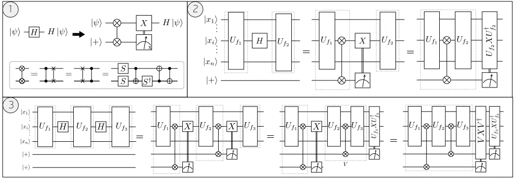
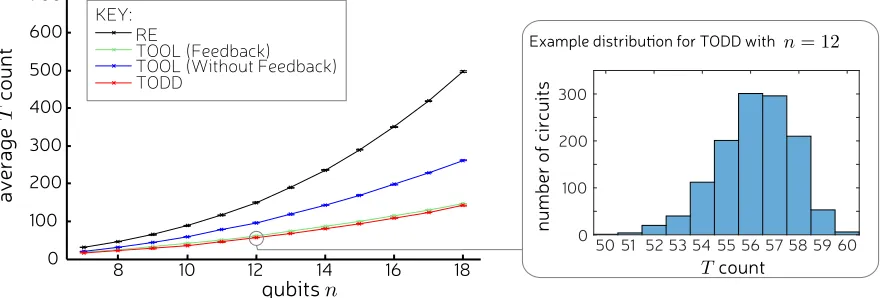
We emphasize that later stages of compiling will make use of a framework valid only for CNOT +T circuits, which makes Hadamard gates an obstacle. There are two commonly used methods for dealing with Hadamard gates: first, we can partition the quantum circuit into alternatinghCN OT, TiandhHisubcircuits and optimize each CNOT + T subcircuit independently [20]. The second way is to replace each Hadamard gate with a gadget (see for example references [26, 27]) that makes use of extra resources (ancillas, measurements and feedforward). The central portion of the gadget contains all of the non-Clifford behaviour and is in the CNOT + T gate set, so is directly compatible with ourT-optimizers. The remainder of this section focusses on the second method (Hadamard gadgetization), but we discuss the Hadamard-bounded partitioning method in more detail in appendix A.

Each[43]_{of thehHadamard gates is replaced by aHadamard-gadget (as shown in panel 1) of Fig. 2. A Hadamard-gadget}

consists of a CNOT +T block followed by a Pauli-X gate conditioned on the outcome of measuring aHadamard-ancilla

(a qubit in the y register initialized in the |+i state) in the Pauli-X basis, so the size of the y register is h. After Hadamard-gadgetisation, we commute the classically controlled Pauli-X gates to the end of the circuit, starting with the right-most and iteratively working our way left (see panel 3 of Fig. 2). The end result is a circuit composed of a single CNOT+T block onn+hqubits, followed by a sequence of classically controlled Clifford operators conditioned on Pauli-X

measurements. The latter sequence of non-unitary gates constitutes the circuit Epost. This method of circumventing

Hadamards is preferred over forming Hadamard-bounded partitions as in previous works [20] because it allows us to convert most of the input circuit into the optimization-compatible gate set, which we find leads to better performance of theT-Optimiser subroutine (see appendix A for numerical evidence of this).

Once the internal Hadamards are removed, we are left with a CNOT +T circuit that implements unitary V, whose action on the computational basis is fully described [20, 22, 24, 28] by two mathematical objects: a phase function,

f :Zn2 7→Z8, and an invertible matrixE∈Z(2n,n), such that

V|xi=ωf(x)_{|Exi (4)}

whereω=eiπ

4. It has been shown [22, 24] that V =U

EUf whereUf ∈ D3 can be implemented with a diagonal CNOT +

T circuit and gives the phase

Uf|xi=ωf(x)|xi, (5)

andUE can be implemented with CNOTs.

B. Diagonal CNOT+T Framework

In section II A, we isolated all the non-Clifford behaviour of a Clifford +T circuit within a diagonal CNOT +T circuit defined on a larger qubit register. This method allows us to map theT gate optimization problem for any Clifford +T

FIG. 2. Hadamard gates are replaced by Hadamard-gadgets according to the rewrite in the upper part of panel 1). In the lower part, we define notation for the phase-swap gate and provide an example decomposition into the CNOT +T _{gate set. Panel 2) shows an}

example of a Hadamard gate swapped for a Hadamard-gadget where the classically controlled Pauli-X gate is commuted through

U_{f2 to the end. The CNOT +}T _{-only region increases as shown by the dotted lines. As}U_{f2 ∈ C3, it follows that}U_f2X U†

f2 ∈ C2 as

per equation (1), so has aT-count of 0. The example in panel 3) shows the same process as 2) but for 2 internal Hadamards. As

D3 is a group, the operatorV ∈ D3 and the second Pauli-X gate can also commute to the end to form a Clifford. This leads to a

decomposition of the form in panel 2) of Fig. 1.

Problem II.1. (T-OPT)Given a unitary Uf ∈ D3, find a circuit decomposition Uf ∈ hCN OT, T, Sithat implements

Uf with minimal uses of theT gate.

This section describes how we map the T-OPT problem from the quantum circuit picture to an algebraic problem following stages 4-6 of Fig. 1. Throughout this section we use the framework for diagonal CNOT+T circuits (also called linear phase operators [22]) introduced in reference [28] and built upon in [20, 22, 24]. We proceed by recalling from equation (5) that the action of any Uf ∈ D3 on the computational basis is given by Uf|xi = ωf(x)|xi and that Uf is completely

characterized by the phase function, f. A phase function can be decomposed into a sum of linear, quadratic and cubic monomials on the Boolean variablesxi. Each monomial of orderrhas a coefficient inZ8and is weighted by a factor 2r−1,

as in the following:

f(x) =

n X

α=1

lαxα+ 2 n X

α<β

qα,βxαxβ+ 4 n X

α<β<γ

cα,β,γxαxβxγ (mod 8), (6)

where lα, qα,β, cα,β,γ ∈Z8. We refer to decompositions of f that take the form of equation (6) as weighted polynomials

as in reference [24], in which it was shown that U2f =Uf2 ∈ C2 for any weighted polynomial, f. This implies that any

two unitaries with weighted polynomials whose coefficients all have the same parity are Clifford equivalent. Note that the weighted polynomial can be lifted directly from the circuit definition ofUf if we work in the{T, CS, CCZ}basis, as each

kind of gate corresponds to the linear, quadratic and cubic terms, respectively. In stage 4 of Fig. 1, we define thesignature tensor,S(Uf)_∈Z(n,n,n)

2 , to be a symmetric tensor of order 3 whose elements

are equal to the parity of the weighted polynomial coefficients ofUf according to the following relations:

Sσ(α,α,α)=Sa,a,a=lα (mod 2) (7a)

Sσ(α,β,β)=Sσ(α,α,β)=qα,β (mod 2) (7b)

Sσ(α,β,γ)=cα,β,γ (mod 2) (7c)

for all permutations of the indices, denotedσ. It follows that any two unitaries with the same signature tensor are Clifford equivalent.

We recall the definition of gate synthesis matrices from reference [24], where a matrix,Ain Z(2n,m), is a gate synthesis

matrix for a unitaryUf if it satisfies,

f(x) =|ATx| (mod 8) =X

j

" M

i

Ai,jxi

#

(mod 8) (8)

Obtaining a gate synthesis matrix from a quantum circuit is best understood via the phase polynomial representation. A phase polynomial of a phase function, f, is a set,Pf ={{λ1, a1},{λ2, a2}, . . . ,{λp, a|P|}}, of linear boolean functions

λk(x), together with coefficientsak ∈Z8such that

f(x) =

|Pf| X

k=1

akλk(x) (mod 8). (9)

A phase polynomial can be extracted from a diagonal CNOT + T circuit by tracking the action of each gate on the computational basis states through the circuit [20, 28]. We then map Pf to anA matrix with a procedure such as the

following. Start with an emptyA matrix. Then for each{λk, ak} ∈Pf,

1. Define column vector,v∈Zn

2, such that λk(x) =v1x1⊕v2x2⊕ · · · ⊕vnxn.

2. Addak copies ofv to the right-hand end ofA.

We define a proper gate synthesis matrix to be an A matrix with no all-zero or repeated columns, and we define the functionproper_{such thatA}′ ₌proper_{(A) is the proper gate synthesis matrix formed by removing all all-zero columns}

and pairs of repeated columns fromA. The purpose of this function is to strip away the Clifford behaviour from the gate synthesis matrix.

We will exploit the key property of A matrices described in the following lemma, which is a corollary of lemma 2 of reference [28].

Lemma II.1. LetUf∈ D3 be a unitary with phase functionf(x) =|ATx|andA′=proper(A)∈Z(2n,m). It follows that

one can generate a circuit that implementsUf withm= col(A′)uses of the T gate.

Proof. First, we note from the definition ofAin equation (8) that thejth_{column ofAleads to a factor ofω}λj(x)_appearing

in the diagonal elements ofUf as written in equation (5), whereλj is a reversible linear Boolean function given by,

λj(x) =A1,jx1⊕A2,jx2⊕ · · · ⊕An,jxn. (10)

The action of a circuit generated by CNOT gates on computational basis state|xi is to replace the value of each qubit with a reversible linear Boolean function onx1, x2, . . . , xn. Next, we show how to add the phase ωλj(x). We defineBj to

be a CNOT unitary such that after applyingBj the first qubit is mapped |x1i → |λj(x)i. AT gate subsequently applied

to this qubit will now produce the desired phase. We then uncompute Bj by reversing the order of the CNOT gates.

This procedure is repeated for everyj until all columns of A have been implemented in this way. Only the columns of

A that also appear inA′ require the use of a T gate as all other columns have duplicates, where any pair of duplicates can be implemented by replacing theT gate with an S gate in the above procedure. Therefore the T count is equal to

m= col(A′_).

The signature tensor ofUf can be determined from anAmatrix ofUf using the following relation,

S_α,β,γ(A) =

m

X

j=1

Aα,jAβ,jAγ,j (mod 2). (11)

Therefore, the gate synthesis problem T-OPT reduces to the following tensor rank problem.

Problem II.2. (3-STR) Given a symmetric tensor of order 3, S ∈ Z(2n,n,n), find a matrix A ∈ Z

(n,m)

2 that satisfies

equation (11)with minimal m.

Any algorithm attempting to solve 3-STR can be used in stage 5 of Fig. 1. The observation that T-OPT reduces to 3-STR is not new as it follows directly from earlier work. Amy and Mosca [22] proved that T-OPT is equivalent to minimum distance decoding of the punctured Reed-Muller code of order n−4 and length n (often written as RM∗_{(n−4, n)).}

Furthermore, in 1980 Seroussi and Lempel [23] recognised that this Reed-Muller decoding problem is equivalent to 3-STR and conjectured that this is a hard computational task. A non-symmetric generalisation of 3-STR has been proved to be NP-complete [29], giving further weight to the conjecture. This imposes a practical upper bound on the number of qubits,

nRM, over which circuits can be optimally synthesized.

The problem 3-STR is closely related to

Problem II.3. (2-STR)Given a symmetric tensor of order 2,S∈Z(2n,n), find a matrixA∈Z

(n,m)

2 that satisfies

S_α,β(A)=

m

X

j=1

Aα,jAβ,j (mod 2). (12)

This could also be stated as a matrix factorisation S = AAT _{problem. As such, we say any A satisfying S = AA}T

is a factor of S and a minimal factor is one with the minimum possible number of columns. As is often the case in complexity theory, the matrix variant of the problem is considerably simpler than the higher order tensor variant. Lempel gave an algorithm that finds an optimal solution to 2-STR in polynomial time [25]. We call this Lempel’s factoring algorithm and for completeness describe it in App. B. Our main strategy toT count optimisation is to take insights from Lempel’s algorithm for 2-STR and apply them to 3-STR. In doing so, our compilers will be efficient but lose the promise of optimality, instead providing approximate solutions to 3-STR and T-OPT.

In the final stage (see 6 of Fig. 1), we map the output matrix of stage 5 back to a diagonal CNOT + T circuit, Uf′,

that comprisesminstances of theT gate using lemma II.1. The circuitUf′ implements a unitaryU_f′ =U_fU_Clifford, where UCliffordis a diagonal Clifford factor. The input weighted polynomial stored since step 4 contains sufficient information to

generate a circuit forU_Clifford† (see appendix D), hence we recover the original unitary,Uf =Uf′U_Clifford† . The final part

of step 6 constitutes replacingUf with (UClifford† ◦ Uf′). At this stage, the protocol terminates returning the final output, Eout= (UClifford† ◦ Uf′◦ U_E◦ E_post).

III. T-OPTIMISER

Until now theT-optimiser subroutine of our protocol has been treated as a black box whose input is a signature tensor

S and the output is a gate synthesis matrix A with few columns. In this section, we describe the inner workings of the variousT-optimisers we have implemented in this work.

A. Reed-Muller decoder (RM)

Although Reed-Muller decoding is believed to be hard, a brute force solver can be implemented for a small number of qubits. We implement such a brute force decoder and found its limit to benRM = 6. To gain some intuition for the

complexity of the problem, consider the following. The number of codespace generators for RM∗_{(n−4, n) is equal to}

NG=Pn_r=1−4 nr

. Therefore, the size of the search space isNsearch = 2NG. On a processor with a clock speed of 3.20GHz,

generously assuming we can check one codeword per clock cycle, it would take over 91 years to exhaustively search this space for n = 7. Performing the same back-of-the-envelope calculation for n = 6, it would take ≈ 7×10−4 _seconds.

In practice, we find the brute force decoder executes in around 10 minutes for n = 6, so the time for n = 7 would be significantly worse. Clearly, we need to develop heuristics for this problem.

B. Recursive Expansion (RE)

The simplest means of efficiently obtaining anA matrix for a given signature tensorS is to make use of the modulo identity 2ab =a+b−a⊕b. More concretely, for each non-zero coefficient in the weighted polynomiallα, qα,β, cα,β,γ,

make the following substitutions to the corresponding monomials:

xα→xα, (13)

2xαxβ →xα+xβ−(xα⊕xβ), (14)

4xαxβxγ →xα+xβ+xγ−(xα⊕xβ)−(xα⊕xγ)−(xβ⊕xγ) + (xα⊕xβ⊕xγ), (15)

from which the corresponding A matrix can be easily extracted. We call this the recursive expansion (RE) algorithm, which has been shown to yield worst-caseT counts ofO(n3). It is straightforward to understand this cubic scaling because any proper gate synthesis matrix resulting from the RE algorithm may include any column of Hamming weight 3 or less. There areP3

k=1 n k

=O(n3_{) such columns so from lemma II.1 there can be at mostO(n}3_{)T gates in the corresponding}

circuit decomposition.

C. Target Optimal by Order Lowering (TOOL)

select any qubit c which we draw as the

first qubit for clarity

U

c

U

fc

U

x

_T

U

U

2 ˜fc

FIG. 3. A sketch of one round of TOOL (without feedback). We identify a sub-circuitU_f

cwith a single control qubit and then use that such a subcirciut can be efficiently and optimally compiled using Lempel’s algorithm. The remaining circuitU†

fcUf contains one fewer qubit and so the process can be iterated until the circuit is down to 6 qubits when it can be optimally compiled by brute force.

of the algorithm was already outlined in previous work [24] but for completeness App. C describes both plain TOOL and a variant called TOOL (with feedback). This paper presents the first numerical results obtained from an implementation of TOOL.

D. Third Order Duplicate and Destroy (TODD)

In this section, we present an algorithm based on Lempel’s factoring algorithm [25] that is extended to work for order 3 tensors. Since this algorithm does not appear in any previous work, we will provide an extended explanation here. This algorithm requires some initialAmatrix to be generated by another algorithm such as RE or TOOL, then it reduces the number of columns of the initial gate synthesis matrix iteratively until exit. In section IV, we present numerical evidence that it is the best efficient solver of the T-OPT problem developed so far. We call this theThird Order Duplicate and Destroy(TODD) algorithm because, much like the villainous Victorian barber, it shaves away at the columns of the input

Amatrix iteratively until the algorithm finishes execution. Pseudo-code is provided in App. E.

We begin by introducing the key mechanism through which TODD reduces the T count of quantum circuits: by

destroyingpairs of duplicate columns of a gate synthesis matrix, a process through which the signature tensor is unchanged, as shown in the following lemma.

Lemma III.1. Let A∈Z(n,m) be a gate synthesis matrix whose ath

andbth

columns are duplicates. LetAdes∈Z(n,m−2)

be a gate synthesis matrix formed by removing theath

andbth

columns of A. It follows that S(A) _=S(Ades) _{for any such}

AandAdes.

Proof. We start by writing the signature tensor in terms of the elements ofA according to equation (11),

S(_α,β,γA) =

m

X

k=1

Aα,kAβ,kAγ,k (mod 2), (16)

and separating the terms associated witha, bfrom the rest of the summation,

S(_α,β,γA) =



 X

j∈J

Aα,jAβ,jAγ,j



+Aα,aAβ,aAγ,a+Aα,bAβ,bAγ,b (mod 2), (17)

whereJ = [1, m]\ {a, b}, so that

S_α,β,γ(A) =S_α,β,γ(Ades)+Aα,aAβ,aAγ,a+Aα,bAβ,bAγ,b (mod 2), (18)

As stated in the lemma, theath _andbth _{columns of Aare duplicates and so}

Now substitute equation (19) into equation (18),

S_α,β,γ(A) =S_α,β,γ(Ades)+ 2Aα,aAβ,aAγ,a (mod 2) (20)

=S_α,β,γ(Ades) (mod 2) (21)

where the last step follows from modulo 2 addition.

Lemma III.1 gives us a simple means to remove columns from a gate synthesis matrix by destroying pairs of duplicates columns and thereby reducing theT count of a CNOT +T circuit by 2. However, it is often the case that theA matrix does not already contain any duplicate columns. Therefore, we wish to perform some transformation: A→A′ such that

(a) A′ has duplicate columns;

(b) the transformation preserves the signature tensor of A.

In the following lemma we introduce a class of transformations thatduplicate a particular column of an A matrix such that property (a) is met. We then use lemma III.3 to establish what conditions must be satisfied for the duplication transformation to have property (b).

Lemma III.2. LetA∈Z(2n,m)be a proper gate synthesis matrix. For some choice ofaandb, letca(A)andcb(A)denote

theath

andbth

columns ofAand definez=ca(A)⊕cb(A). Lety∈Zm2 be any vector such thatya⊕yb= 1. We consider

duplication transformations of the formA→A′ =A⊕zyT. It follows that the ath

andbth

columns of A′ are duplicates and so property (a) holds.

Proof. We begin by finding expressions for the matrix elements ofA′ in terms ofA,zandy,

A′_i,j=Ai,j⊕ziyj, (22)

and substitute the definition ofz,

A′_i,j =Ai,j⊕(Ai,a⊕Ai,b)yj. (23)

Now we can find the elements of the columnsaandbofA′_,

A′i,a=Ai,a⊕(Ai,a⊕Ai,b)ya, (24)

A′_i,b=Ai,b⊕(Ai,a⊕Ai,b)yb. (25)

We substitute in the conditionyb=ya⊕1 into equation (25),

A′_i,b=Ai,b⊕(Ai,a⊕Ai,b)(ya⊕1)

=Ai,b⊕(Ai,a⊕Ai,b)ya⊕Ai,a⊕Ai,b

=Ai,a⊕(Ai,a⊕Ai,b)ya

=A′_i,a,

(26)

where the twoAi,b terms cancel in the second step of equation (26).

Lemma III.3. Consider a duplication transformation of the formA→A′_=A⊕zyT _{wherez,yare vectors of appropriate}

length. It follows thatS(A)_=S(A′₎

(satisfying property (b)) if the following conditions hold true:

C1: |y|= 0 (mod 2)

C2: Ay=0 C3: χ(A,z)y=0.

where we define χ(A,z) as follows. Given some gate synthesis matrix,A, and a column vectorz∈Zn

2 let χ be a matrix

with rows labelled by(α, β, γ)and of the form

R_α,β,γ = (zαrβ∧rγ)⊕(zβrγ∧rα)⊕(zγrα∧rβ) (27)

where rα is the α

th

Proof. We begin by finding an expression forS(A′) using equation (11),

S(_α,β,γA′) =

m

X

j=1

(Aα,j⊕zαyj) (Aβ,j⊕zβyj) (Aγ,j⊕zγyj) (mod 2), (28)

and expanding the brackets,

S_α,β,γ(A′) =

m

X

j=1

(Aα,jAβ,jAγ,j⊕zαzβzγyj

⊕zαzβAγ,jyj⊕zβzγAα,jyj⊕zγzαAβ,jyj

⊕zαAβ,jAγ,jyj⊕zβAγ,jAα,jyj⊕zγAα,jAβ,jyj) (mod 2).

(29)

We can see that the first term of equation (29) summed over allj is equal toS(A), by definition. The task is to show that the remaining terms sum to zero under the specified conditions. Next, we sum over allj and substitute in the definitions of|y|, Ayandχ(A,z)y,

S_α,β,γ(A′) =S(_α,β,γA) ⊕zαzβzγ|y| ⊕zαzβ[Ay]γ⊕zβzγ[Ay]α⊕zγzα[Ay]β⊕(Rα,β,γ·y). (30)

By applying conditionC1, the second term is eliminated; by applying conditionC2, the next three terms are eliminated, and by applying conditionC3, the final term is eliminated.

Having shown how to duplicate and destroy columns of a gate synthesis matrix, we are ready to describe the TODD algorithm, presented as pseudo-code in algorithm 1. Given an input gate synthesis matrixAwith signature tensorS, we begin by iterating through all column pairs ofA given by indices a, b. We construct the vectorz=ca⊕cb where cj is

thejth column ofA, as in lemma III.2. We check to see if the conditions in lemma III.3 are satisfied forzby forming the matrix,

˜

A=





A

χ(A,z)



. (31)

Any vector,y, in the null space of ˜Asimultaneously satisfies C2 andC3 of lemma III.3. We scan through the null space basis until we find a y such that ya⊕yb = 1. At this stage we know that we can remove at least one column from A,

depending on the following cases

i: If |y| = 0 (mod 2) then conditionC1 is satisfied and we can perform the duplication transformation from lemma III.3;

ii: If |y| = 1 (mod 2) then we force C1 to be satisfied by appending a 1 to y and an all-zero column to A before applying the duplication transformation.

Finally, we use the functionproper_{as in App. E to destroy all duplicate pairs to maximize efficiency. In casei, at least}

two columns have been removed and in caseii at least one column has been removed [45]. This reduces the number of columns ofAand therefore theT count ofUf. We now start again from the beginning, iterating over columns of the new

Amatrix. The algorithm terminates if every column pair has been exhausted without success.

IV. RESULTS & DISCUSSION

We implemented our compiler, which we callTOpt, in C++ including each variant of T-Optimiser described in sec-tion III, and tested it on two types of benchmark. First, we performed a random benchmark, in which we randomly sampled signature tensors from a uniform probability distribution for a range of nand used them as input for the four versions ofT-optimiser: RE, TOOL (feedback), TOOL (without feedback) and TODD. The results for the random bench-mark are shown in Fig. 4. Second, we tested the compiler on a library of benchbench-mark circuits taken from Dmitri Maslov’s Reversible Logic Synthesis Benchmarks Page [30], Matthew Amy’s GitHub repository for T-par [42] and Nam et al’s GitHub repository [32] for reference [21]. These circuits implement useful quantum algorithms including Galois Field multipliers, integer addition, nth_{prime, Hamming coding functions and the hidden weighted bit functions. The results for}

A. Random Circuit Benchmark

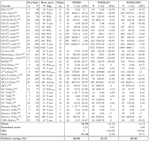
We performed the random benchmark in order to determine the average case scaling of the T-count with respect to n for each computationally efficient version of T-optimiser with results shown in Fig. 4. For both versions of TOOL, we find that the numerical results for the T count follow the expected analytical scaling of O(n2) and correspondingly the results for RE scales as O(n3). We see that TODD slightly outperforms the next best algorithm, TOOL (without feedback) and is therefore the preferred algorithm in settings where classical runtime is not an issue. Furthermore, for all compilers the distribution ofT-counts (for fixed n) concentrates around the mean value. Fig. 4 includes error bars showing the distribution but they are too small to be clearly visible, so for one data point we highlight this with an inset histogram. Therefore, TODD performs better, not just on average, but on the vast majority of random circuits so far tested. While both have a polynomial runtime, we found TOOL runs faster than TODD. Therefore, TOOL may have some advantage for larger circuits that are impractically large for TODD. However, TODD can always partition a very large circuit into several smaller circuits at the cost of being slightly less effective at reducingT count. Consequently, for very large circuits, it is unclear which compiler will work best and running both is recommended.

The random benchmark effectively uses diagonal CNOT + T circuits. This gate set is not universal and therefore is computationally limited. However, these circuits are generated by{T, CS, CCZ}, which all commute. This means such circuits lie in the computational complexity class IQP (which stands for instantaneous quantum polynomial-time) that feature in proposals for quantum supremacy experiments [26, 34, 35]. Low cost designs of IQP circuits provided by our compiler would therefore be an asset for achieving quantum supremacy.

8 10 12 14 16 18

0 100 200 300 400 500 600 700

TODD

TOOL (Without Feedback) TOOL (Feedback)

average

T

count

qubits

n

RE

50 51 52 53 54 55 56 57 58 59 0

100 200 300

T count

number of circuits

Example distribution for TODD with n₌₁₂

KEY:

60

FIG. 4. Circuits generated by the CNOT and T _{gate were randomly generated for varying number of qubits}n _{then optimized}

by our implementations of RE, TOOL and TODD. The averageT-count for eachn over many random circuits are shown on the vertical axis. TODD produces circuit decompositions with the smallestT-counts on average but scales the same as the next best algorithm, TOOL (Feedback). Both of these algorithms are better than RE by a factorn_{. The difference between the}T_{-counts for}

TODD and TOOL (Feedback) seem to converge to a constant 5.5±0.7 for largen.

B. Quantum Algorithms Benchmark

The results in Table I show that the TODD algorithm reduced or preserved theT count for every input quantum circuit upon which it was tested, as expected. Additionally, TODD yields a positive saving over the best previous algorithm for all benchmarks except Mod 54 with an average and maximum saving of 20% and 51%, respectively. This is immediately

useful due to the lower cost associated with solving these problems.

Crucially, the output circuits of our protocol often require a considerable number of ancilla qubits due to our use of Hadamard gadgets. This space-time trade-off is justifiable when the cost of introducing an additional qubit is small in comparison to that of performing an additionalT gate [39]. Furthermore, our compilers can be executed with a cap,hcap,

on the size of the ancilla register by dividing the circuit into subcircuits containing no more thanhcap Hadamard gates.

A larger number of Hadamard gates generally leads to an increased classical compilation time for TODD as well as an increasedT count for TODD-part (see appendix A), which naturally motivates future investigation into Hadamard gate optimization as a pre-processing step of TOpt-like compilers. Finally, further reductions in the space (and other) resource requirements may be possible by back-substituting the Hadamard gadget identity from Fig. 2 post-optimization.

input for the random benchmark typically have optimalT counts close to the worst-case bound ofO(n2). TODD yieldsT counts very close to optimal because it only terminates when nearly all avenues forT count reduction have been exhausted. The TOOL algorithm outputsT counts belowO(n2_{), so closely competes with TODD for random circuits. However, for}

the Clifford +T benchmark, the optimalT count is typically much less than the worst-caseO(n2) bound. It is important to recall at this stage that TOOL is optimal for the special case where the circuit implements a control-Clifford. But even for this special case, TOOL needs to know which qubit is the control qubit in order to take advantage of this special case behaviour. Consequently, a general-purpose automated compiler without prior knowledge about the input quantum circuit must have access to an additional subroutine which determines the control qubit. For general quantum circuits, the task is especially challenging because the circuit must also be optimally partitioned into a sequence of control-Cliffords. As such, we have left this task as an avenue of future work. Our implementation of TOOL uses a naive random control-qubit selection subroutine, so regardless of the low optimalT count, TOOL will often outputT counts that remain close to the worst-case ofO(n2). We suggest that this is the principle cause for the relatively poor performance seen in Table I, which has lead to negative savings not only over the best previous result and TODD, but sometimes also over the input circuit, and conclude that a better control-qubit selector would unlock more of TOOL’sT-optimizing potential.

C. The T _{Count and Other Metrics}

We acknowledge that theT count does not account for the full space-time cost of quantum computation. Recall that we justified neglecting the cost of Clifford gates due to the high ratio between the cost of theT gate and that of Clifford gates. The full space-time cost is highly sensitive to the architecture of the quantum computer, but for the surface code, this ratio is estimated to be between 50 and 1000 [12, 36–38], depending on architectural assumptions.

Note that while our protocol leads to circuits with lowT count, the final output often has anincreased CNOT count. This is largely due to step 6 of our protocol where we map the phase polynomial back to a quantum circuit using a naive approach. AlthoughT gates cost significantly more than CNOTs individually, the lower bound on number of CNOT gates required to implement high complexity reversible functions exceeds the upper bound on the number ofT gates required by an amount that grows exponentially in n[39]. So for large n, our focus should turn instead to CNOT optimization. In this paper, we focus exclusively onT count optimization, which is relevant not just to circuit optimization but also to classical simulation runtime [16, 40, 41] and distillation of magic states [24]. For this reason, we omit the CNOT count from our benchmark tables and leave the problem of optimizing CNOT count as an avenue for future work.

V. CONCLUSIONS & ACKNOWLEDGEMENTS

In this work, we have developed a framework for compiling and optimizing Clifford +T quantum circuits that reduces theT count. This scheme maps the quantum circuit problem to an algebraic problem involving order 3 symmetric tensors, for which we have presented an efficient near-optimal solver, and we have reviewed previous methods. We implemented our protocol in C++ and used it to obtainT count data for quantum circuit benchmarks. Each variant of the compiler has managed to produce quantum circuits for quantum algorithms with lowerT-counts than any previous attempts known to us. However, we find that the TODD compiler with Hadamard gadgets performs the best in practice. This lowers the cost of quantum computation and takes us closer to achieving practical universal fault-tolerant quantum computation.

TABLE I.T_{-counts of Clifford +}T_{benchmark circuits for the TODD, TOOL(F) (with feedback) and TOOL(NF) (without feedback)}

variants of the TOpt compiler are shown. Results for other variants can be seen in Table II of appendix A. Columnsnandnhshow the number of qubits for the input circuit and the number of Hadamard ancillas, respectively. TheT-count for the circuit is given: before optimization (Pre-Opt.); after optimization using the best previous algorithm (Best prev.); and post-optimization using our implementation of TODD, TOOL(F) and TOOL(NF). The best previous algorithm is given in theAlg. column where: T-par is from [20]; RMm and RMr are the majority and recursive Reed-Muller optimizers, respectively, both from [22]; and AutoH is the

heavy version of the algorithm from [21]. We show theT_{-count saving for each TOpt variant over the best previous algorithm in the} scolumns and the execution time as run on the Iceberg HPC cluster in thetcolumns. Results where the execution time is marked with† _{were obtained using an alternative implementation of TODD that is faster but less stable. The rowPositive savingshows}

the proportion of the benchmark circuits, as a percentage, for which the corresponding compiler yields a positive saving over the best previous result.

Pre-Opt. Best prev. TOpt TODD TOOL(F) TOOL(NF) Circuit n T T Alg. nh T t (s) s(%) T t (s) s(%) T t (s) s(%)

Mod 54[42] 5 28 16 T-par 6 16 0.04 0 19 0.38 −18.75 19 0.37 −18.75

8-bit adder[42] _{24 399 213 RM}

m 71 129 40914.1 39.44 279 71886.1 −30.99 284 55574.6 −33.33 CSLA-MUX3[32] 16 70 58 RMr 17 52 30.41 10.34 84 122.95 −44.83 73 84.54 −25.86 CSUM-MUX9[32] 30 196 76 RMr 12 72 587.21 5.26 83 2081.13 −9.21 104 340.19 −36.84 GF(24_)-mult[42] _{12 112 68 T-par 7 54 8.88 20.59 75 5.96}

−10.29 75 2.38 −10.29 GF(25_)-mult[42] _{15 175 101 RM}

r 9 87 66.83 13.86 109 17.6 −7.92 107 28.27 −5.94 GF(26_)-mult[42] _{18 252 144 RM}

r 11 126 521.86 12.50 165 82.52 −14.58 157 60.16 −9.03 GF(27_)-mult[42] _{21 343 208 RM}

r 13 189 2541.4 9.13 277 226.4 −33.17 209 122.17 −0.48 GF(28_)-mult[42] _{24 448 237 RM}

r 15 230 36335.7 2.95 370 379.97 −56.12 281 322.83 −18.57 GF(29_)-mult[42] _{27 567 301 RM}

r 17 295 50671.1 1.99 454 1463.02 −50.83 351 816.04 −16.61 GF(210_)-mult[42] _{30 700 410 T-par 19 350 15860.3}† _{14.63 550 7074.29}

−34.15 434 988.04 −5.85 GF(216_)-mult[42] _{48 1792 1040 T-par 31 - 1723 75204.8}

−65.67 1089 30061.1 −4.71 Grover5[42] 9 52 52 T-par 23 44 17.07 15.38 106 110.29 −103.85 83 117.39 −59.62 Hamming15(low)[42] 17 161 97 T-par 34 75 902.69 22.68 161 2787 −65.98 132 1041.22 −36.08 Hamming15(med)[42] 17 574 230 T-par 85 162 12410.8† 29.57 727 176275−216.09 277 59112.2 −20.43 HWB6[30] 7 105 71 T-par 24 51 55.66 28.17 189 140.79 −166.20 149 59.24 −109.86 Mod-Mult55[42] 9 49 35 RMm&r 10 17 0.26 51.43 35 5.45 0 19 0.92 45.71

Mod-Red21[42] 11 119 73 T-par 17 55 25.78 24.66 68 40.82 6.85 71 19.76 2.74

nth_-prime

6[30] 9 567 400 RMm&r 97 208 37348† 48 830 205869−107.50 344 135165 14 QCLA-Adder10[42] 36 238 162 T-par 28 116 5496.66 28.40 167 7544.58 −3.09 180 4560.78 −11.11 QCLA-Com7[42] 24 203 94 RMm 19 59 198.55 37.23 79 420.95 15.96 125 465.41 −32.98 QCLA-Mod7[42] 26 413 235 AutoH 58 165 46574.3 29.79 295 35249.2 −25.53 310 22355.4 −31.91 QFT4[42] 5 69 67 T-par 39 55 93.65 17.91 67 1602.91 0 59 2756.34 11.94

RC-Adder6[42] 14 77 47 RMm&r 21 37 18.72 21.28 48 1238.12 −2.13 44 81.77 6.38 NC Toff4[42] 5 21 15 T-par 2 13 <10−2 13.33 14 0.02 6.67 14 0.01 6.67

NC Toff5[42] 7 35 23 T-par 4 19 0.06 17.39 22 0.24 4.35 22 0.12 4.35

NC Toff6[42] 9 49 31 T-par 6 25 0.4 19.35 31 1146.04 0 29 0.67 6.45

NC Toff10[42] 19 119 71 T-par 16 55 44.78 22.54 65 1357.98 8.45 67 110.44 5.63

Barenco Toff4[42] 5 28 16 T-par 3 14 <10−2 12.50 16 0.02 0 16 0.03 0

Barenco Toff5[42] 7 56 28 T-par 7 24 0.45 14.29 26 0.88 7.14 27 0.56 3.57

Barenco Toff6[42] 9 84 40 T-par 11 34 1.94 15 42 12.6 −5 42 2.59 −5

Barenco Toff10[42] 19 224 100 T-par 31 84 460.33 16 120 1938.01 −20 122 1269.03 −22 VBE-Adder3[42] 10 70 24 T-par 4 20 0.15 16.67 24 1639.76 0 38 1.93 −58.33

Mean 19.76 −31.59 −14.13

Standard error 2.12 8.87 4.69

Min 0 −216.09 −109.86

Max 51.43 15.96 45.71

Positive saving (%) 96.88 18.18 30.30

[1] A. Y. Kitaev, A. Shen, and M. N. Vyalyi, Classical and quantum computation, Vol. 47 (American Mathematical Society Providence, 2002).

[2] C. M. Dawson and M. A. Nielsen, arXiv:quant-ph/0505030 (2005). [3] A. G. Fowler, Quantum Information & Computation11, 867 (2011).

[4] V. Kliuchnikov, D. Maslov, and M. Mosca, Physical review letters110, 190502 (2013). [5] P. Selinger, Physical Review A87, 042302 (2013).

[7] N. J. Ross and P. Selinger, Quant. Inf. and Comp.16, 901 (2016). [8] E. T. Campbell, B. M. Terhal, and C. Vuillot, arXiv:1612.07330 (2016). [9] S. Bravyi and A. Kitaev, Phys. Rev. A71, 022316 (2005).

[10] R. Raussendorf, J. Harrington, and K. Goyal, New Journal of Physics9, 199 (2007), arXiv:quant-ph/0703143. [11] A. G. Fowler, M. Mariantoni, J. M. Martinis, and A. N. Cleland, Phys. Rev. A86, 032324 (2012).

[12] J. O’Gorman and E. T. Campbell, Physical Review A95, 032338 (2017).

[13] A. Paetznick and K. M. Svore, Quantum Information & Computation14, 1277 (2014). [14] A. Bocharov, M. Roetteler, and K. M. Svore, Physical Review A91, 052317 (2015). [15] A. Bocharov, M. Roetteler, and K. M. Svore, Phys. Rev. Lett.114, 080502 (2015). [16] M. Howard and E. Campbell, Phys. Rev. Lett.118, 090501 (2017).

[17] E. Campbell, Physical Review A95, 042306 (2017). [18] M. B. Hastings, arXiv:1612.01011 (2016).

[19] M. Amy, D. Maslov, M. Mosca, and M. Roetteler, IEEE Transactions on Computer-Aided Design of Integrated Circuits and Systems32, 818 (2013).

[20] M. Amy, D. Maslov, and M. Mosca, IEEE Transactions on Computer-Aided Design of Integrated Circuits and Systems33, 1476 (2014).

[21] Y. Nam, N. J. Ross, Y. Su, A. M. Childs, and D. Maslov, arXiv:1710.07345 (2017). [22] M. Amy and M. Mosca, arXiv:1601.07363 (2016).

[23] G. Seroussi and A. Lempel, SIAM Journal on Computing9, 758 (1980). [24] E. T. Campbell and M. Howard, Phys. Rev. A95(2017).

[25] A. Lempel, SIAM J. Comput.4(1975).

[26] M. J. Bremner, R. Jozsa, and D. J. Shepherd, Proceedings of the Royal Society of Lon-don A: Mathematical, Physical and Engineering Sciences (2010), 10.1098/rspa.2010.0301, http://rspa.royalsocietypublishing.org/content/early/2010/08/05/rspa.2010.0301.full.pdf.

[27] A. Montanaro, Journal of Physics A: Mathematical and Theoretical50, 084002 (2017).

[28] M. Amy, D. Maslov, M. Mosca, and M. Roetteler, IEEE Transactions on Computer-Aided Design of Integrated Circuits and Systems32, 818 (2013).

[29] J. H˚astad, Journal of Algorithms11, 644 (1990).

[30] D. Maslov, “Reversible logic synthesis benchmarks page,”_{http://webhome.cs.uvic.ca/~dmaslov/}, 2011. [31] Information on the Iceberg HPC Cluster can be found here: ,https://www.sheffield.ac.uk/wrgrid/iceberg.

[32] Y. Nam, N. J. Ross, Y. Su, A. M. Childs, and D. Maslov, “GitHub for reference [21],”https://github.com/njross/optimizer. [33] M. A. Nielsen and I. L. Chuang,Quantum Computation and Quantum Information(Cambridge, 2000).

[34] A. W. Harrow and A. Montanaro, Nature549, 203 (2017).

[35] D. Shepherd and M. J. Bremner, Proceedings of the Royal Society of London A: Mathematical, Physical and Engineering Sciences465, 1413 (2009), http://rspa.royalsocietypublishing.org/content/465/2105/1413.full.pdf.

[36] R. Raussendorf, J. Harrington, and K. Goyal, New Journal of Physics9, 199 (2007). [37] A. G. Fowler, S. J. Devitt, and C. Jones, Scientific reports3, 1939 (2013).

[38] A. G. Fowler and S. J. Devitt, arXiv:1209.0510 (2012). [39] D. Maslov, arXiv:1602.02627 (2016).

[40] S. Bravyi, G. Smith, and J. A. Smolin, Phys. Rev. X6, 021043 (2016). [41] S. Bravyi and D. Gosset, Phys. Rev. Lett.116, 250501 (2016).

[42] M. Amy, “T-par GitHub,”https://github.com/meamy/t-par.

[43] To be precise, gadgets are only need for internal Hadamards. The external Hadamards that appear at the beginning and end of the circuit do not need to be replaced with Hadamard gadgets.

[44] Source code available athttps://github.com/Luke-Heyfron/TOpt.

[45] Other column pairs may be destroyed after the duplication transformation in addition to theath _andbth_{columns but only for}

Appendix A CLIFFORD + T _{BENCHMARKS FOR TODD-PART AND TODD-}h_cap

TABLE II.T-counts of Clifford +T benchmark circuits for the TODD-part and TODD-hcap variants of TOpt are shown. TODD-part uses

Hadamard-bounded partitions rather than Hadamard gadgets and ancillas and TODD-hcapsets a fixed cap,hcap, on the number of Hadamard

ancillas available to the compiler. Starting athcap= 1, we iteratively incremented the value ofhcap by 1 until obtaining the first result with

a positiveT-count saving over the best previous algorithm. The value ofhcap for which this occured is reported in thehcapcolumn, and the

number of partitions,T-count, execution time and percentage saving for this result are detailed by column group TODD-hcap. TODD-hcap

results that yield a positive saving forhcap = 0 correspond to results for TODD-part and results that requirehcap =nhHadamard ancillas

correspond to results for TODD. As we are strictly interested in intermediate values ofhcap, we omit these data and refer the reader to the

appropriate result. The number of Hadamard partitions is given by theNpcolumns. As in Table I,nis the number of qubits for the input circuit;TareT-counts: for the circuit before optimization (Pre-Opt.); due to the best previous algorithm (Best prev.); and post-optimization using variants of our compiler. The best previous algorithm is given in theAlg. column where: T-par is from [20]; RMm and RMr are the

majority and recursive Reed-Muller optimizers, respectively, both from [22]; and AutoH is the heavy version of the algorithm from [21]. We

show theT-count saving for each TOpt variant over the best previous algorithm in thescolumns and the execution time as run on the Iceberg HPC cluster in thetcolumns. Results where the execution time is marked with†_{were obtained using an alternative implementation of TODD}

that is faster but less stable. Positive savingshows the proportion of the benchmark circuits, as a percentage, for which the corresponding compiler yields a positive saving over the best previous result.

Pre-Opt. Best prev. TODD-part TODD-hcap

Circuit n T T Alg. Np T t (s) s(%) hcap Np T t (s) s(%) Mod 54[42] 5 28 16 T-par 7 18 <10−2 −12.50 1 4 16 <10−2 0 8-bit adder[42] _{24 399 213 RMm 20 283 12.63}

−32.86 13 5 212 227.81 0.47 CSLA-MUX3[32] 16 70 58 RMr 7 62 0.38 −6.90 5 3 54 3.73 6.90

CSUM-MUX9[32] 30 196 76 RMr 3 76 20.31 0 4 2 74 36.57 2.63

Cycle 173[42] 35 4739 1944 RMm 573 2625 1001.11−35.03 43 15 1939 25507.5† 0.26 GF(24_)-mult[42] _{12 112 68 T-par 3 56 0.55 17.65 0 See result for TODD-part}

GF(25_)-mult[42] _{15 175 101 RMr 3 90 6.96 10.89 0 See result for TODD-part}

GF(26_)-mult[42] _{18 252 144 RM}

r 3 132 121.16 8.33 0 See result for TODD-part

GF(27_)-mult[42] _{21 343 208 RM}

r 3 185 153.75 11.06 0 See result for TODD-part

GF(28_)-mult[42] _{24 448 237 RM}

r 3 216 517.63 8.86 0 See result for TODD-part

GF(29_)-mult[42] _{27 567 301 RM}

r 3 301 2840.56 0 8 2 295 3212.53 1.99

GF(210_)-mult[42] _{30 700 410 T-par 3 351 23969.1 14.39 0 See result for TODD-part}

GF(216_)-mult[42] _{48 1792 1040 T-par 3 922 76312.5}† _11.35

-Grover5[42] 9 52 52 T-par 18 52 0.02 0 5 4 50 0.3 3.85

Hamming15(low)[42] 17 161 97 T-par 22 113 0.53−16.49 5 6 93 2.93 4.12 Hamming15(med)[42] 17 574 230 T-par 59 322 1.57 −40 11 7 226 58.08 1.74 Hamming15(high)[42] 20 2457 1019 T-par 256 1505 16.84−47.69 13 24 1010 595.8 0.88

HWB6[30] 7 105 71 T-par 15 82 0.01−15.49 3 6 68 0.13 4.23

HWB8[30] 12 5887 3531 RMm&r 709 4187 6.53−18.58 9 110 3517 259.14 0.40 Mod-Adder1024[42] 28 1995 1011 T-par 234 1165 98.8−15.23 10 27 978 665.5 3.26 Mod-Adder1048576[42] 0 0 7298 T-par 2030 9480 89486.5† −29.90

-Mod-Mult55[42] 9 49 35 RMm&r 6 28 0.02 20 0 See result for TODD-part

Mod-Red21[42] 11 119 73 T-par 15 85 0.06−16.44 4 5 69 0.59 5.48 nth_-prime

6[30] 6 567 400 RMm&r 63 402 0.17 −0.50 2 29 384 0.98 4 nth_-prime8[30] _{12 6671 4045 RM}

m&r 774 5034 8.4 −24.45 12 105 4043 898.98 0.05 QCLA-Adder10[42] 36 238 162 T-par 6 184 223.25 −13.58 5 3 157 366.1 3.09 QCLA-Com7[42] 24 203 94 RMm 7 135 11.62−43.62 16 2 81 170.77 13.83 QCLA-Mod7[42] 26 413 235 AutoH 15 305 34.76−29.79 23 3 221 289.77† 5.96

QFT4[42] 5 69 67 T-par 38 67 <10−2 0 2 13 63 0.02 5.97

RC-Adder6[42] 14 77 47 RMm&r 13 59 0.11−25.53 6 3 45 0.97 4.26 NC Toff3[42] 5 21 15 T-par 3 15 <10−2 0 2 =nh See result for TODD

NC Toff4[42] 7 35 23 T-par 5 23 <10−2 0 4 =nh See result for TODD

NC Toff5[42] 9 49 31 T-par 7 31 0.01 0 5 2 29 0.2 6.45

NC Toff10[42] 19 119 71 T-par 17 71 0.74 0 10 3 69 12.48 2.82

Barenco Toff3[42] 5 28 16 T-par 4 22 <10−2 −37.50 2 2 14 <10−2 12.50 Barenco Toff4[42] 7 56 28 T-par 8 38 0.01−35.71 4 2 26 0.06 7.14

Barenco Toff5[42] 9 84 40 T-par 12 54 0.03 −35 6 2 38 0.35 5

Barenco Toff10[42] 19 224 100 T-par 32 134 2.27 −34 16 2 98 54.75 2 VBE-Adder3[42] 10 70 24 T-par 5 36 0.04 −50 4 =nh See result for TODD

Mean −13.19 9 4.05

Standard error 3.15 1.65 0.64

Min −50 1 0

Max 20 43 13.83

In order to investigate the relative effectiveness of the Hadamard gadget and Hadamard-bounded partition methods for dealing with Hadamard gates, we repeated the benchmarks from Table I but for the latter method. The results are shown in the TODD-part column group of Table II. For the Hadamard partition method, we found that the compiler runtime is significantly decreased, making the optimization of larger quantum circuits feasible. However, the performance is worse in terms of rawT count reductions, often leading to higher T counts than the best previous result. It is important to note that for a given input circuit, theT count is highly sensitive on the choice of Hadamard partitioning, of which, in general, there are many. Our implementation does not optimize over Hadamard partitioning choices, so there is potential for developing a more powerful version of TODD-part that makes use of an advanced Hadamard partitioning algorithm, which may lead to greaterT count reductions.

The TODD compiler completely gadgetizes each Hadamard gate, whereas the TODD-part compiler completely partitions the circuit into Hadamard-bounded partitions. It is possible to interpolate between these two approaches using a parameter hcapthat enforces a cap on the number of available Hadamard ancillas. Upon reaching this cap, the compiler synthesises the

circuit encountered so far, freeing up the Hadamard ancillas for the subsequent Hadamard partition. We have implemented this feature, and in order to quantify the overhead required to see aT count reduction, we ran each benchmark repeatedly, incrementing the value of hcap until we saw a reduction over the best previous result. The results for this experiment

are presented in Table II. We found that the relationship betweenhcapand T count savings is favourable: relatively few

Hadamard gadgets are required to see a reduction over the best previous result. Over all the benchmark circuits, where the number of qubits and the T count ranges up to n = 36 and T = 6671, respectively, we found that on average 9 Hadamard ancillas are required to see positive saving and at most 23 ancillas are needed for all but one exceptional result (Cycle 173), which requires 43. This suggests that, while TODD combined with full Hadamard gadgetization is clearly

the forerunner amongst our compilers for reducing the T count, a modest improvement in the Hadamard partitioning scheme, or adding a pre-processing step that looks for Hadamard gate reductions may lead to a better version of TODD that requires no non-unitary gadgets, has feasible compiler runtimes for large circuits, and yields positiveT count savings.

Appendix B LEMPEL’S FACTORING ALGORITHM

We describe Lempel’s factoring algorithm (originally from reference [25]) using conventions consistent with our descrip-tion of the TODD algorithm to more easily see how TODD generalizes Lempel’s algorithm for order 3 tensors. Lempel’s factoring algorithm takes as input a symmetric tensor of order 2 (a matrix), which we denoteS ∈Z(2n,n) and outputs a

matrixA∈Z(2n,m)where the elements of AandS are related as follows:

Sα,β =

m

X

k=1

Aα,kAβ,k (mod 2). (32)

Lempel proved that the minimal value ofmis equal to

µ(S) =ρ(S) +δ(S), (33)

whereρ(S) is the rank of matrixS and

δ(S) =

(

1 ifSα,α= 0 ∀α∈[1, n]

0 otherwise . (34)

Lempel’s algorithm solves the problem of finding an A matrix that obeys equation (32) for a givenS matrix such that m=µ(S). Such anAmatrix is referred to as a minimal factor ofS.

In the following, we denote the number of columns ofAasc(A) and thejth _{column ofAasc}

j(A). Lempel’s algorithm

is the following:

1. Generate an initial (necessarily suboptimal)Amatrix for S.

2. Check ifc(A) =µ(S). If true, exit and outputA. Otherwise, perform steps 3 to 7. 3. Find ay∈Zm2 such thatAy=0and 0<|y|< c(A).

4. If|y|= 1 (mod 2) then updatey→(yT,1)T _{andA= (A 0).}

5. Find a pair of indicesa, b∈[1, m], a=6 b such thatya⊕yb= 1.

6. Apply transformationA→A⊕zyT, wherez=ca(A)⊕cb(A).

7. Remove theath _andbth _{columns fromA, then go to step 2.}

Note that the key difference between the Lempel and TODD algorithm is that TODD additionally requires condition

Appendix C TOOL ALGORITHM

Here we give a detailed description of TOOL, with the main idea illustrated by Fig. 3. TOOL is best explained in terms of weighted polynomials (recall equation (6)). The algorithm is iterative, where each round consists of the five steps detailed below. Before the first round, we initialize an ‘empty’ output gate synthesis matrix,Aout∈Z(2n,0).

1. Choose an integer c ∈[1, n] such that there is at least one term in f with xc as a factor. If no such c exists, the

algorithm terminates and outputsAout.

2. Find ˜fc, thetarget polynomial off with respect toxc (see equation 35 below).

3. Determine the order 2 signature tensor, ˜S, of ˜fc.

4. Find ˜A, a minimal factor of ˜S, using Lempel’s factoring algorithm.

5. Recover an order 3 gate synthesis matrix,A, for ˜A, and append it toAout. Replacef with f− |ATx|.

Each round of TOOL gives a newf that depends on fewerxvariables. Whenf depends on onlynRM or fewer variables,

we switch to the optimal brute force optimizer, RM.

We will now explain each step of the above description in detail, unpacking the contained definitions. In step 1, we select an indexc, which corresponds to the control qubit of the control-U_{2 ˜f}

c operator shown in Fig. 3. The order that we

choosecfor each round can affect the output and therefore is a parameter of TOOL. For all results, we randomly selected cwith uniform probability from the set of all indices{c}for whichxc is a factor of at least one term inf.

Next, we observe that anyf can be decomposed intof =fc+fc′, where we definefcas a weighted polynomial containing

all terms off withxc as a factor. The former part,fc, can be further decomposed as follows,

fc= 2xcf˜c+lcxc (35)

where ˜fc is quadratic and so can be optimally synthesized efficiently. In step 2, we extract ˜fc, which is implicitly fixed by

the above equations. We refer to ˜fc as atarget polynomial because it corresponds to the target of a control-U2f operator,

wheref = ˜fc and|xciis the control qubit.

As an aside, we remark that the target polynomial is related to Shannon cofactors that appear in Boole’s expansion theorem. Specifically, we have

˜

fc =

fc+−fc−−lc

2 , (36)

wheref+

c andfc− are the positive and negative Shannon cofactors, respectively, off with respect toxc, andlcis the linear

coefficient off associated with xc.

In step 3, we map ˜fc to a signature tensor of order 2 (a matrix) for use with Lempel’s factoring algorithm. Let ˜lα,q˜α,β

be the linear and quadratic coefficients of ˜fc, respectively. For eachα, β6=c, the elements of ˜S are obtained as follows.

˜

Sα,β=

(

˜

lα (mod 2) if α=β

˜

qα,β (mod 2) if α6=β

. (37)

Finding a minimal factor of ˜Sα,β is the problem 2-STR. Therefore, we can use Lempel’s algorithm (see appendix B) to

find a matrix ˜A∈Z(2n,m˜), which is a minimal factor of ˜S such that

˜

fc=|A˜Tx|=

˜ m

X

j=1

" _n M

i=1

˜

Ai,jxi

#

(mod 8). (38)

By substituting equation (38) into equation (35) we obtain

fc= 2xc|A˜Tx|+lcxc, (39)

=

˜ m

X

j=1

2xc

" _n M

i=1

˜

Ai,jxi

#

where we have taken the factor 2xc within the Hamming weight summation. Next, we use the modular identity 2ab =

a+b−a⊕bwitha=xc andbas the contents of the square brackets. This gives

fc =

˜ m

X

j=1

xc+

" _n M

i=1

˜

Ai,jxi

# −xc⊕

" _n M

i=1

˜

Ai,jxi

#!

+lcxc (mod 8), (41)

=xc( ˜m+lc) + ˜ m

X

j=1

" _n M

i=1

˜

Ai,jxi

# −

˜ m

X

j=1

xc⊕

" _n M

i=1

˜

Ai,jxi

#

(mod 8), (42)

=xc( ˜m+lc) +|A˜Tx| − |( ˜A⊕Bc)Tx| (mod 8), (43)

whereBc ∈Z (n,m)

2 is a matrix with elements

[Bc]_i,j=

(

1 ifi=c

0 otherwise. (44)

This is now in the form of a phase polynomial (e.g. see equation (8)) with no more than 1 + 2 ˜mterms, where ˜mwas the optimal size of the factorisation found using Lempel’s algorithm.

There are two versions of TOOL: with and without feedback. The difference between these versions determines whether all of equation (43) is put intoAoutor whether parts are ‘fed back’ intof for subsequent rounds. This leads to two distinct

definitions of theAmatrix referred to in step 5 of TOOL:

|ATx|=

(

( ˜m+lc)xc− |( ˜A⊕Bc)Tx| feedback

( ˜m+lc)xc− |( ˜A⊕Bc)Tx|+|A˜Tx| without feedback

. (45)

Notice that both ( ˜m+lc)xc and |( ˜A⊕Bc)Tx| depend on xc, so must be sent to output. Furthermore, they comprise

all the terms that depend on xc, which is why sending|A˜Tx| to output is optional, and why the number of dependent

variables is reduced by at least 1 each round. For thefeedback version,|A˜T_{x|is kept withinf during step 5, whereas it is}

sent to outputAout in the without feedback version.

Appendix D CALCULATING CLIFFORD CORRECTION

We will now describe how to determine the Clifford correction required to restore the output of T-Optimiser to the input unitary. Let the input ofT-Optimiser be a weighted polynomialf that implements unitary Uf ∈ D3, and let the

output be a weighted polynomialg. Anyf can be split into the sum

f =f1+f2, (46)

where the coefficients off1are inZ2and those off2are even. From the definition ofT-Optimiser, we know the coefficients

off andghave the same parity i.e.

g=g1+g2=f1+g2, (47)

whereg1, g2are similarly defined for g. Using equations (46) and (47) we find,

g=f + (g2−f2). (48)

Equation (48) implies thatUClifford=U(g2−f2)∈ D2. Therefore, the Clifford correction isU_Clifford† =U₍†_g2−f2)=U(f2−g2).

Appendix E TODD PSEUDOCODE

Algorithm 1Third Order Duplicate-then-Destroy (TODD) Algorithm

Input: Gate synthesis matrixA∈Z(2n,m). Output: Gate synthesis matrixA′

∈Z(2n,m′) such thatm ′

≤m_andS(A′₎

=S(A)_.

• Let colj(A) be a function that returns thejthcolumn ofA.

• Let cols(A) be a function that returns the number of columns ofA.

• Let nullspace(A) be a function that returns a matrix whose columns generate the right null space of A.

• Let proper(A) be a function that returns matrixAwith every pair of identical columns and every all-zero column removed.

procedureTODD

InitializeA′ _←A start:

for all1≤a < b≤cols(A′)do

z←cola(A′) + colb(A′)

˜

A←





A′

χ(A′_,z)





N←nullspace( ˜A)

for all1≤k≤cols(N)do

y←colk(N)

if ya⊕yb= 1then

if |y|= 1 (mod 2)then

A′_←

A′ 0

y←



 y

1





A′←A′+zyT

A′←proper(A′₎ goto start

Appendix F COMPUTATIONAL EFFICIENCY OF TODD

In this appendix, we calculate an upper-bound on the worst-case computational efficiency of the TODD algorithm as described in appendix E, in terms of the number of arithmetic operations onGF(2) required.

LetAbe a gate synthesis matrix withnrows andmcolumns that is used as input for the TODD algorithm. The loop, L1, over each column pair (a, b) requires at most m₂=O(m2) iterations to complete. InsideL1, there are four lines of

pseudocode: a column addition, requiring no more thannoperations; a matrix concatenation and calculation of χ(A,z), requiringE1 operations; a nullspace calculation, requiring O(n3) +O(m2n) operations using Gaussian elimination; and

finally a nested loopL2, requiringE2 operations.

From equation (27), we see that each row ofχ(A,z) can be calculated withO(m) operations. There are a maximum of

n 3

rows inχ(A,z) so the total number of operations required to calculateχ isO(n3m). Combining this with the matrix concatenation, we find thatE1=O(n3m) +nm=O(n3m).

The loopL2 executes in at most

cols₍nullspace_{( ˜A)) :=}colrank₍nullspace_{( ˜A)) =m−}rank_{( ˜A)≤m−}rank_{(A)≤m−n (49)}

iterations. The identity between the column rank and the number of columns follows from the assertion that the nullspace function outputs a matrix whose columns are a linearly independent basis for the nullspace ofA.

The loopL2is composed of a conditional that requires 1 addition (by merging the first line ofL2 and the conditional).

The content of the conditional is only evaluated once, so can be considered as part ofL1 for this calculation. Therefore,

the number of operations performed inL2 isE2=m−n.

The nested conditional requires at mostm+n+ 1 operations, where the terms are due to the Hamming weight of|y|, concatenating an all-zero column to A′ _{and concatenating a one to y, respectively. The line A}′ _{← A}′ _+zyT _requires

at most n(m+ 1) operations and the proper function can be computed using at most moperations by keeping track of all-zero columns with a Boolean array, for a small physical overhead ofm.