This is a repository copy of
A Conformal Thin Boundary Model for FDTD
.
White Rose Research Online URL for this paper:
http://eprints.whiterose.ac.uk/131594/
Version: Accepted Version
Proceedings Paper:
Bourke, Samuel, Dawson, John orcid.org/0000-0003-4537-9977, Robinson, Martin
orcid.org/0000-0003-1767-5541 et al. (1 more author) (2018) A Conformal Thin Boundary
Model for FDTD. In: 2018 IEEE MTT-S International Conference on Numerical
Electromagnetic and Multiphysics Modeling and Optimization for RF, Microwave, and
Terahertz Applications (NEMO) (NEMO2018). .
https://doi.org/10.1109/NEMO.2018.8503410
[email protected] https://eprints.whiterose.ac.uk/
Reuse
Items deposited in White Rose Research Online are protected by copyright, with all rights reserved unless indicated otherwise. They may be downloaded and/or printed for private study, or other acts as permitted by national copyright laws. The publisher or other rights holders may allow further reproduction and re-use of the full text version. This is indicated by the licence information on the White Rose Research Online record for the item.
Takedown
If you consider content in White Rose Research Online to be in breach of UK law, please notify us by
A Conformal Thin Boundary Model for FDTD
Samuel Bourke, John Dawson, Martin Robinson, Stuart Porter
Department of Electronic Engineering University of York
York, UK
samuel.bourke, john.dawson, martin.robinson, [email protected]
Abstract—Thin layer models are widely used in the
finite-difference time-domain (FDTD) technique to efficiently model boundaries in multi-scale simulations as they significantly reduce simulation run-times and memory requirements. These models often utilise surface impedance boundary conditions (SIBCs) to represent the material of the boundary. Conformal meshes are a popular method of representing curved and non-aligned surfaces in FDTD. These meshes deform cells in the FDTD grid around the boundary between bulk materials so as to more accurately repre-sent the shape of the material. Here we prerepre-sent an algorithm that combines the efficiency of a thin layer model with the accuracy of a conformal mesh. The algorithm is applied to three resonant cavity models and the accuracy verified using comparisons to non-conformal meshes and analytic solutions. Improvements are shown in the accuracy of the resonant frequencies and magnitude of the shielding effectiveness (SE) of the cavities. It is also shown to reduce the prevalence of extraneous features in the frequency response of the SE that are apparent when using a stair-cased mesh.
Index Terms—Finite-Difference Time-Domain, Conformal
Techniques, Surface-Impedance Boundary Condition, Thin Layer
I. INTRODUCTION
FDTD is a popular numerical method for solving Maxwell’s equations [1]. The strength of the method lies in its efficiency and simplicity. Being a time domain algorithm it is possible to solve problems over a large range of frequencies in a single simulation.
Surface Impedance Boundary Conditions (SIBCs) are useful tools that can be used to model very thin materials [2], [3]. They allows a material that is much thinner than the size of the mesh to be simulated without having to simulate the field inside the material. Instead, they use a behavioural model that controls how the material interacts with the mesh. Doing this can reduce simulation run-times significantly [4].
However it is commonly known that FDTD can suffer from inaccuracies due to its reliance on a cuboid grid. Surfaces that are curved, or do not align with the grid, cannot be accurately represented and are commonly approximated using a stair-cased mesh. This can introduce a number of errors into the results of the algorithm [5]. A popular solution to this problem is the introduction of conformal algorithms. These algorithms deform individual cells in the cuboid grid to
This work was undertaken with funding from COST Action IC1407 (ACCREDIT) and EPSRC Studentship 1642594.
better conform to non-aligned and non-orthogonal geometries. Early conformal algorithms could be used to represent perfect electrical conductors [6], [7] and later methods allowed for conformal meshes of penetrable materials [8]. Current confor-mal algorithms rely on meshing bulk materials, where the field inside the material is simulated on the FDTD grid. This means that having a bulk conformal material boundary also means having a larger simulation to account for the cells inside the material.
In this paper we propose a conformal algorithm that utilises a SIBC for representing curved and non-aligned planar sur-faces in FDTD. This combines the efficiency of using a thin boundary model and the accuracy of using a conformal mesh. The algorithm is proposed in Section II and validated using different cavity models in Sections III, IV and V. Conclusions about the approach are presented in Section VI
II. PROPOSEDCONFORMALALGORITHM
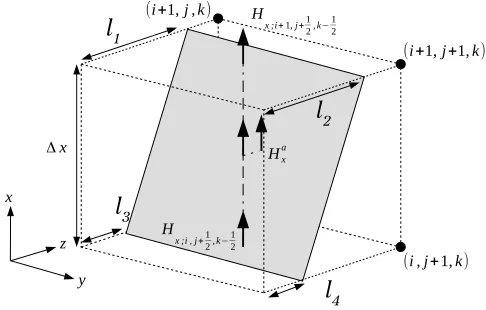
[image:2.612.317.560.498.653.2]Here the adaptation of an existing SIBC [3] to a conformal mesh is described. Consider the cell in Fig. 1, the shaded boundary has been moved from the xy-plane face at i towards the centre to conform with a surface passing through the cell, by directly modifying a stair-cased surface mesh.. Where l1,l2,l3andl4are the distance that each corner of the boundary has moved.
Fig. 1. Conformal algorithm applied to a single cell. The shaded surface is not parallel to any cell face.
The original SIBC uses spatial interpolation to approximate the magnetic field at the centre of the SIBC parallel to the
978-1-5386-5204-6/18/$31.00 ©2018 IEEE
© 2018 IEEE. Personal use of this material is permitted. Permission from IEEE must be obtained for all other uses, in any current or future media, including
face, on the mesh cell surface. This is achieved by averaging the magnetic fields on the surface of the cell:
Hxa= Hn−12
x;i,j+1
2,k−12 +H
n−12
x;i+1,j+1 2,k−12
2 (1)
To apply a conformal SIBC the magnetic fields must be weighted according to their distance to the boundary, so (1) becomes:
Ha x =
1
2(δ1+δ2)H n−12
x;i,j+1 2,k−12
+1
2(δ3+δ4)H n−12
x;i+1,j+1 2,k−12
2
(2)
Whereδ1,δ2,δ3 andδ4 are the fractional edge lengths:
δn= ln
∆z (3)
Similar update equations can be derived for determining the y-polarised magnetic field.
The usual FDTD equations are used to update the surround-ing magnetic field components ussurround-ing the electric fields on the SIBC surface modified by the average fractional edge length:
Hn+12
x;i,j+1 2,k−12 =
Hn−12
x;i,j+1 2,k−12
+Chxe i,j+1
2,k−12
1 ∆zk
n
1
2(δ2+δ3)E a;n y;i,j+1
2,k− En
y:i,j+1 2,k−1
o
+ 1 ∆yj
n
En
z;i,j,k−12 −E
n
z:i,j+1,k−12 o
(4)
Where Chxe
i,j+1
2,k−12 is the standard magnetic field update
coefficient [9]. Again, similar update equations can be derived for the y-polarised magnetic fields. Any yz-plane and zx-plane faces on the staircase mesh in the cell are dealt with in the same way and the sum of the coincident boundaries add to give the correct overall behaviour.
III. 1D RESONATORTESTCASE
The first validation test for the proposed algorithm is a simple 1D resonator. This test consists of two thin planar boundaries separated by 3.95m of free space. The bound-aries are isotropic and symmetrical with constant transmission and reflection coefficients of 0.004 and -0.99 respectively. A Gaussian pulse is used to illuminate the resonator at normal incidence from the left as shown in Fig. 2.
The electric field at a given point in the cavity can be determined analytically as:
E(x) = EIτ(e−
γx+
ρe−γ(2d−x)) 1−ρ2e−2γd
(5)
whereEI is the magnitude of the incident electric field,x
is the distance from the left side of the cavity, dis the length
[image:3.612.306.565.50.130.2]of the cavity, γ is the propagation constant andτ andρ are
Fig. 2. 1D Resonator Diagram.EIis the incident electric field andsis the
direction of propogation.
the transmissions and reflection coefficients of the boundaries respectively.
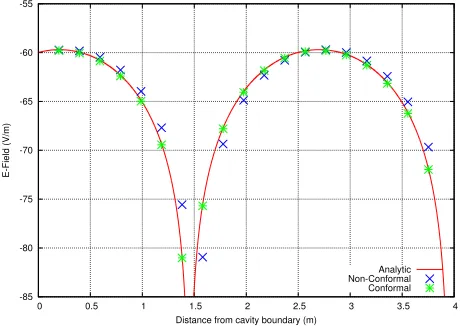
The initial simulation for this problem uses a cavity length of 3.95m and a mesh size of 0.2m. This means that, when using a non-conformal mesh, the cavity length must be a mul-tiple of 0.2m and therefore the cavity modelled is effectively 4m long. When using the conformal mesh one cell can be deformed allowing a 3.95m long model while using a 0.2m global mesh size. The electric field along the cavity at 37MHz is shown in Fig 3.
-85 -80 -75 -70 -65 -60 -55
0 0.5 1 1.5 2 2.5 3 3.5 4
E-Field (V/m)
Distance from cavity boundary (m)
[image:3.612.319.549.314.477.2]Analytic Non-Conformal Conformal
Fig. 3. E-Field along 1D Cavity at 37MHz. Comparison of analytic solution with conformal and non-conformal meshes.
It can be seen that for the non-conformal case the field is shifted slightly in space, however when using the conformal mesh this has been corrected and the field values lie on the analytic curve.
0 0.5 1 1.5 2 2.5 3 3.5 4 4.5 5
3.8 3.82 3.84 3.86 3.88 3.9 3.92 3.94 3.96 3.98 4
Error in SE (%)
Error in Resonant Frequency (%) Non-Conformal
[image:4.612.57.283.53.216.2]Conformal
Fig. 4. Error in resonant frequency for 1D cavities of different widths. The number of cells across the cavity and the mesh size remain constant.
IV. CUBICSHELLTESTCASE
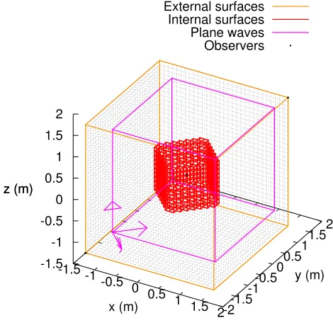
To test the conformal algorithm on a three dimensional problem, a cubic cavity is investigated. It is possible to mesh a cubic shell so that it aligns perfectly with the grid, obviating the need for a conformal mesh. However, if the cube is not aligned with the mesh it may become necessary to use a conformal, or stair-cased, mesh to represent the faces of the cube as shown in Fig. 5.
-1.5 -1 -0.5 0
0.5 1
1.5 2-2-1.5
-1-0.5
0 0.5
1 1.5
2
-1.5 -1 -0.5 0 0.5 1 1.5 2
z (m)
External surfaces Internal surfaces Plane waves Observers
x (m)
[image:4.612.320.547.136.296.2]y (m) z (m)
Fig. 5. Mesh of cubic shell.
In this case the cube has been rotated around a single axis causing four of the faces to become misaligned and require a stair-cased mesh. The cube is illuminated using a vertical, linearly polarised plane wave, at normal incidence to the face of the cube. The electric field at the centre of the cube is monitored. From this the shielding effectiveness (SE) at the
centre of the cube is determined and shown in Fig. 6. Here the SE is the ratio of the external and internal electric field strength. As there is no analytic solution for a cubic shell, a simulation of the cube that is aligned to the FDTD grid is used for comparison. For the aligned case no stair-casing is needed and the conformal mesh reduces to the standard algorithm.
0 10 20 30 40 50 60 70
0 100 200 300 400 500
SE (dB)
Frequency (MHz)
Θ = 0
Non-Conformal Θ = 45
Conformal Θ = 45
Fig. 6. Shielding effectiveness at the centre of a cubic shell rotated 45°with respect the the FDTD grid. Comparisons are made with an aligned case.
[image:4.612.58.293.387.620.2]There is a significant improvement in the accuracy mag-nitude of the SE using the conformal mesh when compared to the stair-cased mesh, reducing the error from 7dB to approximately 1.5dB. A close up of the first resonance in Fig. 7 shows an error in the resonant frequency for the stair-cased mesh of around 1%, when using the conformal mesh this is reduced to approximately 0.1%. Although the resonant frequency is more accurate with the conformal mesh the amplitude error suggests there is still some inaccuracy in the transmission and reflection coefficients achieved. This will be further investigated in the future.
6 7 8 9 10 11 12 13 14 15
210 211 212 213 214 215
SE (dB)
Frequency (MHz)
Θ = 0
Non-Conformal Θ = 45
Conformal Θ = 45
Fig. 7. Shielding effectiveness at the first resonant frequency of a cubic shell.
V. CYLINDRICALSHELLTESTCASE
[image:4.612.320.547.481.643.2]infinite cylindrical cavity is meshed with a radius of 1m using the same boundary conditions as the previous test cases. Again the cavity is illuminated using a linearly polarised plane wave, with the incident electric field being polarised along the x-axis. Perfect Magnetic Conductor (PMC) boundaries are utilised at each end of the cylinder to simulate an infinitely long structure. The mesh size for this problem is 0.1m.
-1.5 -1
-0.5 0
0.5 1
1.5-1.5 -1
-0.5 0
0.5 1
1.5
-0.1 -0.05 0 0.05 0.1 z (m)
External surfaces Internal surfaces Plane waves Observers
x (m)
y (m) z (m)
Fig. 8. Stair-cased mesh of an infinite cylinder for FDTD. Only one layer of cells in required in the Z-direction, PMC boundaries emulate an infinite length.
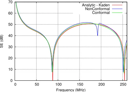
Again the E-field and subsequently SE is measured at the centre of the cavity, in this case there is an analytic solution [10] that can be used for comparison. The results are shown in Fig. 9
0 10 20 30 40 50 60 70
0 50 100 150 200 250
SE (dB)
Frequency (MHz)
[image:5.612.63.270.146.284.2]Analytic - Kaden NonConformal Conformal
Fig. 9. Shielding effectiveness at the centre of a cylindical cavity.
For the non-conformal mesh there is a clear resonance around 180MHz, this is not a spurious peak, rather it corre-sponds to a resonant mode that has a node at the centre of the cavity. For points within the cavity that are not exactly at the centre this resonance would be visible in the SE, the imprecise stair-cased approximation makes the centre of the mesh a slightly ambiguous position causing this resonance to become apparent at the centre as well. Using the conformal mesh has reduced this resonance significantly, making it almost non-existent at the centre of the cylinder. However, it should be noted that there is still a slight variation in the SE around this
frequency as the conformal mesh is still an approximation, albeit a more accurate one than the stair-cased mesh.
The error in the first resonant frequency is around 1.9% when using the stair-cased mesh, using the conformal mesh gives an error of approximately 0.4%. The error in magnitude at 50MHz is approximately 0.9dB using the stair-cased mesh, this error is improved to approximately 0.3dB using the conformal mesh.
It is worth mentioning that for the stair-cased mesh the extra resonance could be reduced, and the overall accuracy in frequency increased, using a higher resolution mesh. However, to achieve a similar result to the conformal mesh the runtime would be increased by a factor of 125. There would also be no improvement in the magnitude of the SE as errors in the boundary transmission and refection due to stair-casing are independent of mesh size [5].
VI. CONCLUSION
A new algorithm for FDTD has been presented combining a surface impedance boundary with a conformal mesh. Multiple test cases have been introduced that demonstrate the new algorithm leads to improvements in accuracy, both in the frequency of resonant modes and the magnitude of shielding effectiveness of the cavities. We have demonstrated that the conformal thin layer algorithm can also be used to reduce and potentially eliminate the presence of extraneous resonances that occur using stair-cased meshing. The method is also easy to mesh as an existing staircase mesh is modified using information on the face position in each cell.
REFERENCES
[1] K. Yee, “Numerical solution of initial boundary value problems in-volving Maxwell’s equations in isotropic media,” IEEE Transactions on Antennas and Propagation, vol. 14, pp. 302–307, May 1966. [2] V. Nayyeri, M. Soleimani, and O. Ramahi, “A method to model
thin conductive layers in the finite-difference time-domain method,” Electromagnetic Compatibility, IEEE Transactions on, vol. 56, pp. 385– 392, April 2014.
[3] I. D. Flintoft, S. A. Bourke, J. F. Dawson, J. Alvarez, M. R. Cabello, M. P. Robinson, and S. G. Garcia, “Face-centered anisotropic surface impedance boundary conditions in FDTD,”IEEE Transactions on Mi-crowave Theory and Techniques, vol. PP, no. 99, pp. 1–8, 2017. [4] J. Maloney and G. Smith, “The use of surface impedance concepts in
the finite-difference time-domain method,”Antennas and Propagation, IEEE Transactions on, vol. 40, pp. 38–48, Jan 1992.
[5] S. A. Bourke, J. F. Dawson, I. D. Flintoft, and M. P. Robinson, “Errors in the shielding effectiveness of cavities due to stair-cased meshing in FDTD: Application of empirical correction factors,” in 2017 International Symposium on Electromagnetic Compatibility - EMC EUROPE, pp. 1–6, Sept 2017.
[6] S. Dey and R. Mittra, “A modified locally conformal finite-difference time-domain algorithm for modeling three-dimensional perfectly con-ducting objects,” Microwave and Optical Technology Letters, vol. 17, no. 6, pp. 349–352, 1998.
[7] S. Benkler, N. Chavannes, and N. Kuster, “A new 3-D conformal PECFDTD scheme with user-defined geometric precision and derived stability criterion,” IEEE Transactions on Antennas and Propagation, vol. 54, pp. 1843–1849, June 2006.
[8] W. Yu and R. Mittra, “A conformal finite difference time domain technique for modeling curved dielectric surfaces,” IEEE Microwave and Wireless Components Letters, vol. 11, pp. 25–27, Jan 2001. [9] S. D. Gedney,Introduction to the finite-difference time-domain (FDTD)
method for electromagnetics. Morgan & Claypool, 2011.
[image:5.612.58.282.395.558.2]