Stability indicator of orbital motion around asteroids with automatic domain splitting

1

Stability indicator of orbital motion around asteroids with automatic

domain splitting

Feng J.1_{, Santeramo D.}2_{,Di Lizia P.}2_{, Armellin R.}3_{, Hou X.}4

1 _{University of Strathclyde, UK, [email protected]}

2 _{Politecnico di Milano, Italy} 3 _{University of Surrey, UK}

4 _{Nanjing University, China}

Abstract

Asteroids usually have irregular gravity field due to their non-spherical shapes. Moreover, their gravity fields are estimated with large uncertainty as a result of the limited ground observations. Resultantly, the orbital motion in their vicinity can be highly unstable and cannot be predicted accurately before reaching the asteroid. Therefore, the identification of stable orbital motion around asteroids is essential for robust mission design. In this study, the automatic domain splitting method (ADS) is introduced as a new tool of identifying the stable and unstable region in the phase space with gravity uncertainty. The ADS is actually based on the differential algebra (DA) method that approximates the dynamics with arbitrary order Taylor expansion and can replace thousands of pointwise integrations of Monte Carlo runs with the fast evaluation of the Taylor polynomials. The asteroid Steins is taken as an example. However, as the C20 and C22 harmonic terms are usually dominant over the non-spherical gravity, only their uncertainties are considered in the investigations. Given the required accuracy, the expansion order and the maximum splitting times are firstly determined, to balance efficiency. It is found that the orbital motion is more sensitive to the variation of the C22 term, compared with that of the C20 term. Then, the first split time of the orbits with different geometry is recorded on the semi-major axis and inclination plane, i.e. the a-i plane. Along the propagation, the bounds of the state flow are evaluated. Resultantly, given the allowed first split time and bounds that are determined according to the real mission requirement, practical stable regions can be identified.

2

1.

Introduction

Asteroids usually have irregular gravity field due to their non-spherical shapes. Moreover, their gravity fields are estimated with large uncertainty as a result of the limited ground observations. Resultantly, the orbital motion in their vicinity can be highly unstable and cannot be predicted accurately before the spacecraft arriving there. Therefore, the identification of stable orbital motion around asteroids is essential for robust mission design.

Nonlinear dynamics has been extensively addressed [1]. Nevertheless, the analysis of the effect of uncertain gravity field on orbital propagation is very limited, which is the focus of this study. The conventional methods either use the Lyapunov stability of the linearized dynamics or apply the pure numerical Monte Carlo simulations [2]. However, the limitations are that the dynamics is highly non-linear for the first method and the computational effort is heavy for the second one. Due to the increasing requirement on the on-board autonomy, (e.g., to save control effort of the nominal orbit as a result of the inaccurate estimation of the central body’s gravity) more efficient methods should be introduced and investigated.

Therefore, in this study, the automatic domain splitting method (ADS) [3] is introduced as a new tool of identifying the stable and unstable region in the phase space with gravity uncertainty. The ADS is actually based on the differential algebra (DA) method that approximates the dynamics with arbitrary order Taylor expansion and can replace thousands of pointwise integrations of Monte Carlo runs with the fast evaluation of the Taylor polynomials [4]. The computational time is reduced considerably by replacing thousands of integrations with algebra operations, while the accuracy can be kept arbitrarily high by adjusting the expansion order of the Taylor expansion. DA has been used in asteroid encounter analysis [5], orbit conjunction analysis [6], and the impact of asteroid’s gravity uncertainty on orbital propagation [7] etc.

3

perturbation for low-altitude motion around massive small bodies such as Stein [1, 8]. Moreover, the solar gravitation is generally estimated two orders of magnitude smaller than that of the SRP [8]. Therefore, both of them are not included in this preliminary work and only the non-spherical gravity is accounted for. Therefore, in the current study, the effect of the uncertain gravity field on the state propagation will be the focus. In addition, the spherical harmonics model is applied, as it is a generalized representation of the gravity field of a small body. Since the C20 and C22 are the dominant terms of the non-spherical gravity, their uncertainties are believed to contribute most to the gravity uncertainty, and are the only uncertainties considered in this study. Nevertheless, it will not be difficult to generalize this work to uncertainties on higher-order harmonic terms.

This work contributes to identify the stability of orbit motion in phase space, and to identify the practical stable region if there is no split occur during the propagation process, in a systematical and efficient way. The paper is organized as follows. Section 2 introduces the basic idea and knowledge of the ADS algorithm. Section 3 describes the dynamic model of orbital motion around an asteroid and applies the DA algorithm to expand the dynamical flow to high orders w.r.t. the gravity uncertainty. Based on large amounts of numerical simulations, the preferable orbital geometry for robust motion is analyzed in Section 4. Section 5 concludes this study and gives prospects for future research.

Figure 1 Illustration of the propagation process with ADS [3]

2.

Methodology

4

at which the flow expansion over a given initial set is not capable of describing the dynamics with the required accuracy anymore, by applying an automatic algorithm. Once this situation is detected, the domain of the original polynomial expansion is divided along one of the expansion variables into two domains of the same size. Then, the dynamics is re-expanded around the new center points of the two domains, respectively, resulting in two separate polynomial expansions. Since the new expansions do not change the order, each of the new polynomials is identical to the original ones on its respective domain. This process is illustrated in Fig.1.

Specifically, all splits are performed in the direction of the variable that contributes most to the truncation error of the polynomial, thus to maximize the reduction of the expansion error maximally. During the splitting process, the split direction strongly depends on theparametrization of the initial condition and can occur automatically along all variables that contribute to the truncation error. However, the initial condition can be parametrized such that the expansion splits mainly along a few or even just one of the directions, corresponding to the variables that the dynamics is more sensitive to. The final result is a list of final state polynomials, each describing the evolution of the subset of the initial condition that is automatically split by the algorithm. Altogether, the Taylor polynomials accurately map the entire initial domain into the final set.

Moreover, the number of the maximum split times and the minimum domain size can be determined and fixed, according to the requirement on the efficiency and accuracy. It is pointed out here that it is possible that some subdomain cannot achieve the final integration time due to the limitation of the minimum domain size. And this subdomain is shown to correspond to the region of strong nonlinearity of the dynamics, which is automatically identified during the implementation of this algorithm. Therefore, ADS is capable of accurately propagating large sets of uncertainties in highly non-linear dynamics, which is the characterization of uncertainty propagation in small body systems.

5

difficult to be managed with a single Taylor polynomial. In addition, the first split direction indicates that the motion is most unstable along this direction, which helps to plan the control strategy. Specifically, for small body missions, the practical stability of orbital motion is usually characterized as the orbit’s duration of free motion arcs (without maneuvers) for radio or laser tracking and navigation [9]. Therefore, they can be used as an indicator to identify regions of practical stability.

The performance of the ADS has been assessed by applying it to the orbital propagation of asteroid (99942) Apophis after encounter with Earth [3]. The non-impact and close-encounter regions were identified and tested against point-wise simulations. The reader can refer to Wittig’s paper for more detailed description and demonstration about ADS. In this study, we follow the same procedure of implementing ADS to analyse our dynamics.

3.

Dynamics

1) Dynamical Model

In the inertial frame, the equation of motion for an object located at 𝑟⃗ = (𝑥, 𝑦, 𝑧) in the vicinity of a small body is given as [1]

(2) where 𝑈 is the gravitational potential of the small body and is expressed in spherical harmonics as follows [10]

(3)

where 𝐺𝑀 is the gravitational constant of the small body; 𝑟, 𝜃 and 𝜆 are spherical coordinates (the radial distance |𝑟⃗| from the center of mass to a given point 𝑃, latitude and longitude, respectively) in the body-fixed frame; 𝑅2 is a characteristic

physical dimension and is usually defined as half of the largest dimension of the whole body, i.e. the reference radius; 𝑃₃₄ is the associated Legendre polynomial. 𝐶₃₄ and 𝑆34 are the coefficients of the spherical harmonics expansion which are determined

by the mass distribution within the body. This potential is actually defined in the !""

r = ∂U ∂r!

( )

2 0

1 ( ) cos sin( )

n n

e

nm nm nm

n m

R GM

U P sin C m S m

r r q l l

¥

³ =

ì ü

ï æ ö ï

= _í + _{ç ÷} é_ë + ù_ûý

è ø

ï ï

6

body-fixed frame of the small body, and it is transformed to the inertial frame for the following numerical simulations.

It is pointed out here that this study uses the 4th _{degree and order gravity field for} numerical integration, which captures the main characteristics of the whole gravity and meanwhile reduces the computational burden of the model. As discussed in Section 1, only the uncertainty of the second order gravity field is considered. The DA method is used to obtain the high order expansion of the phase flow with respect to 𝒑. The first step is to initialize 𝒑 as a DA variable

where 𝛿𝒑 represents the displacement from the nominal value.

Therefore, the gravity parameter vector is given as 𝒑𝟎= (𝐶:;, 𝐶::) and 𝜹𝒑𝟎 =

(𝛿𝐶_:;, 𝛿𝐶_::). Since Eq.(2) can be written as

, (4)

and the focus of this study is to investigate the effect of the uncertainty of the gravity field on the state propagation, the corresponding first-order expansion of the dynamics, i.e. 𝒇(𝑿_;, 𝒑 + 𝛿𝒑, 𝑡_;) defined in previous section is given as

in which 𝑈ABCD and 𝑈ABCC (𝑠 = 𝑥, 𝑦, 𝑧) are the derivatives of 𝑈A w.r.t 𝐶:; and 𝐶::, respectively.

2) The uncertain gravity and the expansion order of ADS

Asteroid Stein is used here as an example. As it is a large asteroid with a fast rotation [p]=p+δp

!! x=∂U

∂x =Ux !!

y= ∂U

∂y =Uy

!!

z= ∂U

∂z =Uz

⎧ ⎨ ⎪ ⎪ ⎪ ⎩ ⎪ ⎪ ⎪

U_x1_=U

xC₂₀⋅δC20+UxC₂₂⋅δC22 U1_y=U

yC₂₀⋅δC20+UyC₂₂⋅δC22 U_z1_=U

zC₂₀⋅δC20+UzC₂₂⋅δC22 ⎧ ⎨ ⎪⎪ ⎩ ⎪ ⎪

[C₂₀]=C₂₀+δC₂₀ [C₂₂]=C₂₂+δC₂₂ ⎧

7

rate, orbital motion around it is possible [1]. Some of its physical parameters are given as [2, 9]

,

and its 4th _{degree and order gravity coefficients are provided in the Appendix. Before} the application of ADS, an analysis on the accuracy of the flow expansion is mandatory. Given Stein’s gravitational constant (𝐺𝑀) and reference radius (𝑅₂) as the units of the gravitational constant and the length, respectively, other variables are scaled during the numerical simulations. Assuming a Gaussian distribution of the uncertainties of both C20 and C22, their 1-𝜎 uncertainties are given as 0.63%, 0.63% [2]. In addition, assuming that there is no correlation between C20 and C22, the corresponding covariance matrix is diagonal, with a value of 3.969×10-5 _{for the two diagonal} components. Moreover, the 1-𝜎 uncertainty of Stein’s 𝐺𝑀 is 0.00025%, which is three orders of magnitude smaller than that of the second order gravity field and is not considered in this study.

Before proceeding to the systematic simulations and analysis, the effects of the expansion order and the splitting precision on the accuracy of the Taylor polynomials, the number of splits and the computation time are identified. The splitting precision 𝜀 is defined as the limit, when a split is triggered.

Firstly, to gain an insight on the sensitivity of the dynamics to C20 and C22 terms, respectively, only these two terms are initialized as the DA variables with the uncertainty 𝜎 = 0.63%:

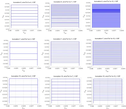
By setting the precision 𝜀 at 10-5 _{and 10}-10_{, respectively, the 5}th_{, 7}th _{and 9}th _order expansions are performed for comparison. The domain splitting on the C20 -C22 plane is shown in Fig.2.

GM =7.7×10−6_km3_/s2_,R

e =3.35km,Tperiod =6.047h

C₂₀ =−9.78×10−2_,C

22 =1.32×10

−2

[C₂₀]=−9.78×10−2_+3σ⋅DA(1) [C₂₂]=1.32×10−2_+3σ⋅DA(2)

8

Figure 2 The domain split on the C20 -C22 plane for a=1.98 at the truncation order of 5, 7 and 10 from the first to the third row, and for each row the error tolerance at 1e-4, 1e-7, 1e-10 from left to right.

9

along which the initial domain is also allowed to split:

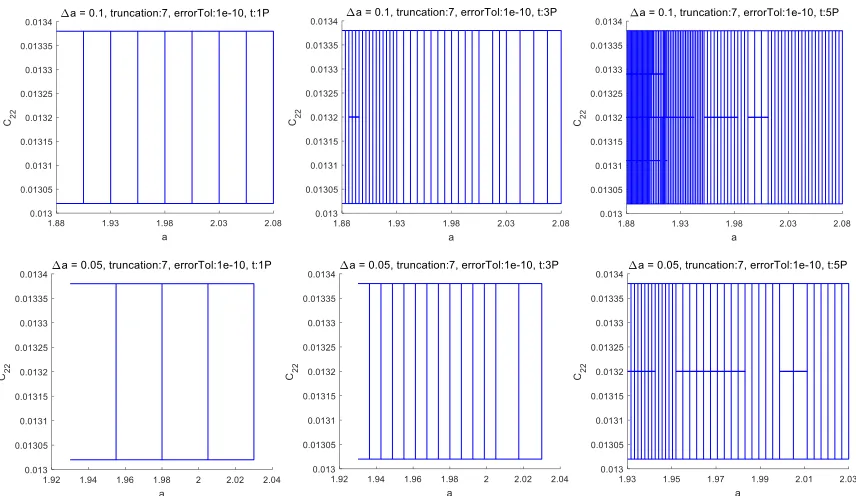
in which a = 1.98 is the semi-major axis of the reference trajectory and ∆𝑎 defines the range of the distance to the asteroid of the orbital motion and is set to 0.1 and 0.05, respectively, in this test. The domain splitting on the a-C22 plane is given in Fig.3.

Figure 3 The domain split on the a -C22 plane for a=1.98 at the truncation order of 7 and the error tolerance at 1e-10.

As shown in Fig.3, if the splitting precision 𝜀 is set at 10-10_{, more splits are needed} for the same truncation order of 7. Further, if the simulation time is increased from one orbital period to two periods, more splits is required along the semi-axis direction, which is still not enough to meet the precision as the first split occurs along the C22 direction. For the same precision, the longer the propagation time is, the more splits of the initial domain occur, due to the accumulation of Taylor expansion error with time and the interaction with highly nonlinear dynamics. In addition, the 9th _order

a=1.98+Δa⋅DA(1)

[C₂₀]=−9.78×10−2_{+3σ ⋅DA(2)} [C₂₂]=1.32×10−2_{+3σ ⋅DA(3)} ⎧

⎨ ⎪

10

truncation does reduce the split efforts as a result of the more accurate approximation of the dynamics, but almost doubles the computation time of the 7th _{order truncation.} Moreover, it can also be seen that the closer the motion to the asteroid is, the more splits are required, which is easy to understand due to the stronger perturbation from the irregular gravity.

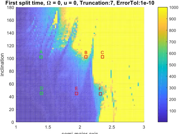
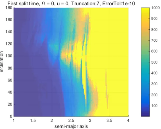
Therefore, for the same error tolerence, the 7th _{order truncation is demonstrated to} better balance the computation time and the accuracy of the splitting process, compared with those of the 9th _{and 5}th _{order truncation, respectively. Therefore, in the} following simulations, the 7th _{order and the error tolerance of 10}-10 _{is applied. In} addition, no split is allowed along the directions of the C20 and C22 term, for the purpose of fully investigating the phase space of the orbital motion. The first split time of the orbits with different geometry is recorded on the semi-major axis and inclination plane, i.e. the a-i plane, which also serves as the sensitivity analysis of the orbital geometry on the uncertainty gravity field. The longer the first split time is, the more stable of the corresponding motion is.

4.

Simulations and Analysis

11

Figure 4 The first split time on the a-i plane with 1-𝜎 uncertainty of 0.63%.

12

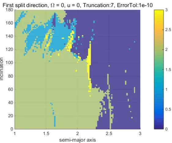
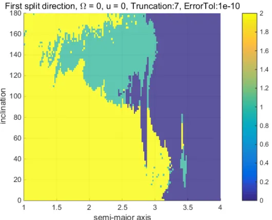
Figure 5 The first split direction on the a-i plane with 1-𝜎 uncertainty of 0.63%.

13

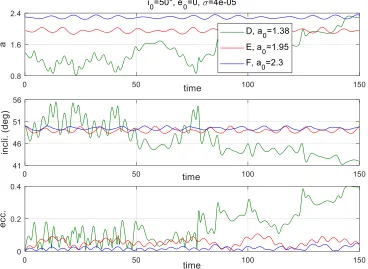
Figure 6 The evolutions of a, e, i of orbits A, B and C in Fig.4.

14

To identify the qualitative effect of uncertainties’ values on the first split time,the 1-𝜎 uncertainties of the C20 and C22 terms are increased from 0.63% to 6.3% in the remaining simulations. Comparing Fig.8 with Fig.4, the blue region extends significantly, meaning that the previous stable motion becomes unstable and the corresponding domain splits, as a result of the larger value of the uncertainty. It can also be seen that the retrograde motion is slightly more stable than the prograde case, which is a phenomenon that is less obvious compared with that of Fig.4. Moreover, around i=110° and a=2.5, there is a yellow region embedded in the blue region, indicating the stability of this region. The structure of Fig.9 coincides with that of Fig.8. The yellow and blue regions of Fig.9 means the first split directions are along the z -axis and x-axis, respectively, which is also in accordance with the previous analysis. In summary, the larger the gravity uncertainty is, the sooner the expansion splits. Resultantly, given the allowed first split time that is determined according to the real mission requirement, practical stable regions can be obtained by identifying whether the expansion splits or not.

15

Figure 9 The first split direction on the a-i plane with 1-𝜎 uncertainty of 6.3%.

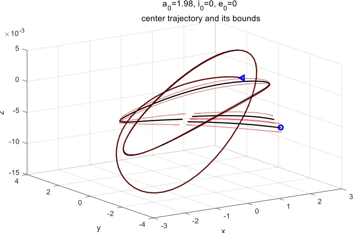
In addition to the first split time, there is the other criterion that indicates the extent of non-linearity, i.e. bounds of the state flow as an evolution of time. The bound is defined as the distance between the lower bound and the upper bound of the flow over the entire uncertainty set. Fig.10 illustrates the evolution, split history and the bounds of a sample orbit with a0=1.98, i0= e0=Ω0=ω0=f0=0. It can be seen that the

16

Figure 10 The evolution of a sample orbit and its splitting history (black lines) and their bounds (red lines)

5.

Conclusions

This study applied ADS to identify the stable and unstable region in the phase space of motion around an asteroid with gravity uncertainty. Asteroid Steins is taken as an example. Firstly, given the accuracy of 10-10_{, the order of Taylor expansion is set to 7,} by compromising between accuracy and efficiency. It is found that the dynamics is more sensitive to the uncertainty on the C22 term, compared with that of the C20 term. Then, the first split time of the orbits with different geometry is obtained on the a-i plane, which highlights abundant dynamical structure. It is found that the closer the motion to the asteroid is the more unstable of the orbital motion is. Moreover, in general the retrograde motion is more stable than the prograde one. This result is validated by the propagating the initial states extracted from different dynamical regions of the first split time plot. In addition to the first split time, the bounds of the state flow are introduced to constrain the evaluation further.

17

dynamical model and real mission requirements should be taken into account.

Appendix

The normalized and non-zero coefficients of the 4th _{order gravity field of Stein [2]}

Stein

C20 -9.78×10-2 C33 -3.55×10-4 C42 -8.55×10-4

C22 1.32×10-2 S31 1.23×10-3 C43 -1.79×10-5

C30 1.37×10-2 S32 -1.08×10-4 S41 -2.03×10-4

C31 1.99×10-3 S33 -1.04×10-3 S42 -1.27×10-4

C32 7.18×10-4 C40 2.52×10-2 S43 -7.64×10-6

- - C41 -2.96×10-4 S44 -1.36×10-5

References

[1] D. Scheeres, Orbital Motion in Strongly Perturbed Environments, Springer, 2012. [2] J. Melman, E. Mooij, R. Noomen, State propagation in an uncertain asteroid gravity field, Acta Astronautica, 91 (2013) 8–19.

[3] A. Wittig, P. Di Lizia, F. Bernelli-Zazzera, R. Armellin, K. Makino, M. Berz, Propagation of Large Uncertainty Sets in Orbital Dynamics by Automatic Domain Splitting, Celestial Mechanics and Dynamical Astronomy, 122(3) (2015) 239-261. [4] M. Berz, Modern Map Methods in Particle Beam Physics, Academic Press, New York, (1999) 82–96.

[5] R. Armellin, P. Di Lizia, F. Bernelli-Zazzera, M. Berz, Asteroid close encounters characterization using differential algebra: the case of Apophis, Celest. Mech. Dyn. Astron., 107(4) (2010) 451-470.

[6] R. Armellin, P. Di Lizia, F. Bernelli-Zazzera, A high order method for orbital conjunctions analysis: sensitivity to initial uncertainties, Advances in Space Research, 53(3) (2014) 490–508.

[7] J. Feng, R. Armellin, X. Hou, Orbit propagation in irregular and uncertain gravity field using differential algebra, Acta Astronautica, 161 (2019) 338-347.

18

under the effects of the C 20 term, the solar radiation pressure and the asteroid's orbital eccentricity, Adv. Space Res. 62 (9) (2018) 2649–2664.

[9] P. Lamy, M. Kaasalainen, S. Lowry, P. Weissman, M. Barucci, J. Carvano, Y. Choi, F. Colas, G. Faury, S. Fornasier, Asteroid 2867 Steins. II. Multi-telescope visible observations, shape reconstruction, and rotational state, Astronomy & Astrophysics, 487 (2008) 1179–1185.