SAMPLE SPACE-TIME COVARIANCE MATRIX ESTIMATION
Connor Delaosa
1, Jennifer Pestana
2, Nicholas J. Goddard
3, Samuel Somasundaram
4, Stephan Weiss
1 1Dept. of Electronic & Electrical Eng., University of Strathclyde, Glasgow, Scotland
2
Dept. of Mathematics & Statistics, University of Strathclyde, Glasgow, Scotland
3DSTL Portsdown, Fareham, Hampshire, UK
4
Thales Underwater Systems, Cheadle, Stockport, UK
ABSTRACT
Estimation errors are incurred when calculating the sample space-time covariance matrix. We formulate the variance of this estimator when operating on a finite sample set, compare it to known results, and demonstrate its precision in simula-tions. The variance of the estimation links directly to previ-ously explored perturbation of the analytic eigenvalues and eigenspaces of a parahermitian cross-spectral density matrix when estimated from finite data.
Index Terms— Space-time covariance, estimation, para-hermitian matrix EVD, polynomial matrices.
1. INTRODUCTION
A parahermitian matrix — typically a cross-spectral density (CSD) matrix emerging as thez-transform of a space-time covariance matrix — can be decomposed into a product of analytic paraunitary matrices and a diagonalised parahermi-tian matrix [1] with few exceptions [2]. A spectrally ma-jorised, not necessarily analytic version of this factorisation is the McWhirter decomposition [3], which approximates the factorisation by polynomial paraunitary and diagonal para-hermitian matrices. A number of algorithms for the latter have emerged [3–10] and in turn triggered various applica-tions ranging from broadband input and multiple-output (MIMO) systems [11, 12], to coding [13], beamform-ing [14, 15], source separation [16] and angle of arrival esti-mation [17, 18], to name but a few.
In applications, the space-time covariance or the CSD ma-trix generally have to be estimated from data. While the accu-racy of the decomposition itself has been investigated in [19, 20], and limiting factors due to algorithm-internal order re-ductions [8, 21–23] and the conditioning of the underlying source model [24] are known, it is only recently that the ef-fect of estimating the space time covariance matrix from a finite data set has been addressed [25]. While [25] linked the
This work was supported in parts by the Engineering and Physical Sciences Research Council (EPSRC) Grant number EP/S000631/1 and the MOD University Defence Research Collaboration in Signal Processing, and a John Anderson Research Award by the University of Strathclyde.
estimation error to the perturbation of the eigenvectors and eigenspaces of the CSD matrix, the formulation of this esti-mation error had still been missing.
This paper aims to close the gap, in order to link eigen-value and -space perturbations directly to the variance of sam-ple space-time covariance. To date, results have been derived for the broadband single channel case, i.e. for the sample auto-correlation sequence. Various attempts have been under-taken for random signals that can be modelled as first order auto-regressive processes [26, 27], or generally [28, 29]. For the broadband case, analysis has generally been restricted to narrowband signals, such that the spatial covariance matrix is Wishart distributed [30, 31]. We derive the variance of a sam-ple cross-correlation sequence, which then forms the building block for the sample space-time covariance. Particularisation of our results agree with [28, 30, 31] and results from spectral estimation such as [32].
We commence with a definition of the space-time covari-ance matrix, and review its properties and matrix factorisation in Sec. 2. In Sec. 3 we analyse the sample cross-correlation sequence, which expands to the space-time covariance in Sec. 4, followed by experimental verification in Sec. 5.
2. SPACE-TIME COVARIANCE MATRIX AND PARAHERMITIAN MATRIX EVD
2.1. Space-Time Covariance
Given M sensor measurements xm[n], m = 1. . . M,
or-ganised in a vector x[n] = [x1[n]. . . xm[n]]
T
, the space-time covariance matrix of the data is defined as R[τ] =
E
x[n]xH[n−τ] , withE{·}the expectation operator. The
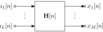
source model or innovation filter [33] in Fig. 1 ties this data vector x[n] to L zero-mean unit-variance mutually inde-pendent complex circularly symmetric Gaussian sourcesu`,
` = 1. . . L, such that E{u`[n]uν[n−τ]} = δ[τ]δ[`−ν]
forν = 1. . . L[34]. As a result, the space-time covariance matrix can be expressed as
R[τ] =X
n
u1[n] x1[n]
uL[n] xM[n]
H[n]
..
[image:2.612.96.262.70.122.2]. ...
Fig. 1. Source model forMconvolutively mixed signals aris-ing fromLindependent unit-variance zero-mean sources.
whereH[n] ∈ CM×L is a matrix of filters. If the entry in
themth row and`th column ofH[n]represents the impulse responsehm`[n], then
rmµ[τ] =
X
n L
X
`=1
hm`[n]h∗µ`[n−τ] (1)
is a cross-correlation sequence that occupies themth row and µth column ofR[τ], with{·}∗denoting complex conjugation.
2.2. Cross-Spectral Density
Since the space-time covariance matrix comprises auto- and cross-correlation sequences, it satisfies the symmetryR[τ] = RH[−τ]. Its z-transform, the cross-spectral density (CSD)
matrixR(z) =P
τR[τ]z−
τ — or shortR(z)•—◦R[τ]to
denote a transfom pair — therefore is a parahermitian matrix, such that its parahermitian transpose, denoted by the operator
{·}P, is equal to itself:RP
(z) =RH(1/z∗) =R(z)[35]. 2.3. Parahermitian Matrix EVD
A parahermitian, analyticR(z)admits a parahermitian matrix EVD (PhEVD) [1]
R(z) =U(z)Λ(z)UP(z), (2) whereU(z)is a paraunitary matrix of eigenvectors andΛ(z)
is a diagonal parahermitian matrix of eigenvalues. In most standard cases, these factors can be selected to be analytic [2]. This is closely related to the McWhirter decomposition [3], where the factorsU(z)and a spectrally majorisedΛ(z)are approximated by polynomials, i.e. are of finite order, while the terms on the r.h.s. of (2) are generally algebraic or tran-scendental.
If the space time covariance matrix is estimated from a finite set of samples, the obtained matrix R[ˆ τ]◦—•Rˆ(z)
will differ from R(z). Similarly, the PhEVD R(ˆ z) = ˆ
U(z) ˆΛ(z) ˆUP(z) will deviate from that in (2). In [25], the
norm of the modelling error
E(z) =R(z)−Rˆ(z) (3) was linked to the deviation in the eigenvalues, i.e. the differ-ence betweenΛ(z)andΛ(ˆ z). The perturbation of the sub-space angle between a particular eigensub-space ofU(z)and of
ˆ
U(z)can in turn be linked to the norm ofE(z)and the dis-tance to the nearest eigenvalue, i.e. near eigenvalues with al-gebraic multiplicity greater than one, subspaces can undergo a larger perturbation [25].
3. SAMPLE CROSS-CORRELATION SEQUENCE
In applications, the space-time covariance matrix must be es-timated from data. If only a set of N snap-shots ofx[n], n = 0. . .(N−1), is available, then generally the estimate for the space-time covariance matrix,R[ˆ τ], will be prone to estimation errors. Since the cross-correlation sequence in (1) is the most general entry of the space-time covariance matrix, we focus on its estimation in order to explore the estimation ofR[τ].
3.1. Unbiased Estimator
The cross-correlation sequence between two signals xm[n]
andxµ[n],m, µ∈ {1. . . M}, is defined as
rmµ[τ] =E
xm[n]x∗µ[n−τ] . (4)
Assuming ergodicity and therefore by implication stationarity for the involved signals, the estimation ofrmµ[τ]over a set of
Ntime snapshots,
ˆ
rmµ[τ] =
1
N−|τ|
N−|τ|−1 P
n=0
xm[n+τ]x∗µ[n], τ≥0
1
N−|τ|
N−|τ|−1 P
n=0
xm[n]x∗µ[n−τ], τ <0
(5)
can be shown to be unbiased. For example forτ≥0, mean{rˆmµ[τ]}=E{rˆmµ[τ]}
= 1
N− |τ| N−τ−1
X
n=0
E
xm[n]x∗µ[n−τ]
= 1
N− |τ| N−τ−1
X
n=0
rmµ[τ] =rmµ[τ],
i.e. the quantity estimated via (5) tends towards the true cross-correlation sequence defined in (4).
3.2. Variance
The variance of the cross-correlation sequence estimator is given by
var{rˆmµ[τ]}=E{(ˆrmµ[τ]−rmµ[τ])(ˆrmµ[τ]−rmµ[τ])∗}
=E ˆ
rmµ[τ]ˆr∗mµ[τ] − E{rˆmµ[τ]}rmµ∗ [τ]− −rmµ[τ]E
ˆ
r∗mµ[τ] +rmµ[τ]r∗mµ[τ]
=E ˆ
Inserting the estimation in (5) into (6), we obtain fourth order terms. For Gaussian signals, the cumulants of order three and above are zero [36, 37], which also holds for the complex-valued case [38], such that
E
xm[n]x∗µ[n−τ]x∗m[n]xµ[n−τ] = E
xm[n]x∗µ[n−τ] · E{x ∗
m[n]xµ[n−τ]}
+E{xm[n]x∗m[n]} · E
x∗µ[n−τ]xµ[n−τ]
+E{xm[n]xµ[n−τ]} · E
x∗µ[n−τ]x∗m[n] . Therefore, forτ ≥ 0, the variance of the estimator in (5) becomes
var{ˆrmµ[τ]}=
1 (N−|τ|)2
N−|τ|−1 X
n,ν=0
E
xm[n+τ]x∗µ[n] · · E{x∗m[ν+τ]xµ[ν]}+
+E{xm[n+τ]x∗m[ν+τ]} E
x∗µ[n]xµ[ν]
+E{xm[n+τ]xµ[ν]} E
x∗µ[n]x∗µ[ν+τ]
−rmµ[τ]r∗mµ[τ]
= 1
(N−|τ|)2
N−|τ|−1 X
n,ν=0
(E{xm[n]x∗m[ν]} · ·E
x∗µ[n]xµ[ν] +
+E{xm[n]xµ[ν−τ]} E
x∗m[ν]x∗µ[n−τ] .
(7) The same result can be obtained forτ < 0, and matches re-sults reached in [32].
Note that the first term in (7) can be simplified as
N−|τ|−1 X
n,ν=0
E{xm[n]x∗m[ν]} E
x∗µ[n]xµ[ν]
=
N−|τ|−1 X
n,ν=0
(E{xm[n]xm∗ [n−(n−ν)]} · · E
x∗µ[n]xµ[n−(n−ν)]
=
N−|τ|−1 X
n,ν=0
rmm[n−ν]rµµ∗ [n−ν]
=
N−|τ|−1 X
t=−N+|τ|+1
(N− |τ| − |t|)rmm[t]rνν∗ [t].
A similar method works for the second term in (7). With
¯
rmµ[τ] = E{xm[n]xµ[n−τ]}denoting the complementary
correlation sequence, the variance of the sample cross-correlation sequence becomes
var{rˆmµ[τ]}=
1 (N−|τ|)2
N−|τ|−1 X
t=−N+|τ|+1
(N− |τ| − |t|)· · rmm[t]rµµ∗ [t] + ¯rmµ[τ+t]¯r∗mµ[τ−t]
. (8)
If u[n] is complex valued with a circularly symmetric dis-tribution, then given the source model in Fig. 1, r¯xy[τ] =
0 ∀τ ∈ Z. Nevertheless, we continue to carry the term in order to particularise the result in (8) to the real valued case.
3.3. Particularisation
The result in (8) generalises a number of solutions reported in the literature. Ifu[n]∈RLandm=µ, then (8) simplifies to
var{rˆmm[τ]}=
1 (N−|τ|)2
N−|τ|−1 X
t=−N+|τ|+1
(N− |τ| − |t|)· · |rmm[t]|2+rmm[τ+t]rmm[τ−t]
. This matches with the result reported in [28].
If the transfer functionH(z)◦—•H[n]is a constant ma-trix,H(z) =H0, then the signalsxm[n]andxµ[n]only have
non-zero correlation for the instant case τ = 0. If further
u[n]∈RLandH0∈RM×L, then the space-time covariance
R[τ] = H0HT0δ[τ]is Wishart-distributed. For the
instanta-neous and real case, (8) simplifies to
var{rˆmµ[0]}=
1
N rmm[0]rµµ[0] +|rmµ[0]|
2
, which indeed matches the variance of a Wishart distribution.
4. SAMPLE SPACE-TIME COVARIANCE
4.1. Sample Space-Time Covariance Error
Assume that the space-time covariance matrix has support of length2τmax+ 1, i.e.R[τ] = 0 ∀|τ| > τmax. Further
as-sume thatR[ˆ τ]is estimated over a support length of2T+ 1. AbbreviatingE[τ] =R[τ]−R[ˆ τ], the mean square error is
ξ=E
( ∞
X
τ=−∞
kE[τ]k2 F
)
=
T
X
τ=−T E
kE[τ]k2 F
| {z }
ξ1
+ 2
τmax X
τ=T+1
kR[τ]k2 F
| {z }
ξ2
,
where the first term,ξ1, is an estimation error due to (8), while
the second term,ξ2, represents a truncation error. Note that
ξ2= 0ifT ≥τmax.
For the estimation error, using (8),
ξ1=
T
X
τ=−T M
X
m,µ=1
var{rˆmµ[τ]}
=
T
X
τ=−T
N−|τ|−1 X
t=−N+|τ|+1
N−|τ|−|t|
(N−|τ|)2 |tr{R[t]} | 2+
+ vec{R[τ−t]}Hvec{R[τ+t]}
-50 -40 -30 -20 -10 0 10 20 30 40 50 -4
-2 0 2 4
-50 -40 -30 -20 -10 0 10 20 30 40 50 0
0.2 0.4 0.6
Fig. 2. (top) ground truth and mean sample cross-correlation sequence, and (bottom) its variance, both calculated accord-ing to (8) and estimated from real valued data.
where the operator vec{·} vectorises its argument andT is the support of the estimate. Therefore, the modelling errorξ depends only on the space-time covariance matrix itself, the sample sizeN, and the support of the estimate,T.
4.2. Optimum Support Length
Note that (9) also presents a formulation for the expected mean square value of the errorE(z)•—◦E[τ]in (3), which forms the basis for the perturbation analysis of the eigenval-ues and eigenvector in [25]. Since the sample sizeN and the specific ground truthR[τ]are given for a particular problem, the only way to minimise this perturbation is the judicious selection of the range of lags,|τ| ≤ T, over whichR[ˆ τ]is evaluated. The optimum valueToptforTin terms of the
min-imum perturbation is therefore Topt= arg min
T ξ .
In general, this will be a trade-off between the termsξ1 and
ξ2. SinceT > τmaxleads toξ2= 0, andξ1generally grows
with increasingT, we findTopt < τmax, i.e. it appears better
to underestimate than to overestimate the support ofR[τ]in practise.
5. SIMULATIONS AND RESULTS
We first demonstrate the accuracy of (8) for the variance of a sample cross-correlation sequence. For an arbitrary given cross-correlation by means of an innovation filter model of order 5 with a single source, L = 1in Fig. 1 and (1), for N= 100the theoretical (8) is compared to the mean variance over an ensemble of size104in Figs. 2 and 3 for a real- and complex-valued scenarios.
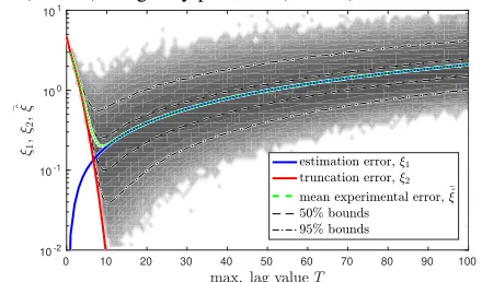
To check the accuracy of the expected estimation error (9), anR[τ]of order 100 is generated by the source model
in [7]. Fig. 4 compares results over an ensemble of104 sam-ple sets, eachL= 500long, to the theoretical values. These match well, and also demonstrate that in this caseTopt = 10
is significantly shorter thanτmax= 50.
6. CONCLUSIONS
This paper has investigated the dependencies of the modelling error that is incurred when estimating a space-time covariance matrix from a finite sample set — this is affected by the size of the set, but also the ground truth space-time covariance ma-trix. The derived expressions match what has previously been identified for sample auto-correlation sequences for the case of temporal correlation only, and to the Wishart distribution in the case of spatial correlation only; in simulations, we have also demonstrated a close match to experiments.
The mean square modelling error is a metric that has pre-viously been established in [25] to perturb the eigenvalues and eigenspaces of the space-time covariance matrix; therefore, the results, particularly (9), now directly link this perturba-tion to the sample size and the ground truth matrix.
-50 -40 -30 -20 -10 0 10 20 30 40 50
-2 0 2 4
-50 -40 -30 -20 -10 0 10 20 30 40 50
-2 0 2 4
-50 -40 -30 -20 -10 0 10 20 30 40 50
[image:4.612.56.298.72.227.2]0 0.2 0.4
Fig. 3. Complex valued equivalent to Fig. 2, with (top) real part, (middle) imaginary part, and (bottom) variance.
0 10 20 30 40 50 60 70 80 90 100 10-2
10-1 100
101
[image:4.612.332.542.337.533.2] [image:4.612.325.545.563.692.2]7. REFERENCES
[1] S. Weiss, J. Pestana, and I.K. Proudler, “On the existence and uniqueness of the eigenvalue decomposition of a parahermi-tian matrix,”IEEE Trans. SP,66(10):2659–2672, May 2018. [2] S. Weiss, J. Pestana, I.K. Proudler, and F.K. Coutts,
“Cor-rection to ”On the uniqueness and existence of the eigenvalue decomposition of a parahermitian matrix”,” IEEE Trans. SP,
66(23): 6325–6327, Dec. 2018.
[3] J.G. McWhirter, P.D. Baxter, T. Cooper, S. Redif, and J. Foster, “An EVD algorithm for para-Hermitian polynomial matrices,” IEEE Trans. SP,55(5):2158–2169, May 2007.
[4] A. Tkacenko, “Approximate eigenvalue decomposition of para-hermitian systems through successive FIR paraunitary transformations,” inIEEE ICASSP, Dallas, TX, Mar. 2010, pp. 4074–4077.
[5] S. Redif, J.G. McWhirter, and S. Weiss, “Design of FIR pa-raunitary filter banks for subband coding using a polynomial eigenvalue decomposition,” IEEE Trans. SP, 59(11):5253– 5264, Nov. 2011.
[6] M. Tohidian, H. Amindavar, and A.M. Reza, “A DFT-based approximate eigenvalue and singular value decomposition of polynomial matrices,” EURASIP J. Adv. Signal Processing,
2013(1), pp. 1–16, 2013.
[7] S. Redif, S. Weiss, and J.G. McWhirter, “Sequential matrix diagonalization algorithms for polynomial EVD of parahermi-tian matrices,”IEEE Trans. SP,63(1):81–89, Jan. 2015. [8] J. Corr, K. Thompson, S. Weiss, I.K. Proudler, and
J.G. McWhirter, “Row-shift corrected truncation of parau-nitary matrices for PEVD algorithms,” inEUSIPCO, Nice, France, Aug. 2015, pp. 849–853.
[9] F.K. Coutts, K. Thompson, S. Weiss, and I.K. Proudler, “A comparison of iterative and DFT-based polynomial matrix eigenvalue decompositions,” in IEEE CAMSAP, Curacao, Dec. 2017.
[10] S. Weiss, I.K. Proudler, F.K. Coutts, and J. Pestana, “Itera-tive approximation of analytic eigenvalues of a parahermitian matrix EVD,” inIEEE ICASSP, Brighton, UK, May 2019. [11] C.H. Ta and S. Weiss, “A jointly optimal precoder and block
decision feedback equaliser design with low redundancy,” in EUSIPCO, Poznan, Poland, Sep. 2007, pp. 489–492. [12] S. Weiss, N. J. Goddard, S. Somasundaram, I. K. Proudler,
and P. A. Naylor, “Identification of broadband source-array responses from sensor second order statistics,” inSSPD, Lon-don, UK, Dec. 2017, pp. 1–5.
[13] S. Weiss, S. Redif, T. Cooper, C. Liu, P. Baxter, and J.G. McWhirter, “Paraunitary oversampled filter bank design for channel coding,”EURASIP J. Adv. SP,2006:1–10, 2006. [14] S. Redif, J.G. McWhirter, P.D. Baxter, and T. Cooper,
“Ro-bust broadband adaptive beamforming via polynomial eigen-values,” inOCEANS, Boston, MA, Sep. 2006.
[15] S. Weiss, S. Bendoukha, A. Alzin, F.K. Coutts, I.K. Proudler, and J.A. Chambers, “MVDR broadband beamforming using polynomial matrix techniques,” inEUSIPCO, Nice, France, Sep. 2015, pp. 839–843.
[16] S. Redif, S. Weiss, and J.G. McWhirter, “Relevance of poly-nomial matrix decompositions to broadband blind signal sep-aration,”Signal Processing,134:76–86, May 2017.
[17] M. Alrmah, S. Weiss, and S. Lambotharan, “An extension of the MUSIC algorithm to broadband scenarios using poly-nomial eigenvalue decomposition,” inEUSIPCO, Barcelona, Spain, Aug. 2011, pp. 629–633.
[18] S. Weiss, M. Alrmah, S. Lambotharan, J.G. McWhirter, and M. Kaveh, “Broadband angle of arrival estimation methods in a polynomial matrix decomposition framework,” inIEEE CAMSAP, Dec. 2013, pp. 109–112.
[19] M.A. Alrmah, J. Corr, A. Alzin, K. Thompson, and S. Weiss, “Polynomial subspace decomposition for broadband angle of arrival estimation,” inSSPD, Edinburgh, Scotland, Sep. 2014. [20] F.K. Coutts, K. Thompson, S. Weiss, and I.K. Proudler, “Im-pact of fast-converging PEVD algorithms on broadband AoA estimation,” inSSPD, London, UK, Dec. 2017.
[21] J. Foster, J.G. McWhirter, and J.A. Chambers, “Limiting the order of polynomial matrices within the SBR2 algorithm,” in IMA Maths in Sig. Proc., Cirencester, UK, Dec. 2006 [22] C.H. Ta and S. Weiss, “Shortening the order of
parauni-tary matrices in SBR2 algorithm,” in ICICSP, Singapore, Dec. 2007.
[23] J. Corr, K. Thompson, S. Weiss, I.K. Proudler, and J.G. McWhirter, “Shortening of paraunitary matrices ob-tained by polynomial eigenvalue decomposition algorithms,” inSSPD, Edinburgh, Scotland, Sep. 2015.
[24] J. Corr, K. Thompson, S. Weiss, I.K. Proudler, and J.G. McWhirter, “Impact of source model matrix conditioning on PEVD algorithms,” inIET/EURASIP ISP, London, UK, Dec. 2015.
[25] C. Delaosa, F.K. Coutts, J. Pestana, and S. Weiss, “Impact of space-time covariance estimation errors on a parahermitian matrix EVD,” inIEEE SAM, Sheffield, UK, July 2018. [26] R.L. Anderson, “Distribution of the serial correlation
coeffi-cient,”Ann. Math. Statist.,13(1):1–13, 1942.
[27] H. Goldsmith, “The exact distributions of the serial correlation coefficients and an evaluation on some approximate distribu-tions,”J. Stat. Comp. and Sim.,5(2,):115–134, 1977. [28] S. Kay, “The effect of sampling rate on autocorrelation
esti-mation,”IEEE Trans. ASSP,29(4):859–867, Aug. 1981. [29] A. Steinhardt and J. Makhoul, “On the autocorrelation of
finite-length sequences,” IEEE Trans. Acoustics, Speech, and Signal Processing, bf 33(6):1516–1520, Dec. 1985.
[30] R.K. Mallik, “The pseudo-Wishart distribution and its appli-cation to MIMO systems,” IEEE Trans. IT, bf 49(10):2761– 2769, Oct. 2003.
[31] L. Zhuang and A.T. Walden, “Sample mean versus sample Fr´echet mean for combining complex Wishart matrices: A sta-tistical study,”IEEE Trans. SP,65(17):4551–4561, Sep. 2017. [32] D.D. Ariananda and G. Leus, “Compressive wideband power spectrum estimation,” IEEE Trans. SP, 60(9):4775–4789, Sep. 2012.
[33] A. Papoulis, Probability, Random Variables, and Stochastic Processes, McGraw-Hill, New York, 3rd edition, 1991. [34] B. Picinbono, “On circularity,” IEEE Trans. Signal
Process-ing,42(12):3473–3482, Dec. 1994.
[35] P.P. Vaidyanathan, Multirate Systems and Filter Banks, Pren-tice Hall, Englewood Cliffs, 1993.
[36] W. B¨ar and F. Dittrich, “Useful formula for moment computa-tion of normal random variables with nonzero means,” IEEE Trans. AC,16(3):263–265, June 1971.
[37] J.M. Mendel, “Tutorial on higher-order statistics (spectra) in signal processing and system theory: theoretical results and some applications,”Proc. IEEE,79(3):278–305, Mar. 1991. [38] P.J. Schreier and L.L. Scharf, Statistical Signal Processing of