Realization of high fidelity power-hardware-in-the-loop capability using a MW-scale motor-generator set

Realization of High Fidelity

Power-Hardware-in-the-Loop Capability Using a

MW-Scale Motor-Generator Set

Qiteng Hong,

Member, IEEE,

Ibrahim Abdulhadi,

Member, IEEE,

Dimitrios Tzelepis,

Member, IEEE,

Andrew Roscoe,

Senior Member, IEEE,

Ben Marshall, and Campbell Booth

Abstract—Power-Hardware-in-the-Loop (PHIL) is a vital technique for realistic testing of prototype systems. While the application of power electronics-based amplifiers to enable PHIL capability has been widely reported, the use of Motor-Generator (MG) sets as the PHIL interfaces has not been fully investigated. This paper presents the realization of the first MW-scale PHIL setup using an MG set as the power amplifier, which offers a promising solution for test-ing novel systems for the integration of distributed energy resources. Uniquely, the paper presents a methodology that introduces augmented frequency and phase control loops that can be integrated to commercially-available MG set’s existing frequency controller for precise frequency and phase tracking. Internal Model Control (IMC) is used for the controllers design and tuning. The developed control algorithm is tested in a MW-scale MG set that couples a GB transmission network model simulated in a real time simulator to an 11 kV distribution network. Experimental re-sults are presented, which demonstrate that the proposed control methodology is highly effective in maintaining the synchronization between the simulated and physical sys-tems, thereby capable of enabling the MG set as a PHIL interface.

Index Terms—Power-Hardware-in-the-Loop (PHIL), con-trol design, real-time systems, power system testing.

NOMENCLATURE

GP Transfer function of the plant being controlled GC Transfer function of the conventional controller Q Transfer function of the IMC controller

e

GP Model of the plant being control

λ Time constant of the augmented low pass filter fref Reference frequency signal

GM G Transfer function of the MG set including its own controller

GO Proprietary controller of the MG set GD MG set’s drive dynamics

GH Inertial response of the MG set

Gm Feedback loop measurement delay in the MG set fM G Frequency of the MG set terminal voltage fe Frequency error in the control loop

GF req Controller of the augmented frequency loop

Q. Hong, I. Abdulhadi, D. Tzelepis and C. Booth are with the University of Strathclyde, UK, e-mail: [email protected]; A. Roscoe is with Siemens Gamesa Renewable Energy, UK; and B. Marshall is with National Grid ESO, UK.

This work is funded by National Grid, UK, under the Network Innova-tion CompetiInnova-tion framework.

fgrid Frequency of the simulated grid voltage Qf IMC controller of the frequency loop

λf Time constant of the augmented low pass filter in the frequency loop

kM G Gain in the MG set’s transfer function

GF Closed-loop transfer function of the frequency loop GF P Transfer function to convert changes in frequency

to changes in phase per second

GP F Transfer function to convert changes in phase per second to the equivalent frequency

GP h Closed-loop transfer function of the phase loop ϕgrid Phase of the simulated grid voltage

ϕM G Phase of the MG set terminal voltage ϕe Phase error in the control loop QP h IMC controller of the phase loop

λph Time constant of the augmented low pass filter in the phase loop

Kf Overall gain of the frequency loop Kph Overall gain of the phase loop

Vgrid Nominal voltage of the simulation grid VM G Nominal voltage of the MG set fn Nominal frequency

H Inertia constant of the MG set KM G

p Proportional control gain of the MG set’s propri-etary frequency controller

K_iM G Integral control gain of the MG set’s proprietary frequency controller

T_dM G MG set drive response time constant TmM G MG set speed measurement time constant KM G

D Damping factor of the MG set

I. INTRODUCTION

economic as the models can be easily changed, extended, and operated under a wide range of scenarios [2].

PHIL has been widely used in the power system domain for various testing purposes [2]–[9]. Particularly in recent years with the increasing demand for integration of distributed energy resource (DER) to the grid, PHIL has become a vital tool to support the development and testing of these resources to de-risk damages to the equipment and also the potential instability to the grid [2]. In [3], a PHIL testbed has been established for testing PV inverter systems; In [4], the PHIL technology is used for testing the performance of various energy storage systems in hybrid electric vehicles; In [5], a 4 MW test bench for evaluating the performance of wind turbines is reported; [6] and [7] present the application of PHIL setups for evaluating novel solutions for frequency regulation using renewable resources; In [8], a PHIL setup is used to emulate the behaviour of variable speed wind turbines; and [9] presents a PHIL platform for islanding detection tests.

The key element for establishing the PHIL capability is the configuration and control of the PHIL interfaces. The most widely used PHIL interfaces include synchronous generators (as reported in this paper and [10], [11]), power converters [12], and linear power amplifiers [13]. In [14], a comparison of these power interfaces for various applications is provided. In [15], [16], algorithms with different reference control and feedback variables for establishing the PHIL interface are com-pared, and the stability issues of PHIL setups are investigated. In [17], a review of the state-of-the-art PHIL techniques is pro-vided, along with discussions of fundamental elements and the associated requirements for establishing PHIL arrangements. These publications provide useful information and guidance for establishing PHIL testbeds, but detailed control of the power interface is not comprehensively discussed. Among the reported PHIL testbeds, the vast majority of the existing work focuses on the use of power-electronics based amplifiers as the PHIL interfaces (e.g. [6]–[9], [12], [13], [18]–[21]), and MW-scale capability has been reported in [13], [19]. While the learnings generated from these publications are significant, the methods are not applicable to PHIL setups with MG sets as the interfaces. There is very limited literature published that has investigated the use of MG sets to enable PHIL, and there is no setup has reported to successfully achieve PHIL using MG sets at a MW scale.

The use of MG set to establish PHIL capability, by na-ture, has fundamental differences from the converter-based interfaces and present unique challenges due to its relatively slower response to command compared to converters. In [10] and [11], the authors attempted to control MG sets to be PHIL interfaces, but the presented control algorithm is only applicable when access to direct control of generator’s input mechanical power is provided. In many cases, particularly for commercially-available MG sets equipped with proprietary frequency controllers, there is a lack of flexibility in the development of control strategy to achieve desired responses. Furthermore, the rating of these reported testbeds are relatively low (around 100 kVA), i.e. the inertia of the machines is small and is relatively fast in responding to commands, so it presents less challenging tasks for the control. The higher

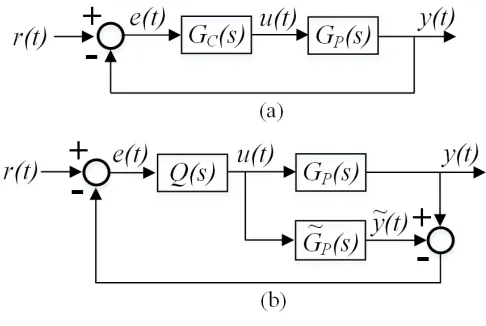
Fig. 1. Typical configuration of (a). Power-Hardware-in-the-Loop (PHIL) setups; (b) Network-in-the-Loop (NiL) setups

rating of the MG set, the more challenging it is to achieve PHIL synchronization due to the larger machine inertia and slower response capability. Therefore, this indeed presents significant technical challenges that have not be resolved and reported by the literature.

This paper presents a novel solution to tackle the aforemen-tioned challenges associated with establishment of MW-scale PHIL testbeds using MG sets. A methodology has been de-veloped, which enables PHIL capability using commercially-available MG sets with proprietary frequency controllers that do not inherently provide adequate responses to frequency commands for the purpose of establishing a PHIL interface. This is achieved by introducing augmented frequency and phase control loops and using the Internal Model Control (IMC) approach [22] for controller design and tuning. The proposed method does not require the change or replacement of the existing proprietary frequency controller, which is unde-sirable and difficult to achieve for commercially-available MG sets. It can be implemented in a separate controller platform, externally to the MG set’s own controller - this avoids the manufactures’ involvements and minimizes the implementa-tion cost. The established testbed couples a GB transmission network model with an 11 kV physical distribution network, and it is the first reported PHIL setup using an MG set that has been successfully achieved at the MW scale, which largely expands the power range that can be tested and offers a promising solution for power system testing.

This paper is structured as follows: Section II and III provide brief introductions of typical PHIL arrangements and the IMC approach respectively; Section IV presents the detailed design and tuning of the augmented frequency and phase controllers for the MG set to enable PHIL capability; Section V presents experimental results to demonstrate the effectiveness of the developed controllers; and Section VI concludes the paper.

II. OVERVIEW OFTYPICALPHIL ARRANGEMENTS

to the real time simulator to close the loop. The PHuT could also be an entire physical network (including generators, loads, cables, etc.), which is shown in Fig. 1.(b). This type of PHIL is also referred as Network-in-the-Loop (NIL) configuration [10], [11]. Both controller devices and power devices can be tested in this arrangement. Controller devices being tested, re-ferred to as Controller Hardware under Test (CHuT), can take measurements from the physical network (and the simulated system if necessary) and apply control actions to the physical network components directly. The effect of the control actions on the physical network is then fed back to the model through the power interface to reflect the changes in the wider network in the simulation. Power devices can also be tested in this arrangement, as the physical network is coupled to the model, which allows a wide range of operational conditions to be emulated and applied to the PHuT to test its reaction to these conditions. This paper will present the control of a MW-scale MG set to enable such an NIL configuration.

III. INTERNALMODELCONTROL(IMC)

The IMC controller [22] is an alternative approach to the Proportional-Integral-Derivative (PID) controller design that has been widely used in industrial applications [23], [24]. Compared to PID controllers, IMC offers, among other ad-vantages, a more straightforward process in terms of design and tuning [25]. This is particularly suitable for developing controllers for systems with high-order behaviors, which is the case for MG sets with proprietary controllers (as demonstrated in Section IV-A).

Fig. 2.(a) shows a conventional feedback control structure. For simplicity of illustrating the concept of IMC, the distur-bance and the measurement delay in the feedback loop are not shown in the figure. The IMC control structure is shown in Fig. 2.(b), where GPe is the model of the plant and Q is

the IMC controller. It should be noted that the conventional and IMC forms of control structures are equivalent and the controllerQandGChave the relationship as described in (1).

GC= Q

1−QGPe

(1)

For the controller design, determiningQinstead ofGC has multiple compelling benefits [25], which include: Q can be determined in a similar way as a feedforward controller, which is more straightforward than designing a feedback controller; the tuning ofQcan be achieved by tuning a single parameter in the augmented low-pass filter (which will be discussed in detail later in this section); and once Q is determined, GC can be subsequently found from using (1) for the actual implementation without losing generality.

In an ideal scenario, where GPe is assumed to be a perfect

model, there will be no feedback loop in the IMC structure, and the ideal controller can be determined directly as Ge−_P1to

achieve “perfect control” [22]. Furthermore, the overall system stability can be guaranteed for a stable controller Qgiven the plant being controlled is also stable.

In practice, it is clear that there will unavoidably be inaccu-racies in the developed model, so the designed IMC controller

Fig. 2. (a). Conventional feedback control structure. (b). IMC control structure

will require further tuning. Furthermore, designing a controller Q = Ge−_P1 is not always realizable. For example, when GPe

contains zeros on the right-hand plane,Ge−_P1will have poles on

the right-hand plane, which will result in an unstable system. To handle this issue associated with system zeros on the right-hand plane, GPe can be represented as:

e

GP =Ge

+

PGe−_P (2)

where Ge

+

P contains all zeros on the right-hand plane while

e

G−_P has all zeros on the left-hand plane. The IMC controller will therefore be designed as (Ge−_P)−1. To handle potential

model and the actual plant mismatch, a low past filter with time constantλis included for tuning the controller. Therefore the ultimate IMC controller can be is expressed in (3):

Q= (Ge−_P)−1

1

(λs+ 1)n (3)

wherenis a parameter used to ensure the overall transfer func-tion is proper. Once Q is found, the conventional controller can be determined using (1). In the following sections, this IMC design approach is used designing the controllers for the augmented frequency and phase loop for enabling MG sets with proprietary frequency controllers as a PHIL interface.

IV. DESIGN OFAUGMENTEDCONTROLLERS TO

ESTABLISHPHIL CAPABILITY

The key objective to control the MG set as a PHIL interface is to ensure its terminal voltage has a high level of synchro-nization with the reference voltage in the targeted bus in the simulated grid. Furthermore, any changes of power flow at the MG set terminal should be effectively fed back and reflected in the simulation.

A. The MG set’s proprietary frequency controller

Fig. 3. Model of the MG set with a proprietary frequency controller

of an example MG set that is used in this work. The transfer function of the MG set with its own controller is:

GM G= GOGDGH

GOGDGHGm+KDM GGH+ 1

(4)

The dynamic performance of the MG set’s proprietary frequency controller in tracking reference signals is reported in [26] and Section V of this paper, which shows that there is significant tracking error during frequency disturbances. Furthermore, there is no mechanism for phase tracking, which is required in a PHIL setup. The control algorithms developed in this paper allow the MG set to enhance the frequency control to achieve precise frequency tracking, while being capable of accurately tracking the reference phase, thereby enabling the MG set to be an effective PHIL interface. It should be noted that, the synchronization between the sim-ulation and the physical network also requires precise voltage magnitude tracking. However, accurate tracking of voltage magnitude can be relatively easily achieved with existing techniques, e.g. solid state excitation systems. According to the studies conducted in [10], the voltage magnitude tracking error can be achieved to the level of 2% for a load step of 0.5 pu. For the purpose of emulating frequency disturbances, the power imbalance is typically smaller than 0.1 pu, so the voltage magnitude tracking does not present significant technical challenges, thus is not the focus of this paper.

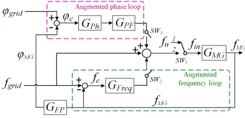
B. Overview of the augmented control structure

A high-level structure of the proposed control scheme for enabling the MG set to operate as a PHIL interface is illustrated in Fig. 4. The augmented frequency control loop enhances the frequency tracking by incorporating an additional feedback loop to the existing frequency controller. The phase control loop further enables the phase tracking by using the phase error to adjust the input frequency signal to the proprietary controller within GM G. During the initialization process, SW1 is at position 1 and both SW2 and SW3 are open so that the machine starts at the nominal frequency; then SW1 will be switched to position 2 so the machine will use simulated frequency as the reference signal; SW2 will then be closed to enable enhanced frequency tracking and SW3 will be closed at the last step to enable phase tracking. The detailed process of initialization of the PHIL simulation will be demonstrated in Section V.

The augmented control loops do not need to access the direct control of input mechanical power to the generator for

Fig. 4. Block diagram of the augmented control for the MG set

frequency tracking (which is required for control algorithms reported in [10], [11]) and does not require the replacement or changing of the MG set’s existing proprietary controller, so it is particularly suitable for establishing PHIL capability using commercially-available MG sets.

C. Design of the augmented frequency controller

When the augmented frequency loop is closed (SW1 at position 2 andSW2closed), the transfer function between the output MG set frequencyfM G and the input reference signal fgrid (i.e. simulated grid frequency) can be expressed as:

fM G=

GM GGF req 1 +GM GGF req

fgrid

| {z }

YR(s)

+ GM G

1 +GM GGF req fgrid

| {z }

YD(s)

(5)

The termYDis equivalent to a disturbance and the objective is to have a controllerGF reqthat can effectively track the input signalfgrid.GM G, as expressed in (6), is the full closed-loop transfer function of the MG set with its proprietary controller. The MG set is equipped with a proprietary PI-type controller, so this has been used as an example to demonstrate the design of the augmented frequency and phase controllers. However, the methodology developed in this paper is also applicable to other types of proprietary controllers.

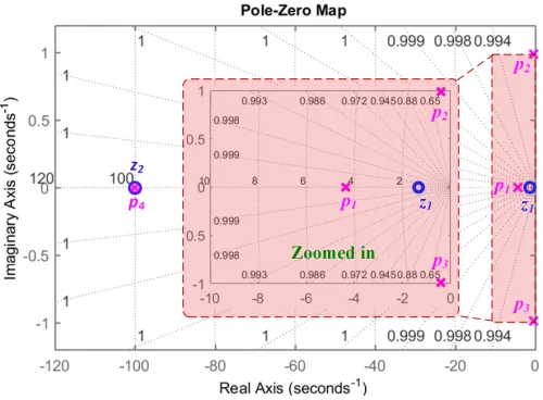
Examining (6), GM G has four poles and two zeros, so it can be represented in a pole-zero form in (7):

GM G=G+_{M G}G−_{M G}= kM G(s+z1)(s+z2) (s+p1)(s+p2)(s+p3)(s+p4)

(7) where G+_{M G} is the part containing all non-minimum phase zeros;kM Gis the gain;G−_{M G}is the rest of the transfer function with all zeros on the left-hand plane;z1andz2 are zeros; and p1,p2,p3andp4are poles. Using the data presented in Table I, the pole and zero map ofGM Gcan be plotted in Fig. 5.

As it can be seen from Fig. 5 that all zeros ofGM G locate on the left hand plane, so G−_{M G} =GM G. Furthermore, one zero (z2) and one pole (p4) are at the same location, which cancel each other out, leading to (8):

G−_{M G}=GM G=

kM G(s+z1)

Fig. 5. Pole and zero map of the MG set model

As discussed in Section III, the IMC controller Qf is the inverse ofG−_{M G}, augmented with a filter to ensure it is proper:

Qf = (s+p1)(s+p2)(s+p3)

kM G(s+z1)(λfs+ 1)nf (9)

where nf is chosen as nf = 2, which ensures the controller to be proper. The resulting controller in the conventional form can then be calculated using (3) and (9):

GF req= Qf 1−GM GQf =

(s+p1)(s+p2)(s+p3)

kM Gλf2s(s+ 2/λf)(s+z1) (10) From the zero and pole map shown in Fig. 5, p1 is a real pole, while p2 andp3 are two complex poles, soGF req can be represented as (11):

GF req=

Gain

z _p}| {

1 2kM Gλfz1×

Low-Pass Filter

z }| {

1 λf

2 s+ 1

×

Lead-Lag Compensator

z }| {

1 p1s+ 1

1 z1s+ 1

×s

2_{+ (p2+p3)s+p2p3}

s

| {z }

PID Type Controller

(11)

It can be seen from (11) that the ultimate controller contains multiple components, i.e. an overall controller gain, a low-pass filter relating to the IMC tuning parameter λf, a lead-lag compensator whose characteristics depend on the pole and zero locations, and a PID type of controller. For simplicity, (11) can be re-written as (12):

GF req=Kf× 1

τf1s+ 1

×τf2s+ 1

τf3s+ 1

×s

2_+a

f1s+af0 s

(12)

where Kf = p1/(2kM Gλfz1), τf1 = λf/2, τf2 = 1/p1, τf3= 1/z1,af1=p2+p3, andaf0=p2p3.

D. Design of the augmented phase controller

The augmented frequency controller (12) will lead to the overall frequency loop behaving as the augmented low pass fil-ter1/(λfs+ 1)nf_{. For the design of the phase loop controller,}

the the equivalent block diagram for the phase loop can be derived and shown in Fig. 6, whereGF is the overall transfer function of the entire frequency loop (i.e. the augmented frequency loop along with the MG set and its own proprietary controller), and the other parameters are introduced in the nomenclature section.

Following the same approach as shown in Section IV-C, the IMC phase controller can be derived as:

QP h=

G−_F1 (λphs+ 1)nph =

(λfs+ 1)2

(λphs+ 1)2 (13)

wherenphhas also be chosen as 2 to makeGP hproper. Using (3) and (13) the phase loop controller can be derived:

GP h= QP h 1−GFQP h

=

Gain

z }| {

1 2λph×

Lead-Lag Compensator

z }| {

λfs+ 1 λph

2 s+ 1

×λfs+ 1

s

| {z } PI Controller

(14)

For simplicity, (14) can be re-written as (15):

GP h=Kph×τph1s+ 1

τph2s+ 1×

aphs+ 1

s (15)

whereKph= 1/(2λph),τph1=λf,τph2=λph/2, andaph= λf.

E. Tuning of the developed controllers

The tuning of the controllers starts from the frequency loop. As mentioned previously, one of the key benefits of the IMC design process is that only one variable, i.e.λf, is involved in turning of the frequency controller. From (12), it can be seen that a smallλf will lead to a relatively large overall gainKf and small time constantτf1. Therefore, if theλf is chosen to be too small, the controller’s response can be too aggressive, resulting in the oscillations or large overshoots of frequency, while if theλfis chosen to be too large, the control action will not be sufficiently effective in tracking frequency. Therefore, during the tuning process, an initial value ofλf can be chosen and then based on the performance of the controller (either too aggressive or too slow) to increase or decease the value of λf accordingly until a satisfactory response is achieved. Similar tuning procedure is used in selectingλphin the phase loop. The ultimate tuned values for all the parameters in the frequency and phase controllers are provided in Table I.

to−180◦, which gives a gain margin of 86.4 dB and 91.6 dB for frequency and phase loop respectively. These reveal the closed-loop system are stable and give reasonably large gain and phase margins. It can also be seen that from Fig. 7 that when the frequency approaches to 0 rad/s, the gain is around 0 dB, which shows the steady state error is approximately 0. The bandwidths of frequency and phase loops’ CLTFs are 4.17 rad/s and 3.52 rad/s respectively.

V. EXPERIMENTALRESULTS

A. Overview of the PHIL setup

The designed control structure, as shown in Fig. 4, and the augmented frequency and phase loop controllers, as described in (12) and (15), have been implemented in the RSCAD software package [27] and run the in the RTS platform from RTDS Technologies [1]. The sampling time of the RTS being used is 50 µs. An overview of the established PHIL configuration is illustrated in Fig. 8. The simulation part of the setup is a GB transmission network model running in real time, while the physical part is an 11 kV distribution network driven by the MG set with a number of load banks connected. The MG set used is consisted of a 1 MW induction motor driving a 5 MVA generator.

The reference frequency fin is generated from the simu-lation and output through the analog output card, which is interfaced with the MG set’s proprietary frequency controller through a fiber. The grid bus in simulation and the MG set bus in physical network are shared buses and the synchronization between two buses is achieved by controlling the MG set terminal voltage (VM G) to be synchronized with the voltage of the grid bus (Vgrid) in simulation.VM GandIM Gare measured and input to simulation through a analogue input card. P-class PMU models [28] provided by the RTS simulation platform [1] are used for measuring the frequency and phase of VM G and Vgrid, which are then fed into the designed augmented frequency and phase controllers as presented in Fig. 4, (12) and (15). Since the same PMU model is used for both simulated and physical network voltage measurement, both quantities will have the same measurement delay, which ensures the comparison is conducted between signals measured at the same time. It should be noted that, while the RTDS simulator is used as the real time simulation platform in this study, other types of real time simulators with equivalent input and output interfaces could also be potentially used for this purpose.

The power exchange between simulation and the physical network is achieved through feeding back the scaled instanta-neous three phase current (ia,ib,ic) from the MG set bus to drive a controllable current source connected to the targeted bus in the model. The total capacity of the load banks in the physical network is 500 kW, but it can be scaled up to a desired level in the simulation through a scaling factor (GI) . The total level of power amplificationGP is:GP = (Vgrid/VM G)×GI.

TABLE I

PARAMETERS OF THEMGSET AND THE TUNED AUGMENTED CONTROLLERS

Parameter Value Parameter Value H 2.7 af1 0.791

KM G

p 4 af0 1.133

KM G

i 5.33 τf1 0.075

TM G

d 0.2 τf2 0.230

TM G

m 0.01 τf3 0.752

KM G

D 1 Kph 2.500

λf 0.150 τph1 0.150

λP h 0.200 τph2 0.100

Kf 2.942 aph 0.150

In the experiments presented in this paper, Vgrid = 400 kV, VM G = 11 kV, and GI = 110. It should be noted thatGI is a configurable scaling factor, and a value of 110 is chosen to ensure a load of 50 kW can be amplified to 200 MW. The value of GI can be chosen to suite different testing needs. As the MG set is only capable of outputting power but not absorbing, therefore, this testbed is most suitable for applications where there is only single-direction power flow is involved.

B. Process of starting the MG set for PHIL simulation

Since the MG set can only be started using its own fre-quency controller, there are a number of steps required during the PHIL start-up process.

1) MG set running purely with its proprietary frequency controller: The MG set is initially commanded to run at the nominal frequency (i.e. fn= 50 Hz) by putting SW1 at position 1 and SW2 and SW3 open as shown in Fig. 4, so that it is at its steady state before being commanded to follow the frequency signal from simulation to avoid undesirable oscillation resulting from the simulation initiation. At this stage, the simulation and the MG set is entirely decoupled. Once the simulation and the MG set have reached their steady states, the input signal fin can be switched to fgrid through SW1 (SW2 andSW3 remain open), where the MG set will purely rely on its own frequency controller to follow the frequency reference signal from the simulation. As mentioned previously, the MG set’s controller is not capable of providing satisfactory frequency tracking during disturbances and there is no phase tracking between the simulation and the MG set.

2) Enabling the augmented frequency loop: When the MG set reaches its steady state with the reference frequency signal from simulation, the augmented frequency loop can be closed by SW2. The results are shown in Fig. 9, where it can be seen that, once the augmented frequency loop is enabled, there is clear improvement in frequency tracking performance with steady state error reduced to below10−3 _Hz.

3) Enabling the augmented phase loop: The phase loop is subsequently closed bySW3, which enables the phase tracking

GM G=

KpM GTmM Gs2+ (KiM GT M G

m +KpM G)s+KiM G 2HTM G

Fig. 6. Equivalent block diagram for the phase loop

Fig. 7. Bode plot of the open-loop and closed-loop transfer function of the frequency and phase loop

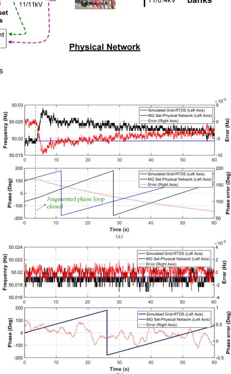
capability. The results are shown in Fig. 10.(a). When the loop is closed, there is a sudden change in MG set frequency in order to adjust the phase. As a result, the phase error starts to decrease from around 100◦. Fig. 10.(b) shows the steady state frequency and phase traces, which shows that with the augmented frequency and phase controllers both enabled, the frequency tracking error is controlled within 10−3 _{Hz, while} the phase error can be maintained below 1◦.

C. Using the testbed for validating a novel frequency response scheme during loss of generation events

In this section, the established PHIL testbed is used for testing a wide-area monitoring and control system, named “Enhanced Frequency Control Capability (EFCC)” [29], for fast frequency response using distributed resources. The EFCC scheme requires relatively complex algorithms and constitutes various distributed control devices and communication links. Any design defects or hardware problems could potentially lead to the deterioration of the control system performance, posing a significant risk of instability to the grid. The PHIL setup, as shown in Fig. 8 and enabled by the proposed control algorithms, provides a realistic test environment for such a system. The PHIL testbed not only allows the validation of the EFCC controllers’ capabilities make correct decisions in con-trolling distributed resources, but also enables the evaluation of the capability of the distributed resources in responding to the control command to provide desired frequency response. In this paper, the EFCC will use measurements from both simulation and physical network for decision making and the distributed resource being used is a load bank emulating

demand side resource, which presents the most challenging scenario for the testbed due to the step change in active power. Fig. 11 shows the frequency tracking performance with and without the augmented controllers during a simulated loss of generation event. The maximum RoCoF during the event is around 0.17 Hz/s. When the MG set purely relies on its proprietary controller for frequency tracking without the augmented control, the maximum error is approximately 0.115 Hz and the average error of 0.0145 Hz. In comparison, with the augmented frequency controller, frequency tracking performance has been significantly improved with a maximum frequency error of 0.025 Hz and an average error of 0.003 Hz. The phase tracking performance is shown in the second plot of Fig. 12 with a maximum error around 10.5◦ and average error of 1.58◦, where with the original controller, there is no phase tracking capability. This performance fulfils the synchronization requirements as specified in [30].

Regarding the EFCC system being tested using the estab-lished testbed, the first plot of Fig. 11 shows the frequency where there is no EFCC scheme enabled and it can be seen that the frequency event leads to a frequency nadir below 49.5 Hz, which is the statuary frequency limit in the GB transmission network [31]. In the second plot of Fig. 11, the EFCC scheme is enabled to provide frequency response from the load banks, which successfully brings the frequency nadir above the required 49.5 Hz limit. Fig. 13 shows the active power at the physical network and the scaled power in the real time simulation. It can be seen that the MG set supplies around 45.2 kW to the load banks, which is amplified as a demand of around 193 MW in the real-time simulated model. At around 5.5 s, the load bank is commanded by the EFCC scheme to reduce its load to 17.5 kW, which is around 27.7 kW load curtailment in the physical network and results in the decrease of around 116 MW load in simulation to provide frequency response. The results shows that the control action to the load bank is successfully reflected to the real time simulated model.

D. Discussion of implementation cost

As any other practical testing platforms, the cost of es-tablishing such a test environment is an important issue to consider. The associated cost of the established PHIL testbed could be classified into two categories: one cost category as-sociated with the physical hardware system and the other cost category relating to the cost of implementing the augmented controllers as presented in the paper.

For the hardware system, it mainly consists of the RTS, the MG set and the physical network. The cost of these three ele-ments can vary significantly depending on the manufacturers, rating of the equipment, the country where they are procured, etc. The actual cost will be subject to the individual setups, so the cost of the specific setup presented in the paper will not be representative.

Fig. 8. Established PHIL testbed using the developed augmented controllers

Fig. 9. Frequency of the simulated grid and physical network - the MG set with the augmented frequency loop enabled

active power of the MG set, which means the manufacturers’ involvement will be required and could potentially be very costly. With the approach presented in the paper, the cost for enabling the PHIL capability is minimal. In this work, the augmented controllers were implemented in RSCAD [27] directly to control the MG set without the need for any changes to the existing proprietary controllers. Therefore, there is no manufacturer involvement required, thus the only additional cost is associated with the engineering time required for the controller implementation.

VI. CONCLUSIONS

This paper has presented the realization of a high-fidelity MW-scale PHIL testbed using a commercially-available MG set with a proprietary frequency controller. Augmented fre-quency and phase controllers have been successfully developed using the IMC approach to enable the MG set as an effective PHIL interface without the need for change or replacement of the MG set’s existing frequency controller. The presented con-trol methodology is tested and demonstrated in an MW-scale MG set, which couples a real-time GB transmission network model with an 11 kV physical network. The established testbed is the first reported PHIL arrangement using a MG set as the PHIL interface at the MW scale, which largely expands the power range that can be tested.

Fig. 10. Frequency and phase of the simulation grid and the physical network: (a) when the phase loop is closed; (b) steady state with frequency and phase loop enabled

Experimental results show that, the developed controllers are highly effective in maintaining synchronization between simulation and the physical system. The PHIL configuration offers a promising solution for power systems prototype testing to de-risk novel technologies (e.g. wide-area control - such as the EFCC scheme) prior to implementation on actual systems.

REFERENCES

Fig. 11. Frequency tracking performance during frequency disturbance

Fig. 12. Phase tracking performance during frequency disturbance

Fig. 13. Power flow in the model and the physical network

[2] DERlab, “European White Book on Real-Time Power-Hardware-in-the-Loop Testing,” Tech. Rep., 2011.

[3] B. Palmintier, B. Lundstrom, et al., “A power hardware-in-the-loop platform with remote distribution circuit cosimulation,”IEEE Trans. on Industrial Electronics, vol. 62, no. 4, pp. 2236–2245, Apr. 2015. [4] R. Trigui, B. Jeanneret, et al., “Performance Comparison of Three

Storage Systems for Mild HEVs Using PHIL Simulation,”IEEE Trans. on Vehicular Technology, vol. 58, no. 8, pp. 3959–3969, Oct. 2009. [5] N. Averous, M. Stieneker, et al., “Development of a 4 MW Full-Size

Wind-Turbine Test Bench,” IEEE Journal of Emerging and Selected Topics in Power Electronics, vol. 5, no. 2, pp. 600–609, Jun. 2017. [6] X. Wang, D. Gao, et al., “Implementations and evaluations of wind

turbine inertial controls with fast and digital real-time simulations,”IEEE Trans. on Energy Conversion, vol. 33, no. 4, pp. 1805–1814, Dec. 2018.

[7] Y. Kim and J. Wang, “Power hardware-in-the-loop simulation study on frequency regulation through direct load control of thermal and electrical energy storage resources,”IEEE Trans. on Smart Grid, vol. 9, no. 4, pp. 2786–2796, Jul. 2018.

[8] F. Huerta, R. Tello, et al., “Real-time power-hardware-in-the-loop imple-mentation of variable-speed wind turbines,”IEEE Trans. on Industrial Electronics, vol. 64, no. 3, pp. 1893–1904, Mar. 2017.

[9] A. Hoke, A. Nelson, et al., “An islanding detection test platform for multi-inverter islands using power hil,”IEEE Trans. on Industrial Electronics, vol. 65, no. 10, pp. 7944–7953, Oct. 2018.

[10] A. Roscoe, I. Elders, J. Hill, and G. Burt, “Integration of a mean-torque diesel engine model into a hardware-in-the-loop shipboard network sim-ulation using lambda tuning,”IET Electrical Systems in Transportation, vol. 1, no. 3, pp. 103–110, Sep. 2011.

[11] A. Roscoe, A. Mackayet et al., “Architecture of a Network-in-the-Loop Environment for Characterizing AC Power-System Behavior,” IEEE Trans. on Industrial Electronics, vol. 57, no. 4, pp. 1245–1253, Apr. 2010.

[12] M. Dargahi, A. Ghosh, P. Davari, and G. Ledwich, “Controlling current and voltage type interfaces in power-hardware-in-the-loop simulations,”

IET Power Electronics, vol. 7, no. 10, pp. 2618–2627, 2014.

[13] M. Steurer, C. Edrington, et al., “A megawatt-scale power hardware-in-the-loop simulation setup for motor drives,”IEEE Trans. on Industrial Electronics, vol. 57, no. 4, pp. 1254–1260, Apr. 2010.

[14] F. Lehfuss, G. Lauss, P. Kotsampopoulos, N. Hatziargyriou, P. Crolla, and A. Roscoe, “Comparison of multiple power amplification types for power hardware-in-the-loop applications,” in 2012 Complexity in Engineering (COMPENG). Proceedings, pp. 1–6, Jun. 2012.

[15] W. Ren, M. Steurer, and T. Baldwin, “Improve the stability and the accu-racy of power hardware-in-the-loop simulation by selecting appropriate interface algorithms,” IEEE Trans. on Industry Applications, vol. 44, no. 4, pp. 1286–1294, Jul. 2008.

[16] N. Marks, W. Kong, and D. Birt, “Stability of a switched mode power amplifier interface for power hardware-in-the-loop,” IEEE Trans. on Industrial Electronics, vol. 65, no. 11, pp. 8445–8454, Nov. 2018. [17] G. Lauss, M. Faruque, et al., “Characteristics and design of power

hardware-in-the-loop simulations for electrical power systems,” IEEE Trans. on Industrial Electronics, vol. 63, no. 1, pp. 406–417, Jan. 2016. [18] K. Jha, S. Mishra, and A. Joshi, “Boost-amplifier-based power-hardware-in-the-loop simulator,”IEEE Trans. on Industrial Electronics, vol. 62, no. 12, pp. 7479–7488, Dec. 2015.

[19] P. Koralewicz, V. Gevorgian, and R. Wallen, “Multi-megawatt-scale fower-hardware-in-the-loop interface for testing ancillary grid services by converter-coupled generation,” in 2017 IEEE 18th Workshop on Control and Modeling for Power Electronics, pp. 1–8, Jul. 2017. [20] B. Lundstrom, B. Palmintier, D. Rowe, J. Ward, and T. Moore,

“Trans-oceanic remote power hardware-in-the-loop: multi-site hardware, inte-grated controller, and electric network co-simulation,”IET Generation, Transmission Distribution, vol. 11, no. 18, pp. 4688–4701, 2017. [21] K. Saito and H. Akagi, “A Power Hardware-in-the-Loop (P-HIL) Test

Bench Using Two Modular Multilevel DSCC Converters for a Syn-chronous Motor Drive,”IEEE Trans. on Industry Applications, vol. 54, no. 5, pp. 4563–4573, Sep. 2018.

[22] D. Rivera, M. Morari, and S. Skogestad, “Internal model control. 4. pid controller design.”Industrial and Engineering Chemistry, Process Design and Development, vol. 25, no. 1, pp. 252–265, 1 1986. [23] B. Kristiansson and B. Lennartson, “Robust tuning of pi and pid

controllers: using derivative action despite sensor noise,”IEEE Control Systems, vol. 26, no. 1, pp. 55–69, Feb. 2006.

[24] B. Lennartson and B. Kristiansson, “Evaluation and tuning of robust pid controllers,” IET Control Theory Applications, vol. 3, no. 3, pp. 294–302, Mar. 2009.

[25] T. Kobaku, S. C. Patwardhan, and V. Agarwal, “Experimental evaluation of internal model control scheme on a dc-dc boost converter exhibit-ing nonminimum phase behavior,”IEEE Trans. on Power Electronics, vol. 32, no. 11, pp. 8880–8891, Nov. 2017.

[26] Q. Hong, I. Abdulhadi, A. Roscoe, and C. Booth, “Application of a MW-scale Motor-Generator Set to Establish Power-Hardware-in-the-Loop Capability,” in2017 IEEE PES ISGT-Europe, Sep. 2017. [27] RTDS Technologies, “Rscad - power system simultaion software,” 2016. [28] “IEEE Std C37.118.1-2011 - IEEE Standard for Synchrophasor

Mea-surements for Power Systems,” 2011.