Data-driven distribution tracking for stochastic non-linear systems via PID design

Data-driven Distribution Tracking for Stochastic

Non-linear Systems via PID Design

Qichun Zhang

School of Engineering and Sustainable Development De Montfort University

Leicester, UK [email protected]

Hong Yue

Department of Electronic and Electrical Engineering University of Strathclyde

Glasgow, UK [email protected]

Abstract—This paper investigates the stochastic distribution tracking problem while the probability density function (PDF) of the stochastic non-linear system output can be controlled to desired distribution. To achieve the control objective, a data-driven approach is proposed in which no information of the system model is required. The output PDF can be estimated by kernel density estimation (KDE) based on the collected system output data. Using the estimated PDF, the probability states can be obtained by sampling operation which can be used to re-characterise the PDF of the system output. Thus, the tracking performance can be achieved by PID control. The parametric selection of the controller has been analysed following the identified PDF dynamic model to assure the convergence of the system output. The effectiveness of the presented algorithm is illustrated by a numerical example.

Index Terms—Stochastic distribution control, non-Gaussian systems, probability density function (PDF), data-driven, PID

I. INTRODUCTION

The stochastic distribution control has been developed for general non-Gaussian systems in late 1990s in which the system output PDF is considered as an extended system output to be controlled [1]. Using the concept of distribution control, the probabilistic decoupling [2], perforamnce enhancement [3], data-based identification [4], non-Gaussian filtering [5], operational control [6] and multipath estimation [7] have been developed recently. Output PDF control is also an important topic for control application e.g. networked DC motor control [8].

The PDF reflects the full information of the stochastic signal in terms of its randomness. To control the shape of the PDF, the relationship between the PDF and the control signal needs to be established. Mostly, there are two approaches to model the dynamics of the system output PDF [9]. 1) Represent of the PDF via neural network modelling. Following this approach, the output PDF is de-composited by the base functions with weighting factors written in a vector, and the dynamics of the weighting vector can be considered as the states of the PDF model [10]. In practice, this approach can be used for paper-making process [11], neural signal transmission [12], [13], etc. The main problem with this approach is that it is numerically demanding to train the neural network weights at each sampling instant, which is difficult for real-time implementation. 2) Establish direct PDF evolution based on

the system model and the known PDF of the noise [14]. Since most models in practice is inaccurate and the PDF of the noise is difficult to obtain, this approach is also inconvenient for implementation. In other words, the existing results based on PDF shaping, for example non-Gaussian filtering and fault diagnosis [15], [16], can be simplified following the presented framework.

To overcome the above-mentioned modelling problems, a question is raised as ’would it be possible to develop the PDF model based on the output data only without using the system model nor the tedious neural network training?’ This is discussed in this paper. In particular, a PDF can be approxi-mated by kernel density estimation (KDE) [17], [18] using the collected system output data. Fixed points can be sampled in the continuous estimated PDF function, through which a group of the associated values can be obtained. These sampled data can be used to form a vector to represent the PDF. Moreover, we can further define this vector as the probability density state (PDS) vector. Following this approach, the PDS vectors of the target PDF and the actual output PDF can be obtained, the distance between them is defined as the error of the PDS vector. The output PDF shaping problem is then formulated as a typical tracking problem for which many control solutions are available. In this paper, the widely used PID design has been adopted due to the simple structure.

The rest of this paper is organised as follows: in Section II, preliminaries and the data-driven modelling have been given including the KDE and PDS representation. The main result on PID control design is presented in Section III. In Section IV, the stability analysis is given. Numerical simulation results and conclusions are discussed in Section V and Section VI.

II. PRELIMINARIES ANDDATA-DRIVENMODELLING

A general SISO stochastic non-linear system can be formu-lated by the following system model:

xk+1=f(xk, uk) +wk

yk=h(xk) +vk (1)

where x ∈ Rn, y ∈ R1 and u ∈ R1 denote the system

state vector, system output and control input, respectively.

w ∈ Rn and v ∈ R1 stand for the random noises with

f :Rn×R1→Rnandh:Rn→R1are non-linear functions.

The following assumptions are made for the system.

Assumption 1. There exist two positive real numbersL1 and

L2, such that the following inequality holds for any sampling instantk.

kf(xk, uk)−f(xk−1, uk−1)k ≤L1k∆xkk+L2k∆ukk Assumption 2. The function h(·) meets Lipschitz condition while there exists a real positive number L3, such that

kh(xk)−h(xk−1)k ≤L3k∆xkk

As the sampled system output values can be collected along

k, such asy1, y2, . . ., the PDF of the system outputy can be estimated by KDE. In particular, we have

ˆ

γk(α) =

1

k k X

i=1

G(α−yi) (2)

whereG(·)denotes the Gaussian kernel function andαstands for the random variable of the system output y and γˆk(α)

approximates the PDF of the system output at each sampling instant k.

The base points in sample space can be pre-specified as

α1, α2, . . . , αm wherem≥n is a positive integer. Thus, the

PDF can be sampled as

zk=

ˆ

γk(α1) ˆγk(α2) . . . ˆγk(αm) T

(3)

where the m-dimensional vector-valued zk is defined as the

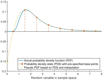
probability density state (PDS). Note thatzk can equivalently

represent ˆγk(α)ifm is selected large enough and the

repre-sentation can be demonstrated by Fig. 1.

0 1 2 3 4 5 6 7 8

Random variable in sample space -0.2 -0.15 -0.1 -0.05 0 0.05 0.1 0.15

Actual probability density function (PDF)

[image:2.612.67.281.471.635.2]

Probability density state (PDS) with pre-specified base points Pseudo PDF based on PDS and interpolation

Fig. 1. PDF representation using probability density states which can be considered as PDF sampling. Note that the interpolation would result in negative parts of the PDF if the base points are scattered along the sample space.

Following the same approach, the target PDFγref can also

be approximated by a m-dimensional vectorzref. Therefore,

the PDF shaping objective can be described by the following objective:

lim

k→∞z˜k →0 (4)

where the error is defined as z˜ = zref −zk. Note that zk

andzref are measurable and all the PDS vectors for sampling

instantk can be obtained using output data only without the system model (1).

Remark 1. Since the PDS can be used to restore the PDF, the base points can be selected following the Shannon’s The-orem which guarantees the sampled PDS maintains enough information. Basically,m≥n.

III. PID CONTROLLERDESIGNALGORITHM

To achieve the control objective, the PID design can be considered as follows:

uk =KPz˜k+KI k X

i=1 ˜

zi+KD(˜zk−z˜k−1) (5)

whereKP ∈Rm,KI ∈Rm andKD∈Rm denote the

pro-portional gain, integral gain and derivative gain, respectively. Although the PID controller parameters can be tuned fol-lowing trial and error method, the parametric selection can be determined by the following systematic design procedure.

Assume that the dynamics of the PDS can be approximately described using the following linear dynamic model.

zk+1=Azk+Buk (6)

where A ∈ Rm×m and B ∈ Rm×1 denote the coefficient

matrices. Then the model in (6) can be rewritten as

zk+1= Θ zkT uk T

(7)

where Θ =

A B

can be identified using least square algorithm sincezi,uiwith∀i < kare known data for sampling

indexk.

The PID control input can be re-expressed using the fol-lowing formula:

uk =K

˜

zT

k p

T

k z˜

T k −z˜

T k−1

T

pk =pk−1+ ˜zk (8)

wherepk = k P

i=1 ˜

zi andK=

KP KI KD .

Denoting z¯ =

z_kT pT_k z_k−T ₁ T

as the extended PDS vector, we have

¯

zk+1= A¯+ ¯BKC¯

¯

zk+

BKP I 0

T zref

zk =

I 0 0 z¯k (9)

whereI denotes the identity matrix and

¯

A=





A 0 0

−I I 0

I 0 0



,B¯ =   B 0 0 

,C¯= 



−I 0 0

0 I 0

−I 0 I 



The gain selection K can be determined by the following theorem.

Theorem 1. There exists a gain matrix K that makes the

dynamics of the PDS-based linear model (6) stable with the extended coefficient matrices (9) and (10), such that the parametric matrix K =W−1_{Y satisfies the following linear} matrix inequality (LMI):

_{−M MA}¯_{+ ¯BYC}¯

MA¯+ ¯BYC¯T

(β−1)M

<0 (11)

where M stands for a symmetric positive definite matrix,

MB¯ = ¯BW and β≥0 denotes the decay rate.

Proof. To ensure the stability of the PID design, the following Lyapunov function candidate can be adopted.

Vk= ¯zkTMz¯k (12)

whereM denotes the real positive definite symmetric matrix

M >0.

Based upon the presented Lyapunov function candidate, we have

Vk+1−Vk = ¯zkT

¯

A+ ¯BKC¯T

M A¯+ ¯BKC¯

−Mz¯k

(13)

We can further consider a decay rate for the Lyapunov function candidate such that the following inequality holds.

Vk+1−Vk≤ −βVk (14)

where0≤β <1.

Then the stability condition can be obtained as follows:

¯

A+ ¯BKC¯TM A¯+ ¯BKC¯−(1−β)M <0 (15) To rewritten the inequality into LMI, we can further in-troduce Y = W K and MB¯ = ¯BW, thus the LMI (11) is obtained using Schur complement and the PID gain can be selected asK=W−1Y which ends the proof.

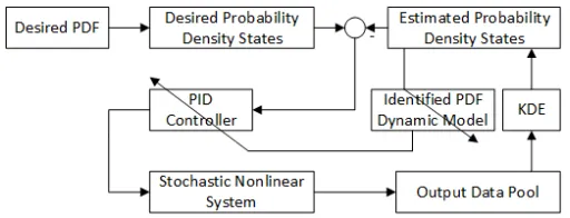
[image:3.612.47.303.585.683.2]

As a summary, the control algorithm can be described by the following block diagram.

Fig. 2. The block diagram of the presented data-driven PDF control via PID.

IV. STABILITY

As the PDF of the system output has been adjusted to the desired PDF, the system output is bounded in mean-value sense. In this section, the stability of the stochastic system output will be analysed without using the result from the system PDF.

Based on the system model (1) and control law (5), the following equations will be obtained.

∆xk+1=f(xk, uk)−f(xk−1, uk−1) +wk−wk−1 (16) and

∆uk= (KP+KD) (˜zk−z˜k−1)−KD(˜zk−1−˜zk−2) +KIz˜k

(17)

where∆xk+1=xk+1−xk and∆uk =uk−uk−1.

Using the assumption of functionf(·)in the system model (1), Eq. (16) results in

k∆xk+1k ≤L1k∆xkk+L2k∆ukk+kwk−wk−1k (18) Note that there always exist two real numberλand¯λsuch that the following inequality holds.

λz˜k ≤z˜k−j−z˜k−j−1≤¯λz˜k, j= 0,1, . . . , k−1 (19)

where λ and λ¯ denote the upper bound and lower bound, respectively.

Thus, Eq. (17) leads to the following result.

k∆ukk ≤ ¯λ(KP +KD)−λKD+KIkz˜kk (20)

As mentioned above, thezk will track the reference with a

non-zero control input, which implies that there always exists a positive real numberσ >¯ 0, such that the following inequality holds

kz˜kk ≤¯σkx˜kk (21)

Applying the mathematical expectation operation to Eq. (18) and substituting Eqs. (20)(21) to Eq. (18), we have

E{k∆xk+1k} ≤ΞE{k∆xkk} (22)

where

Ξ =L1+ ¯σL2 λ¯(KP+KD)−λKD+KI≤1 (23)

sinceE{kwk−wk−1k}= 0.

Based on the assumption of functionh(·), the system output

y is bounded in mean-norm sense once∆xk converge to zero

in mean-norm sense.

To summarise the analysis in this section, a theorem can be given to describe the stability condition of the investigated stochastic system with PDF tracking design.

Proof. The proof of this theorem has been illustrated above.

Following the stability analysis, the pseudo-code has been given to illustrate the procedure of the presented control algorithm implementation where the operation with ∗ means optional step. In other words, the algorithm can also be implemented without ∗steps.

Algorithm 1Data-driven PDF control based on PDS and PID

Require: Data collection of system output y

Input: The desired PDF as the target of the control system

Output: The actual PDF of the system output γ(α)

Initialization: Pre-specified the kernel density function, the dimension ofz, the timetc to replace the pre-control input

by PID controller and the ts for operation time. fork≤ts do

Collect the time sampling data set of y if k≥tc then

Estimate the PDF using the collected datay

Calculate the PDSz for k

Calculate the error of the PDS ˜zfor k

* Identify the model coefficient matricesA andB

* Obtain the PID parameters by solving LMI

uk=P ID else

uk=pre−selectedsignal end if

Update the system with uk k=k+ 1

end for

Restore the output PDF using the final PDS and data interpolation

V. SIMULATION

To evaluate the presented model-free stochastic control al-gorithm, the following numerical example has been considered while the system model is given by

xk+1=xksin (xk+ 0.05)−uk+wk yk= 0.1xk+vk

where process noisewdenotes Gaussian noise with zero mean-value and variance is equal to1. Measurement noisevdenotes Gaussian noise with zero mean-value and variance is equal to 0.1. Due to the non-linearity of the system, the PDF of the system output y is non-Gaussian although the system is subjected to Gaussian noises.

The desired PDF can be pre-specified as Gamma dis-tribution with the parameter a = 1 and b = 2, while the reference zref = [0.005,0.2353,0.1570,0.0027]

with the base points [-5, -1.667, 1.667, 5] in sample space of system output. The PID parameters can be se-lected as KP = diag{1000,1000,1000,1000}, KI = diag{127,127,127,127} andKD= 0. Thus, the simulation

results have been demonstrated by the following figures. Note that the controller will be added into the closed-loop system when k≥100 due to the fact that KDE needs sufficient data to approximate the output PDF. Also, if the PID parameters are determined by the PDS-based dynamic model (6), the sufficient data is also essential to identify the coefficient matrices.

In particular, Fig. 3 demonstrates the PDS zk at k= 1000

and k = 100. Comparing with the desired PDS zref, it has

been show that the PDS zk goes to zref along k while the

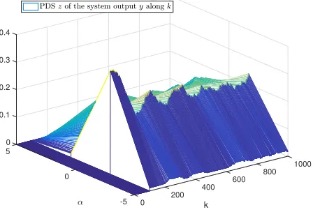
PID control input is given by Fig. 4. The control input is bounded and converges to a constant. To show the complete dynamics of the PDS performance, the 3D mesh for PDS has been indicated by Fig. 5 where zk has been adjusted

dynamically with PID control input. Based on Fig. 5, Fig. 6 show the pseudo PDF of the system outputy. Note that there exist some negative parts which are the errors due to the data interpolation using Matlab. Moreover, the measurable system output is shown by Fig. 7 and it is also bounded using the PID control input which matches the analysis of the stability. The error vectorz˜is illustrated by Fig. 8 which also implies that the PDF tracking is achievable as the errors trend to zero along

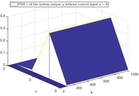
[image:4.612.315.555.498.578.2]

k. In addition, another 3D mesh of the PDSzk is given using

Fig. 9 as a comparison where the control input has been setup asuk= 0and the result shows that the PDF of the investigated

stochastic system output will not be re-shaped without control input.

Based upon the simulation, it has been shown that all the operations are simply to implement without training weights of neural network and PDF evolution. Since the simple control algorithm does not use any information of the system model, we can claim that the presented algorithm is pure data-driven approach sometime we also call it model-free design.

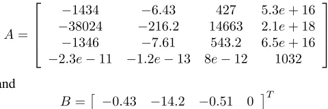
To validate the condition of the PID parametric selection, the identified model can be obtained following the least square method with the collected system output data. The coefficient matrices in Eq. (6) have been estimated as follows:

A=



  

−1434 −6.43 427 5.3e+ 16

−38024 −216.2 14663 2.1e+ 18

−1346 −7.61 543.2 6.5e+ 16

−2.3e−11 −1.2e−13 8e−12 1032



  

and

B =

−0.43 −14.2 −0.51 0 T

which further evaluate the selected PID gain matrices.

VI. CONCLUSIONS

-5 -4 -3 -2 -1 0 1 2 3 4 5 0

[image:5.612.68.280.59.218.2]

0.05 0.1 0.15 0.2 0.25 0.3 0.35 0.4

Fig. 3. The PDSzof the system outputycomparing withk= 100,1000 andzref.

0 100 200 300 400 500 600 700 800 900 1000

k

[image:5.612.322.557.65.217.2]

0 2 4 6 8 10 12 14

Fig. 4. The PID control input for the investigated closed-loop system.

0 5 0.1

1000 0.2

800 0.3

0 ₆₀₀

k

0.4

400 200 -5 0

Fig. 5. The 3D mesh for the PDSzof the system outputywhilezconverges tozref alongk.

[image:5.612.74.282.277.439.2]

data only. Once the fixed base points in sample space have

Fig. 6. The pseudo PDF of the system outputybased on the curve-fitting, PDS and data Interpolation. Note that the PDF should be always positive however the negative part in the figure come from the error of data interpolation

0 100 200 300 400 500 600 700 800 900 1000

k -6

-4 -2 0 2 4 6

Fig. 7. The system outputy of the stochastic system whiley is bounded based on the presented data-driven design.

0 100 200 300 400 500 600 700 800 900 1000 k

-0.15 -0.1 -0.05 0 0.05 0.1 0.15

[image:5.612.330.543.282.447.2] [image:5.612.70.294.495.647.2] [image:5.612.328.543.497.659.2]

0 5 0.1

1000 0.2

800 0.3

0 ₆₀₀

k

0.4

[image:6.612.69.294.64.219.2]

400 200 -5 0

Fig. 9. The PDS of the system outputywithout control input whereu= 0 which shows that the shape of the system output PDF will not be changed alongk.

been pre-specified, the dynamics of the system output PDF is represented by the dynamics of the PDS. Moreover, the target PDF is reformulated by the reference PDS, then the control objective has been transformed equivalently as the distance of the PDS. For the purpose of the practical application, PID design has been used to eliminate the PDS error and the sim-ulation results demonstrate the effectiveness of the presented control algorithm. As a significant component of the control design, the parametric selection of the PID controller has been given following the identified PDS-based dynamic linear model and the stability analysis of the closed-loop stochastic system is obtained. It has been shown that the presented PID -form control input is able to achieve the system output PDF tracking while the system output of the investigated system can be proofed as a bounded stochastic variable. The main contribution of this paper can be summarised as developing a pure data-driven control algorithm for solving the practical probability density function control problem.

ACKNOWLEDGEMENT

This work was supported in part by the HEIF project 2019, De Montfort University, Leicester, UK.

REFERENCES

[1] H. Wang, “Robust control of the output probability density functions for multivariable stochastic systems with guaranteed stability,” IEEE

Transactions on Automatic Control, vol. 44, no. 11, pp. 2103–2107, 1999.

[2] Q. Zhang, J. Zhou, H. Wang, and T. Chai, “Output feedback stabilization for a class of multi-variable bilinear stochastic systems with stochastic coupling attenuation,”IEEE Transactions on Automatic Control, vol. 62, no. 6, pp. 2936–2942, 2017.

[3] Y. Zhou, Q. Zhang, and H. Wang, “Enhanced performance controller design for stochastic systems by adding extra state estimation onto the existing closed loop control,” in2016 UKACC 11th International Conference on Control (CONTROL). IEEE, 2016, pp. 1–6.

[4] Q. Zhang and F. Sepulveda, “Entropy-based axon-to-axon mutual inter-action characterization via iterative learning identification,” inEMBEC & NBC 2017. Springer, 2017, pp. 691–694.

[5] Q. Zhang and X. Yin, “Observer-based parametric decoupling controller design for a class of multi-variable non-linear uncertain systems,”

Systems Science & Control Engineering, vol. 6, no. 1, pp. 258–267, 2018.

[6] Q. Zhang and L. Hu, “Probabilistic decoupling control for stochastic non-linear systems using ekf-based dynamic set-point adjustment,” in

2018 UKACC 12th International Conference on Control (CONTROL). IEEE, 2018, pp. 330–335.

[7] L. Cheng, H. Yue, Y. Xing, and M. Ren, “Multipath estimation based on modifiedε-constrained rank-based differential evolution with minimum error entropy,”IEEE Access, vol. 6, pp. 61 569–61 582, 2018. [8] M. Ren, J. Zhang, M. Jiang, M. Yu, and J. Xu, “Minimum ({h, φ}

)-entropy control for non-gaussian stochastic networked control systems and its application to a networked dc motor control system,” IEEE Transactions on Control Systems Technology, vol. 23, no. 1, pp. 406– 411, 2015.

[9] M. Ren, Q. Zhang, and J. Zhang, “An introductory survey of probability density function control,” Systems Science & Control Engineering, vol. 7, no. 1, pp. 158–170, 2019.

[10] H. Wang,Bounded dynamic stochastic systems: modelling and control. Springer Science & Business Media, 2012.

[11] ——, “Detect unexpected changes of particle size distribution in paper-making white water systems,” IFAC Proceedings Volumes, vol. 31, no. 10, pp. 77–81, 1998.

[12] Q. Zhang and F. Sepulveda, “Modelling and control design for mem-brane potential conduction along nerve fibre using b-spline neural network,” inAdvanced Computational Methods in Life System Modeling and Simulation. Springer, 2017, pp. 53–62.

[13] ——, “Rbfnn-based modelling and analysis for the signal reconstruction of peripheral nerve tissue,” inProceedings of the 8th ACM International Conference on Bioinformatics, Computational Biology, and Health In-formatics. ACM, 2017, pp. 474–479.

[14] L. Guo and H. Wang,Stochastic distribution control system design: a convex optimization approach. Springer Science & Business Media, 2010.

[15] ——, “Fault detection and diagnosis for general stochastic systems using b-spline expansions and nonlinear filters,”IEEE Transactions on Circuits and Systems I: Regular Papers, vol. 52, no. 8, pp. 1644–1652, 2005. [16] L. Yao, J. Qin, H. Wang, and B. Jiang, “Design of new fault diagnosis

and fault tolerant control scheme for non-gaussian singular stochastic distribution systems,”Automatica, vol. 48, no. 9, pp. 2305–2313, 2012. [17] J. Zhang, S. Zhou, M. Ren, and H. Yue, “Adaptive neural network cascade control system with entropy-based design,”IET Control Theory & Applications, vol. 10, no. 10, pp. 1151–1160, 2016.