Studies of Gas Absorption In Infrared Spectra of Carbon-Rich AGB Stars

(1)

Theses Thesis/Dissertation Collections

5-20-2015

Studies of Gas Absorption In Infrared Spectra of

Carbon-Rich AGB Stars

Xingchao Yu

Follow this and additional works at:http://scholarworks.rit.edu/theses

This Thesis is brought to you for free and open access by the Thesis/Dissertation Collections at RIT Scholar Works. It has been accepted for inclusion in Theses by an authorized administrator of RIT Scholar Works. For more information, please contactritscholarworks@rit.edu.

Recommended Citation

(2)

R

•

I

•

T

Studies of Gas Absorption In Infrared Spectra of Carbon-Rich

AGB Stars

by

Xingchao Yu

A Thesis Submitted in Partial Fulfillment of the

Requirements for the Degree of Master of Science in

Imaging Science

Chester F. Carlson Center for Imaging Science

College of Science

Rochester Institute of Technology

Rochester, NY

May 20, 2015

Signature of the Author__________________________________________

Accepted by___________________________________________________

(3)

CHESTER F. CARLSON CENTER FOR IMAGING SCIENCE

COLLEGE OF SCIENCE

ROCHESTER INSTITUTE OF TECHNOLOGY

ROCHESTER, NEW YORK

CERTIFICATE OF APPROVAL

MASTER OF SCIENCE DEGREE THESIS

The M.S. Degree Thesis of Xingchao Yu has been examined and approved by the

thesis committee as satisfactory for the thesis required for the

Master of Science degree in Imaging Science

______________________________________

Dr. Joel H. Kastner, Thesis Advisor Date

______________________________________

Dr. Benjamin Sargent, Thesis Advisor Date

(4)

Studies of Gas Absorption In Infrared Spectra of Carbon-Rich

AGB Stars

by

Xingchao Yu

Submitted to the

Chester F. Carlson Center for Imaging Science in partial fulfillment of the requirements

for the Master of Science Degree at the Rochester Institute of Technology

Abstract

An asymptotic giant branch (AGB) star is a dying, Sun-like star, and it is actively expelling its mass into an envelope around the star, forming a circumstellar shell. Infrared spectra can reveal the composition of the material within this shell, informing studies of the recycling of the products of stellar nuclear processing in the Universe. In this study, we want to identify how the differing metallicities of our own, relatively metal-rich Milky Way galaxy and the nearby, lower metallicity Large Magellanic Cloud (LMC) galaxy affect gas composition in the circumstellar shells of carbon-rich AGB stars.

(5)

LMC) and to spectra obtained using the Short Wavelength Spectrometer (SWS) on board the Infrared Space Observatory (ISO; for the Milky Way), we determine basic physical characteristics, such as gas temperature and shell radius, for each star, as well as the relative amounts of gas species for each star, by matching models to the observed spectra.

(6)

Acknowledgements

First and foremost, I express my sincerest gratitude to both of my thesis advisors, Dr. Joel H. Kastner and Dr. Benjamin Sargent, who have supported me throughout my thesis with constant encouragement, guidance and understanding. I am grateful for having good advisors.

I would like to express my deepest appreciation for the huge amount of help, support and patience from Dr. Benjamin Sargent. Without Ben’s selfless dedication and collaboration, this thesis would not have been possible. I gratefully thank Ben for his assistance with the IDL code for the model and other contributions including his previous work related to this research. His timely support, constructive comments, and substantial suggestions dramatically helped and advanced the completion of this thesis.

I would like to thank my advisor Dr. Joel Kastner again especially for providing me the opportunity to this research project. And it is him who encouraged me to work with Ben, and thanks to him, the collaboration between Ben and me is possible.

I would also like to thank my thesis committee member Dr. John Kerekes for providing me with invaluable guidance and advice during the process.

I would like to thank Dr. Gregory C. Sloan as well, who originally suggested this project and provided informational data and insightful suggestions.

(7)

Chapter 1

Introduction

1.1 Background of AGB Stars: Stellar Evolution

(11)

First, there is a giant molecular cloud of gas and dust in the interstellar medium prior to any star’s formation. Due to gravitational forces, an over-dense clump of this cloud of gas and dust will begin to contract to form a protostar.

As the cloud clump contracts, the gravitational potential energy is converted to thermal and radiative energy. So the contracting cloud clump becomes hotter and hotter, and when its core heats up to the ignition temperature for fusion reactions, then a star is born (the start of the main sequence). A main sequence star will stably burn its hydrogen in its core and thus stay relatively in the same point on the H-R diagram for a long period.

Before that, the contracting cloud is called a protostar before hydrostatic equilibrium is established. And after hydrostatic equilibrium starts but before the fusion ignition, it is called a pre-main sequence star (PMS). The track traced on the H-R diagram before main sequence is called a PMS evolutionary track.

AGB stars are formed in the post main sequence stages when the core finishes its fusion burning. Both hydrogen and helium are depleted in the core, while mostly carbon remains inside. Fusion continues to burn in the layer around the core. During this stage, the star loses much of its mass, which dissipates into interstellar medium. The whole process of stellar evolution, including the AGB stage, will be discussed more below.

1.1.1 Protostar and Pre-Main Sequence

(12)

pre-main-sequence (PMS) star. The protostar later becomes visible to us, either by accreting or dissipating the surrounding materials. A PMS star shines by slowly shrinking and accreting. The total time from the start of collapse and to the end of PMS is only on the order of a few million years (in the case of a solar mass star, about 20 million years).

The PMS star has a lower surface temperature than it will have on the main sequence, and its radius is much larger, but overall it still has a higher luminosity than it will have on the main sequence. Because the star’s temperature is very low, the energy is transported outward within the star by convection rather than radiation. The star is larger than it will be on the main sequence and the larger surface area gives rise to the higher luminosity. That is why the luminosity during PMS is much higher than it will be in the main sequence. The central temperature increases as the PMS star evolves, but the surface temperature does not change very much. As the star shrinks in size, so the luminosity decreases. So the point on a H-R diagram moves downward during the PMS phase. As the core temperature continues to heat up, the opacity decreases, and eventually the transport of the energy in the core becomes effectively due to radiation rather than convection. Finally, the core heats up to a few million Kelvins, and the thermonuclear reactions are ignited. When the PMS star gets most of its energy from thermonuclear reactions rather than gravitational contraction, the star is now called a ZAMS (zero-age main-sequence) star. The heat from the fusion reaction keeps the star in hydrostatic equilibrium now instead of the heat created by gravitational collapse.

1.1.2 Main Sequence

(13)

As mentioned earlier, main-sequence stars are in hydrostatic equilibrium, where outward thermal pressure created from the heat of nuclear fusion in the hot core is balanced by the inward pull. The energy is transported by radiation and convection, the amounts depending on the mass and age of the star. In a convection zone, the energy is transported by bulk movement of plasma with hotter material rising and cooler material descending.

There are two ways to convert hydrogen to helium: one is through the PP chain, (proton-proton chain, which directly fuses hydrogen together in a series of stages to produce helium.) There are three types of PP reaction chains. The other is the CNO cycle, and this process requires a carbon nucleus as a catalyst, and it uses atoms of carbon, nitrogen and oxygen as intermediaries in the process of fusing hydrogen into helium (Clayton, 1983). Thus, main sequence stars can employ two types of hydrogen fusion processes. Astronomers divide the main sequence into upper and lower parts, based on which of the two is the dominant fusion process. In the lower main sequence (low mass star), energy is primarily generated as the result of the PP chain. Stars in the upper main sequence (higher mass stars) have sufficiently high core temperatures to use the CNO cycle efficiently. At stellar core temperatures of 18 million Kelvin, the PP process and CNO cycle are equally efficient (Clayton, 1983).

(14)

The observed upper limit for a main-sequence star is 120–200 solar mass (Oey & Clarke 2005). Stars above this mass cannot radiate energy fast enough to remain stable.

The lower limit is 0.08 M☉. This is the lower limit for sustained proton–proton nuclear

fusion (Karttunen et al. 2007).

Although more massive stars have more fuel to burn, they also must radiate a proportionately greater amount with increased mass, so they burn faster. As a result, the more massive the star, the shorter its life time on the main sequence (Zeilik & Gregory 1998). The most massive stars may remain on the main sequence for only a few million years, while stars with less than a tenth of a solar mass may last for over a trillion years (Laughlin et al. 1997). After the hydrogen fuel at the core has been consumed, the star evolves away from the main sequence on the HR diagram.

1.1.3 Post-Main Sequence

After the main sequence phase, The behavior of a star now depends on its mass, with a star much below a solar mass but Above 0.08 solar masses (for a mass of material less than 0.08 solar masses, it is called a brown dwarf), while a star with up to 10 solar masses passes through a red giant stage (Bahcall et al. 2001). A more massive star can explode as a supernova (Barnes et al. 1982), or collapse directly into a black hole.

Solar Mass Star

(15)

Although the thermonuclear reactions dwindle in the core, they continue in a shell around the core. The radius of the star grows. As a result, the surface temperature decreases. The opacity increases, and the convection carries most of the energy outward in the star. As the radius increases, then luminosity increases greatly. Now the star enters into red giant branch (RGB) phase, since it has shifted to the red as temperature decreases and it becomes bigger and brighter. On the H-R diagram, the RGB phase begins after moving rightwards to lower temperatures from the main sequence and upwards to higher luminosities.

An RGB star is different inside from a main sequence star. Its core is highly mass condensed and extremely hot, so that the gas inside becomes degenerate and produces degenerate gas pressure, which enables the core to balance its own gravitational force. So now it is quantum mechanical pressure instead of thermal pressure keeping the star in hydrostatic equilibrium.

(16)

The star now has changed to a new equilibrium state, switching from the red giant branch to the horizontal branch of the H-R diagram. This is an analog of the star’s main sequence, since the fusion burning is stable again. This horizontal branch term is so-named because the luminosity of the star will stay relatively stable during the stage, while its surface temperature increases and then decreases, migrating horizontally across the H– R diagram (Karttunen et al. 2007).

Eventually, the helium fusion converts the core to carbon. Then the reactions in the core stop, but moves onto the layer around it. This stage is very similar to when the hydrogen has been used up in the core at the end of main sequence. This same physical process makes the star expand and move off the horizontal branch and become a red giant again! Only this time, we call it an asymptotic giant branch (AGB) star on the H-R diagram. (The AGB phase will be discussed more in the next Section.) And the electrons in the core become degenerate again.

After the AGB stage, for a star of roughly a solar mass or less, carbon burning can never happen because the core is degenerate and cannot contract and heat to the carbon fusion ignition point. After about 75,000 years, the star becomes a white dwarf, mostly carbon, with no energy source, and it gradually cools afterwards.

Intermediate-Mass Star

For a star a little heavier than the Sun, say, 5 solar masses, the very center of the core has a temperature high enough to initiate the CNO cycle (more than 15 million K) at the beginning of the main sequence.

(17)

heats up rapidly. Meanwhile, the outer envelope expands, and the surface temperature of the star gets lower. It moves to the right on the H-R diagram.

During the very end of the expansion, convection develops so luminosity increases instead of decreases. At this point, the RGB phase begins. The core continues to heat up, and, finally, helium start to burn. But helium burning is very short this time. So no helium flash in this case. When the burning ends, the gravitational contraction takes over again until it reignites the helium burning. Then the helium burning in the core gradually becomes dominant instead of the hydrogen burning in the shell. The star becomes hotter, and moves to the left on the H-R diagram. When the helium is exhausted in the core, the contraction begins again. This whole process traces a path on the H-R diagram similar to the horizontal branch, but it is not the same. Similar to a solar mass star, the evolutionary track turns into AGB when a helium burning shell around the core is formed. Next, it becomes a white dwarf, sending mass into interstellar medium.

High Mass and Low Mass Star

For a high mass star, say 25 M☉, its evolutionary track after the main sequence

becomes almost horizontal on the H-R diagram, and a much shorter life time brings it quickly to the red supergiant phase. Soon, the core becomes unstable and collapses, causing the star to end in a supernova explosion.

For a star with over 50 solar masses, the mass loss by stellar winds changes its

evolutionary track dramatically. The Sun’s mass loss rate is about 10-14 M☉per year, due

to the solar wind. Asymptotic giant branch and red supergiant stars lose their mass at

rates of 10-7 to 10-4 M☉ per year (Chiosi & Maeder 1986). By the end of its main

(18)

Stars with mass much lower than that of the sun also have significantly different

evolution tracks. Red giants with 0.08 to 0.2 M☉ slowly burn hydrogen for trillions of

years, becoming “blue dwarfs”, then white dwarfs (Laughlin et al. 1997). Objects with

mass less than 0.08 M☉ do not even reach main sequence. Before it can heat up to

ignition point of fusion reactions, the core density is already high enough to form degenerate matter. The degenerate gas pressure directly counterbalances contraction. The star simply cools off as a brown dwarf.

As we can see, AGB stars mostly evolve from low to intermediate mass stars.

1.1.4 Asymptotic Giant Branch Stars

As mentioned above, a star enters the AGB stage when the core runs out of helium (and consists mostly of carbon and oxygen). A helium burning shell is formed around the core and is the main energy source. Fusion of hydrogen still continues, but in an outer thin shell. The star's radius increases. Since the helium fusion reaction (triple-alpha) is very sensitive to temperature, the AGB star becomes very unstable when the helium shell is running out of fuel. The hydrogen fusion in the outer thin shell dumps helium onto the inner helium shell. Eventually, the helium shell ignites explosively, a process known as a helium shell flash. The shell flash forces the star to expand, and the expansion cools down the hydrogen-burning shell, which causes the hydrogen burning to cease temporarily. The helium shell runs out of fuel, the star contracts, the increased temperature reignites hydrogen fusion, and the cycle begins again. This whole phase is called a thermal pulse.

(19)

the final stages of a star’s life. Though not well understood yet, the mass loss is believed to happen as follows. Stellar pulsations lift stellar material and cool it to the point that dust grains can condense. The dust experiences radiation pressure from stellar radiation and is pushed away from the AGB star. The dust grains push on the gas molecules in the lifted stellar material, “shepherding” the stellar gas along with them in a great mass outflow. AGB stars evolve further into short-lived preplanetary nebulae. The final fate of an AGB envelope is to become planetary nebulae. A star may lose its 50% to 70% of its mass during the AGB phase. AGB stars are believed to be one of the main types of dust-producing sources in galaxies.

(20)

1.2 Literature Review on Studies of C-Rich AGB Stars

(21)

Leisenring et al. (2008) explain this phenomenon using the effect of dust dilution. Only when C2H2 absorption overcomes the effects of dust dilution because of its increasing density, the equivalent width will grow higher. The behavior above shows that the dust dilution affects the 13.7-µm C2H2 Q branch at low mass-loss rates, whereas the effects of dust veiling on the P and R branches at 7.5 µm are more important at higher mass-loss rates. The higher mass-loss rate has a less effect on sources in the Magellanic Clouds compared to the Milky Way, indicating less dust dilution at lower metallicities. This metallicity dependence is not observed for the Q branch. This confirms the previous results from Matsuura et al. (2006) that the 13.7-µm C2H2 absorption band must originate throughout the circumstellar dust shell, whereas the 7.5-µm absorption band, which only has P and R branches transitions, originates at depths below those favoring Q-branch transitions, closer to the inner regions of the circumstellar envelope.

Zijlstra et al. (2006) also studied carbon stars observed using Spitzer-IRS,but they focused more on dust emission bands (SiC, MgS). They investigate the strength and central wavelength of the SiC and MgS dust bands as a function of spectroscopic color and metallicity. But as for gas absorption, they find that the circumstellar 7.5-µm C2H2 band is found to be stronger at lower metallicity, explained by higher C/O ratios at low metallicity. Similar to Leisenring et al., they also found the dust veiling is stronger then the gas absorption for the 13.7-µm feature when the mass loss rate is low. It has a stronger dependence on the gas density than the dust column density at higher gas mass loss rates. The narrow 13.7-µm Q branch is prominent in almost all spectra. It arises from C2H2 ν5 transition (Tsuji 1984; Aoki et al. 1999; Cernicharo et al. 1999). According to

(22)

Similar to Leisenring et al (2008), Zijlstra et al. (2006) also mention that the 11.3 µm SiC emission feature affects the absorption band and makes it difficult to judge how strong and broad the P and R branches are. The 14.3-µm HCN (Hydrogen Cyanide) band in Galactic carbon stars reported by Aoki et al. (1999) and Cernicharo et al. (1999) is either weakly present or not present in the spectra in their LMC samples. But they are noticeably present in the 7.5-µm feature. This agrees with Matsuura et al. (2002, 2005), who mention that, at low metallicity, HCN is less abundant relative to C2H2. Galactic carbon stars have absorption in this wavelength region from C2H2, HCN, and CS (Carbon Sulfide; Goebel et al. 1981; Aoki et al. 1998). They also note the existence of another 5 µm absorption band that is usually very strong, and is caused by CO and C3 (Jørgensen et

al. 2000), and it extends beyond the blue limit of the wavelength range. This explains the sharpness of the blue edge of the spectra.

Another paper that investigates the molecular bands in carbon-rich AGB stars in the LMC using the Spitzer-IRS data is Matsuura et al. (2006). They use Gaussian fitting instead of measuring the equivalent width to represent band strength. Similarly, they found the HCN bands at 7.5 and 13.7 µm to be very weak or absent compared to C2H2, and they found no clear difference in the C2H2 abundances among LMC and Galactic stars. They found the gas mass-loss rates in their stars to be in the range 3 × 10-6 to 5 ×

10-5 M

☉yr-1 from column densities obtained by fitting models to the 13.7-µm absorption

(23)

C2H2 at 500 K. This suggests that these molecular bands are indeed of circumstellar origin.

Aoki et al. (1999) stress the importance of analyzing the 14-µm HCN and C2H2 absorption features over the other spectral features. They also detected HCN bands excited by radiative pumping in TX Psc and V CrB (two AGB stars), proving that HCN can exist in the circumstellar shell. Except for TX Psc, they also confirm that the 13.7-µm Q band appears in all the stars in their study (4 optical carbon stars and 4 candidates of infrared carbon stars by ISO SWS) along with the broader P and R branches, which arise in the warmer envelope close to the star. Aoki et al. use different line lists, which they created by themselves instead of using the HITRAN line list (Rothman et al. 2009 for HCN, Rothman et al. 2013 for C2H2 and CS). From their line list, they found that, when the temperature of the gas increased to 1000 K, the general shape of the Q branch in the 14 µm would be significantly affected, while the P and R branches are less affected. In their results, when the gas temperature is low, there is a smaller minor absorption feature long-ward of 13.7 µm in addition to the main 13.7-µm feature. These merge together when the temperature reaches 1000 K. They find the Q branch in the observed spectrum is much weaker compared to the synthetic one. The weakness could possibly be explained by the dilution of the absorption by dust emission, but they also admit that this would not completely explain the total weakness of the Q branch in the observed spectrum.

(24)

(25)

1.3 Summary and Main Purpose of This Research

From the papers discussed above, we know that C2H2 is present in all the carbon stars. Matellicity plays a role in the circumstellar shell formation. Dust dilution will affect the P, R and Q branches. Also, effective temperature and other physical parameters will affect the gas bands, too. In addition, the 7.5-µm and 14-µm absorption bands, especially from C2H2, arise from different depths in the circmstellar envelope. There are also dust emission features that will affect the overall spectral appearance.

(26)

Chapter 2

Observations and Data

2.1 Spitzer Space Telescope Observations and Data Reduction

2.1.1 Spitzer Telescope and IRS Instrument

The Spitzer Space Telescope, NASA’s Great Observatory for infrared astronomy,

(27)

Spitzer utilizes an Earth-trailing solar orbit, meaning that it follows a solar orbit, but trailing the Earth (Werner et al. 2004). This offers two major advantages over an Earth’s orbit: separation from the Earth’s thermal radiation and from the particles in its Van Allen radiation belts. First, this makes sure the telescope is away from the radiation from the Earth, which enhances the telescope’s radiative cooling. This also ensures the solar array can always pointed at the sun while the other side of the telescope can always face dark space, with no heat interfering. The absence of eclipses makes for a stable thermal configuration and reduces the variability of alignment, permitting excellent sky views and observing efficiency. Second, the solar orbit is not affected by the charged particles in the Earth’s Van Allen radiation belts. The particles will destroy the infrared spectrum detectors, causing bad pixels on the detector.

Spitzer has three instruments built in (Werner et al. 2004): the Infrared Array

Camera (IRAC), the Infrared Spectrograph (IRS), and the Multiband Imaging Photometer (MIPS). Both IRAC and MIPS are primarily photometry detectors while MIPS does have limited spectroscopic ability. The IRS is the spectral detector that observed half of the targets in our study. There are no moving parts in the entire instrument payload except for a scan mirror in the MIPS (Werner et al. 2004).

(28)

𝜃 =1.22 _𝐷𝜆. (2.1)

The slit width covers two pixels on its detector. But the pixel size is different for different modules according to the differing spatial resolution for different arrays. Also, both low-resolution modules contain two sub-slits, one for the first order spectrum and one for the second-order. These two sub-slits further divide the two wavelength ranges into four wavelength sub-ranges: 5.2 to 7.7 µm , 7.4 to 14.5 µm, 13.3 to 18.7 µm and 18.5 to 26.0 µm (Houck et al. 2004). When using the second order sub-slit to capture a source, there will be also a “bonus” order caused by the appearance of a short piece of first order on the array that is allowed through the second order sub-slit. It improves the overlap between the first and second order. The high-resolution modules have 10 orders, 11th to 20th, falling on their arrays (Houck et al. 2004),

Both short wavelength modules utilize Si:As detectors that have 128 × 128 pixels, while both long wavelength modules use Si:Sb detectors with the same number of pixels (Houck et al. 2004). The Si:As detectors are less vulnerable to pixel damages, while the longer wavelength detectors have more dead pixels. The low-resolution modules have long slits and are designed for optimum sensitivity to dust absorption features while the two high-resolution modules are optimized for emission lines. The high-resolution models are designed to achieve the highest possible resolutions, near 600 in spectral resolution (calculated by λ/dλ, where dλ is the resolution element), while the low-resolution model have spectral low-resolution ranging from 64 to 128 (Houck et al. 2004). Usually, the observers will use the low-resolution modules to measure continuum and broad features and use the high-resolution only to measure unresolved lines. Thus, we only use data from low-resolution modules in our study.

(29)

wavelength ranges (Houck et al. 2004). Wavelengths long-ward of 14 µm in SL are unusable because a light leak was discovered and confirmed later. Hence one can only use the LL module to check 14-µm wavelengths. Another deficiency discovered in the IRS instrument was that at longer wavelengths, the Long-Low spectrum looks much noisier, because the LL flat field decreases in strength to longer wavelengths, especially past 35 µm. This results in noisier flat-fielded data because small variations in pixel strengths in target observations are amplified when dividing by the (small) flat field at long wavelengths.

2.1.2 IRS Observing Modes and Data Reduction

Spitzer-IRS greatly expands our ability to obtain mid-infrared spectroscopy of

individual interstellar objects, allowing the analysis of dust mineralogy (Kemper et al. 2010). When IRS is operating, all four detector-arrays are clocked simultaneously, but only one array will capture data at a time. Two techniques are used in data collecting: the DCS mode (double-correlated sampling) and Raw mode (Raw data collecting). Peak-ups use DCS mode. In DCS mode, after an initial series of bias boost and reset frames, each pixel is sampled twice with nondestructive spins through the array, and the difference between two samples is stored as an 128 × 128 pixel image. In Raw mode, after the same initial sequences, the resampling is repeated n times (n = 4, 8, 16), and each pixel is sampled n times (Houck et al. 2004). A final 128 × 128 image is formed by calculating the signal slope of the n samples from each pixel.

(30)

point the telescope to a specific position on the sky. Second, one may use PCRS (Werner et al. 2004) to calculate the centroid of a reference star, and then use offset between the star and the science target to move the science target into the slit. The third and more accurate way is to use the IRS peak-up mode. An on-board algorithm determines the centroid of the brightest source in the specified peak-up field and determines the offsets required to position the target to the requested slit. The last two methods require accurate coordinates for both offset star and target. After the target is acquired, it is then observed in a fixed sequence though all 6 slits. Both staring and mapping modes accept multiple target inputs if all of them are within a radius of 2 degrees (Houck et al. 2004).

All the data obtained by the IRS modules since the most recent destructive read, either through DCS or Raw mode, are stored as FITS files through a date collection event (DCE; Houck et al. 2004). The processing of DCS data by the SSC pipeline is minimal and performed on board. For data obtained from raw mode, the pipeline removes basic instrumental signatures and corrects the variations in spectral response. Some of these steps are performed prior to fitting a slope image, such as corrections for saturations, dark current subtraction, and linearization. Others, like correction for drifts in the dark current, are applied after the slope image has been created. The FITS files are organized into four categories: engineering pipeline data, basic calibrated data (BCD), browse-quality data (BQD), and calibration data (Houck et al. 2004). Among them, the BCD file is the fundamental basis for science analysis, and considered as the standard data input for publishable analysis. A BCD file has, as a primary part, a two dimensional 128 × 128 pixel image (in units of electron per sec per pixel) from each DCE, with a header containing essential programmatic information and processing history (Houck et al. 2004).

(31)

The first step is fixing bad pixels. There are three categories of bad pixels. One is NaN, meaning the data returned is not a valid number. Another way is through a pixel mask (provided by the SSC) that gives a mask of bad pixels that have already been identified. If a potential bad pixel is not exposed in either of these two categories, it is called a rogue pixel. A rogue pixel can be found by pointing to a relatively black sky and taking an observation. Any pixel with a high enough value in this data can be labeled as a rogue. This kind of bad pixel is more frequent for long-wavelength detectors, and increases in number over time. Rogue pixels can then be put into a pixel mask and shared with the community for future reference. To fix an existing bad pixel, just take the value of its neighboring pixels above and below, and replace it by the average value. Pixel-fixing software such as imclean algorithm exists to do this (Kemper et al. 2010).

(32)

[image:32.612.93.517.109.337.2]

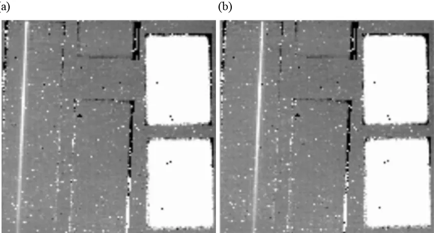
(a) (b)

Figure 2.1. (a) Nod position 1 for a Short-Low first order observation of HV 5715 (AOR#1_{: 22419456). (}_b₎

Nod position 2 for a Short-Low first order observation of HV 5715. In each image, the white color refers to positive values, the black color refers to negative values, and grey refers to values around zero. On the left side of each image, it shows the first order sub-slit projection area. The slit’s projection would be a long rectangle that is two pixels wide in the vertical direction. The wavelength changes vertically and the spatial position changes horizontally. Windows in the middle area of the image are second order projection with the “bonus” order (a 1st order segment) at top middle. The two rectangular windows shown on the right side are peak-up arrays at 16 µm and 22 µm.

(33)

[image:33.612.95.516.111.340.2]

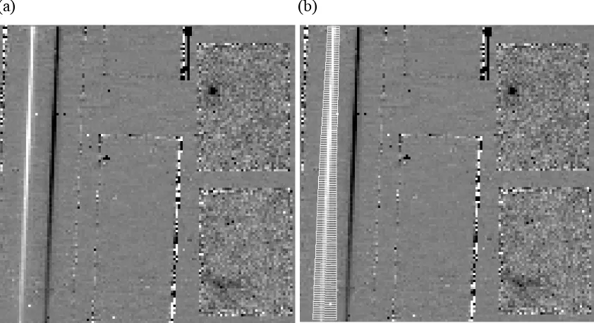
(a) (b)

Figure 2.2. (a) Nod subtracted image (nod 1 - nod 2) for a Short-Low first order observation of HV 5715.

(b) Illustration of raw signal extraction windows (white boxes) for each wavelength for the data image (a).

The third step is signal extraction. In this step, first determine the width of the signal extraction region, increasing in width proportionally according to wavelength (Eq. 2.1). Then add a pseudo-rectangle centered on the PSF’s center at each wavelength, with the width determined previously, onto the image (Kemper et al. 2010). Within the SMART, this is known as “tapered-column” window. After placing the extraction window, then simply sum the pixel signal for each wavelength element to get the signal at each wavelength. Then plot the spectrum as wavelength vs. signal strength. This step finally transfers the processed slope image into a single spectrum from 5 to 38 µm, but this is just a raw spectrum since the intensity is still in signal unit not flux unit.

(34)

spectrum from observation and a theoretical spectrum. Then we will compute a relative spectral response function (RSRF) by simply dividing the calibrator theoretical spectrum

𝐶! 𝜆 by calibrator raw spectrum 𝐶! 𝜆 . The final spectrum of a star’s 𝐹 𝜆 in Jy equals the raw spectrum of this star 𝑅 𝜆 times the RSRF:

𝐹 𝜆 = 𝑅 𝜆 ∙𝐶_𝐶! 𝜆

! 𝜆 . (2.2)

[image:34.612.90.515.425.638.2]

As long as both 𝑅 𝜆 and 𝐶_! 𝜆 are obtained by the exact same shape of truncated window, then the final spectrum will be valid, because the same track of the PSF is observed for both target and calibrator at each wavelength. A tapered extraction window is typically used. For the same reason, the unwanted effects of the PSF by the slit aperture and flat fielding are automatically removed by applying the RSRF. Figure 2.3 summarizes the entire data reduction procedures for Spitzer-IRS.

(35)

(36)

2.2 ISO Observations and Data Reduction

2.2.1 Infrared Space Observatory Telescope and SWS Instrument

ESA’s Infrared Space Observatory (ISO) was launched by an Ariane 4 rocket on Nov. 17, 1995 (Kessler et al. 1996) and operates at over wavelengths from 2.5 µm to 240 µm. Its primary mirror is 60 cm in diameter. The telescope has three-axis-stabilization systems providing pointing accuracy of a few arc seconds and is cooled to 2-8 K by a large cryostat containing 2300 liters of superfluid helium (Kessler et al. 1996). ISO has an Earth’s orbit of a period just below 24 hours. It is operated in a service-observing mode with each day’s observations being planned in detail up to 3 weeks in advance (Kessler et al. 1996).

ISO has four instruments, including an imaging photo-polarimeter ISOPHOT; a camera, ISOCAM; a short wavelength spectrometer, SWS (where our data are from); and a long wavelength spectrometer, LWS (Kessler et al. 1996). Each instrument was built separately by an international consortium of scientific institutes and industry, but all four of them were designed to form a complete and complementary package. Only one instrument is operational at a time.

(37)

working simultaneously. The SWS has three entrance apertures, each with their own beam splitters hitting both SW and LW sections, so that each aperture is used for both SW and LW sections. The transmitted beams enter the SW section, and reflected beams enter the LW sections and FPs.

SW has two detector arrays, 12 InSb detectors and 12 Si:Ga detectors, both operated at a temperature of 4 K, working on the first two bands that range from 2.38 µm to 12.0 µm (Leech et al. 2003). Each detector scans through the whole band to which it is assigned. Each grating has its own scanning devices, so both sections of SWS can be used at the same time. In order to change the wavelengths falling onto the detectors, the flat mirrors close to each grating rotate in discrete steps. There are four band segments in band 1 and three in band 2. Similarly, LW also has two detector arrays, 12 Si:As detectors working at 4 K and 12 Ge:Be detectors cooled to 2.5 K. LW is assigned to bands 3 and 4, with wavelengths ranging from 12.0 µm to 45.2 µm (Leech et al. 2003). There are three extra sub-bands added to LW as a check on the band 3 data, and they repeat the wavelength steps of the first three band segments of band 3, which has 4 band segments in total. Band 4 only has one real segment from 29 µm to 45.2 µm (Leech et al. 2003). Thus, the spectrum produced by SW and LW sections, ranging from 2.38 µm to 45.2 µm, is divided into 12 segments total (AOT bands). The FP components use mainly Si:Sb detectors that are cooled to 10 K, working at bands 5 and 6, 11.4 µm to 44.5 µm, divided into 5 FP AOT bands (Leech et al. 2003). Their spectral resolution can pass 30000, and 20000 at the lowest, whereas the spectral resolution of the first four bands reach from 1000 to 2000 as mentioned earlier (Leech et al. 2003).

2.2.2 SWS Observing Modes and Data Reduction

(38)

S01, S02, S06 and S07. But one can use a variety of AOTs and Calibration Uplink System (CUS) to do calibration observations (Leech et al. 2003). There are two main SWS observation modes: the grating-only mode where two SWS gratings work in parallel, producing medium spectral resolution, and the FP grating combination mode, where FP operates in parallel with SW grating section, producing high spectral resolution. AOT S01, S02 and S06 belong to the first observation mode, where 1 × 12 detectors are used at a time. In an operation, the grating was scanned in small steps to fully sample the target wavelength range, and a certain redundancy is provided. AOT S01 provides a quick scan of the full SWS wavelength range with 4 scan speeds from which to choose. Both S02 and S06 perform at full spectral resolution with S02 designed to measure line profiles and S06 designed for observing long wavelength regions. AOT S07 belongs to the second mode, where the spectrum is measured by varying the gap between Fabry-Pérot etalons. In this AOT, priority is given to the FP (de Graauw et al. 1996). All grating observations employed up-down scans. The grating initially scans a wavelength range in one direction and then reverses back to cover the same wavelength region in the other direction, resulting in two scans in total (Leech et al. 2003). One of the basic AOT strategies is to take dark current measurements regularly. Compared to Spitzer-IRS, there is no need to do sky subtraction by pointing to different sky. This is a direct benefit of ISO having moving parts, unlike Spitzer.

(39)

also with half reset interval, resulting in same resolving power as speed 2. Note that for all the speed modes, the recorded spectra will still have the same sampling rates across the wavelength, because the total number of samples stays the same. As a result, the integrations of these extra samples smooth the spectrum, preventing aliasing problems due to insufficient sampling. But their effective resolutions are still degraded. This means the spectrum obtained by speed mode 1 is 8 times interpolated to appear a higher spectral resolution, but its effective resolution is unchanged (Leech et al. 2003). The grating moves during a reset interval. The time line of an AOT S01 observation starts with pointing aperture 1 to target. And then it switches to aperture 2 and 3 in sequence after a single up-down scan in between to measure certain band segments. Upon completing all the up down scans, all 12 band segments will be measured. Dark current is recorded at each aperture change and at both the start and the end of each measurement. The procedure finishes with an internal photometric calibration.

In AOT S01, there are 12 detectors working for the same band, and each performs two scans (up and down) for one measurement, resulting in 24 integrations per resolution element (de Graauw et al. 1996). As we already know, there are 12 band segments in a full spectrum that SWS gives. So that is 24 × 12 = 288 spectra that need to be combined into a single coherent spectrum (Sloan et al. 2003). Before that, first we look at how the raw signals from each detector come to a segment spectrum.

(40)

wavelengths (Leech et al. 2003). This results in a table (SPD) of corrected slopes, which should be proportional to the flux density of the target. After getting SPD, the pipeline applies further corrections and calibrations, such as flat-fielding and photometric checks, to the slope data and converts slopes to fluxes (Leech et al. 2003). It results in fully calibrated fluxes as a function of wavelength. The AAR files are just like FITS files in

Spitzer-IRS, so it can also be called FITS AAR files.

Each AAR file contains the data from one observation as a series of wavelength elements. For each wavelength element, the AAR gives a series parameters other than wavelength and flux, such as uncertainty, error flags, detector number, scan number, and segment number. Sloan et al. (2003) demonstrated that there are two major problems in the process of combining spectral segments from AARs into one coherent spectrum. First, discontinuities appear between spectral segments. Second, the data in each spectral segment show significant scatter, although the scatter from a single detector in one scan direction is not prominent. This is due to the difficulty of properly aligning spectra from different detectors and scan directions. To handle these two problems, Sloan et al. (2003) developed a post-pipeline processing algorithm they called swsmake, which first combines the 24 spectra in each spectral segment into one, and then combines the 12 spectral segments into a single continuous spectrum by normalizing the segments to each other.

(41)

is under-sampled. Thus, the median is filtered so that it follows an approximate continuum, to avoid improper influence of spectral lines. As a result, the algorithm preserves the detailed spectral structure in each spectrum while removing the overlying deviations.

(42)

Figure 2.4. ISO SWS data reduction steps

G. C. Sloan et al. processed (as explained by Sloan et al. 2003) and presented a complete set of uniformly processed SWS full-scan spectra, which are the most processed form available from the ISO archive. The spectral atlas is available to the community on-line, from which we obtained our observed spectra data1.

(43)

Chapter 3

Modeling and Analysis

3.1 Problem Clarification

(44)

Figure 3.1. Possible dust and gas positions of an AGB star

As shown, the gas may exist between the dust and the stellar photosphere, or out side of the dust layer or within the dust layer or even the combination of the three. Hence, the radiation we see coming from the star travel through the following path (Figure 3.2). Our first task is to determine the final radiation intensity that reaches us from the AGB star.

(45)

3.2 Generating the Model

3.2.1 Radiative Transfer

In order to calculate the radiation intensity, we need to use the physics of radiative transfer. A change in intensity results from emission and absorption is

𝑑𝐼! = −𝛼!𝐼! +𝑗! 𝑑𝑠, (3.1)

where 𝐼_! is the original intensity, 𝛼_! is absorption coefficient, 𝑗_! is emission coefficient, and 𝑑𝑠 is the path increment. In this equation, the 𝛼_!𝐼_!𝑑𝑠 part is the absorption increment, and the 𝑗!𝑑𝑠 part is the emission increment (Rybicki & Lightman 1979). By introducing

the optical depth 𝜏_!, define 𝑑𝜏_! = 𝛼_!𝑑𝑠, and source function 𝑆_! = 𝑗_!/𝛼_!. Then Eq. 3.1 becomes

𝑑𝐼_! = −𝐼_! +𝑆_! 𝑑𝜏_!. (3.2)

The transfer function’s formal solution is

𝐼_! 𝜏_! = 𝐼_! 0 𝑒!!!₊ !!_𝑒!(!!!!!!) !

𝑆_! 𝜏′_! 𝑑𝜏′_! (3.3)

(Rybicki & Lightman 1979). When the source function is constant, the solution becomes

𝐼_! 𝜏_! = 𝑆_!+ 𝐼_! 0 −𝑆_! 𝑒!!!₍₃_.₄₎

(Rybicki & Lightman 1979), in which, 𝐼! 0 is the background intensity, and 𝑆! is the

source function of the foreground medium. Equation 3.4 shows us if 𝐼_! 0 > 𝑆_!, then

𝐼_! 0 −𝑆_! 𝑒!!!_{< 0,}_𝐼

! tends to decrease along the way, which gives us an absorption

(46)

tends to increase along the way, which then gives us an emission feature (if the optical depth profile is non-zero). This equation also shows us if 𝜏! >> 1, then 𝐼! 𝜏! →𝑆!. This

tells us if the medium is optically thick, the emergent intensity tends to be same as the source function. This also means that, for any 𝜏_!, the emergent intensity cannot pass below (for absorptions) or above (for emissions) the source function. This is a very important conclusion and a very useful criterion that will be used in our model fitting. We also see from Eq. 3.4 that in order to model the observed spectrum, we need to know the optical depth profile of the medium responsible for the spectrum, the background intensity, and the source function. Then we can use the equation 3.4 to calculate the emergent intensity, which then can be compared to the observed spectrum.

Due to local thermodynamic equilibrium (LTE; See explanation from Siegel & Howell 1981), 𝐼_! is independent of any properties related to its enclosure and only depends on the temperature at a single frequency ν (Rybicki & Lightman 1979). Basically, the second law of thermodynamics cannot be violated. So 𝐼_!(0) must be a universal function of 𝑇! and ν, which leads to Plank’s blackbody function, so we have

𝐼_!(0)= 𝐵_! 𝑇_! (3.5)

𝐵_! 𝑇 =2ℎ𝜈!

𝑐!

1

𝑒!!"! −1

. (3.6)

And according to Kirchhoff’s Law, for optically thick media, thermal radiation becomes blackbody radiation (Rybicki & Lightman 1979). Thus, 𝑆_! also equals to 𝐵_! 𝑇 ,

𝑆! =𝐵! 𝑇 . (3.7)

Then Eq. 3.4 becomes

(47)

where the background blackbody has temperature 𝑇!, and the foreground source medium

has a blackbody temperature of 𝑇. So now the final intensity becomes much easier to calculate.

3.2.2 Problem Simplification

In order to apply the radiative transfer equation 3.8 to the problem described in Section 3.1, we need to find out which physical entity each variable refers to. Since the dust shell is considered to be optically thick, 𝜏_! >> 1, and we assume LTE, then the blackbody radiation of the dust shell would be the background intensity (see earlier discussion in Section 3.2.1), which is a blackbody function, we write it as 𝐵_! 𝑇_! , where

𝑇_! is the temperature of the dust. Then the gas outside of the dust shell would be the source medium, we write its source function as 𝐵_! 𝑇_! , when we assume the gas only has one species and a single gas temperature 𝑇_!. Then the model in figure 3.2 becomes much simpler as follows:

(48)

And Eq. 3.8 becomes

𝐼_! = 𝐵_! 𝑇_! + 𝐵_! 𝑇_! −𝐵_! 𝑇_! 𝑒!!!. (3.9)

So the final intensity, observed by us, is determined by the dust temperature, gas temperature, and the optical depth of the gas layer.

Notice that we assume the gas layer only has one temperature, as we assume LTE. But we know this may not necessarily be the case. So in reality, most likely, the gas layer will have more than one temperature, (or have continuous changing temperatures) as well as more molecular species. But we opt for simplicity and looking for the major determine factors, so this simple model would still be a nice approach that we can use, especially for fitting and analysis of LMC stars. As for situations where more than one gas species, like in the galactic AGB stars, or more than one single gas temperature are needed, we can add more gas layers onto the initial model. We will use multiple gas layers associated with their own optical depth profiles instead of one single gas layer, because the optical depth profile is hard to generate when all the different type of gases are mixed together. So instead, we assume they are separated and located in a sequence as shown in figure 3.4.

(49)

Correspondingly, Eq. 3.9 finally becomes

𝐼_! = 𝐵_! 𝑇_! + 𝐵_! 𝑇_! + 𝐵_! 𝑇_! + 𝐵_! 𝑇_! −𝐵_! 𝑇_! 𝑒!!! ₋_𝐵

! 𝑇! 𝑒!!! 𝑒!!!

= 𝐵_! 𝑇_! + 𝐵_! 𝑇_! −𝐵_! 𝑇_! 𝑒!!! + 𝐵_! 𝑇_! −𝐵_! 𝑇_! 𝑒!!!!!!

+ 𝐵_! 𝑇_! −𝐵_! 𝑇_! 𝑒!!!!!!!!!, (3.10)

where 𝑇_!, 𝑇_!, 𝑇_! are gas temperatures for each gas species, and 𝜏_!, 𝜏_!, 𝜏_! are corresponding optical depth at frequency 𝜈 for that species. Notice we have a sequence in gas layers. Let us see if the result will be different if the gas layers change order. For simplicity, consider only two gas layers. Eq. 3.9 will be

𝐼_! = 𝐵_! 𝑇_! + 𝐵_! 𝑇_! + 𝐵_! 𝑇_! −𝐵_! 𝑇_! 𝑒!!! −𝐵_!(𝑇_!) 𝑒!!!

= 𝐵_! 𝑇_! + 𝐵_! 𝑇_! −𝐵_! 𝑇_! 𝑒!!! + 𝐵_! 𝑇_! −𝐵_! 𝑇_! 𝑒!!!!!!. (3.11)

When gas1 and gas2 layer switch place, then it becomes

𝐼_!′= 𝐵_! 𝑇_! + 𝐵_! 𝑇_! + 𝐵_! 𝑇_! −𝐵_! 𝑇_! 𝑒!!!₋_𝐵

!(𝑇!) 𝑒!!!

= 𝐵_! 𝑇_! + 𝐵_! 𝑇_! −𝐵_! 𝑇_! 𝑒!!! + 𝐵_! 𝑇_! −𝐵_! 𝑇_! 𝑒!!!!!!. (3.12)

The results show that they are not equal to each other, even if we let τ1 = τ2 (same species), meaning the sequence of the gas layer in this model is not interchangeable. But if consider 𝑇_! = 𝑇_! = 𝑇,

𝐼_! =𝐼_!! ₌ _𝐵

! 𝑇 + 𝐵! 𝑇! −𝐵! 𝑇 𝑒!!!!!!. (3.13)

(50)

since changing the order of different temperature media will change the absorption and emission quantity, thus change the final intensity. This also confirms our concern of the weakness of our model if in reality different gases are mixed together. But the fact is that, when multiple species are mixed together, the optical depth will no longer be calculable, as we are assuming the medium to be homogeneous to calculate the optical depth profile (see Section 3.3). So the multiple-layer model is rather the best we can achieve (while not too complicated), considering all the assumptions and equations we have.

3.2.3 Background Continuum

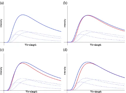
We assumed the background continuum is a single blackbody function, due to LTE. In reality, the dust shell will have different temperatures in different regions, as the shell is spatially very large. So in that case, the real dust background continuum is more likely to be a summation of blackbody functions consisting of a series of different temperatures or continuously changing temperatures within a certain range. Figure 3.5a demonstrates background continuum arising from three blackbody functions at different temperatures. As we can see, when we try to fit this continuum (in blue) with a single blackbody function (in red), it cannot be perfectly fitted (Fig. 3.5 b). If we try to fit only the shorter wavelength region of continuum, though the longer wavelength part of the continuum will not be modeled well, the shorter wavelength part can be fitted fairly well (Fig. 3.5c). Similarly, if we fit only to the longer wavelength continuum, we can fit it fairly well, but the shorter wavelength continuum will not be fit well (Fig. 3.5d).

(51)

(a) (b)

Wavelength Wavelength (c) (d)

[image:51.612.90.517.105.421.2]

Wavelength Wavelength

Figure 3.5. (a) This sample background continuum (solid blue line) consists three blackbody functions at

different temperatures (dashed blue line). (b) Fitting continuum (blue) with a single blackbody function (red). (c) Fitting the longer wavelength region with a single blackbody function. (d) Fitting the shorter wavelength region with a single blackbody function.

(52)

3.3 Optical Depth Profile

Now we determine optical depth, 𝜏!. Optical depth describes how much absorption

occurs when light travels through an absorbing medium. If the optical depth is large, when 𝜏! >> 1, we say the region is optically thick, light is readily absorbed. On the other

hand, If the optical depth is small, when 𝜏_! << 1, the region is optically thin, and light passes through easily.

According to Cami et al. (2010), the optical depth at frequency ν due to a transition i for a homogeneous medium is determined by

𝜏_!! ₌_𝑁_∙_𝑆

!!!∙𝜙!, (3.14) where, 𝑁 is column density, which is the number of scatterers lying within a column of a certain area along the whole distance the light travels through that medium, and it has units of cm-2. 𝑆! ! is the line strength at the center frequency 𝜈! of transition i, and 𝛷! is

line profile function. We use a Gaussian profile as described in Cami et al. (2010) for 𝛷!:

𝛷_! = 1

Δ𝜈_!𝑒!(!!!!) !_/_(!_!

!)!. (3.15)

We know that many physical effects determine the line shape. Here we assume the Doppler effect is the main reason of line broadening, and this will be explained later in Section 3.4. The Doppler width 𝛥𝜈_! is a combination of both thermal motions and micro-turbulent motions,

Δ𝜈_! =𝜈!

𝑐

2𝑘𝑇

𝑚_! +𝜐!"#$! !

!

(53)

(Cami et al. 2010), where 𝑚! is the mass of the molecules, 𝜈! is the central frequency of

the line, 𝑇is the temperature of the gas, and 𝜐_!"#$ _{is the microturbulenct velocity. Eq.} 3.16 is later replaced by Eq. 3.21 and 3.22 (see Section 3.5). Thus, with parameter 𝑁, 𝑇

and 𝜐! (𝜐!"#$ is included in 𝜐! in our paper, see Section 3.5), we can generate optical

depth profiles for a certain molecule. We will discuss all the values we adjusted for these parameters later in Section 3.11 and in Chapter 4. Basically our goal is to determine the values of 𝑁, 𝑇 and 𝜐_! _{, by comparing the calculated and observed line profiles, and then} try to interpret the possible corresponding physical meaning.

(54)

3.4 Line Broadening Effect

Now let us take a look at the causes of line broadening effect, and how it affects the line profile function. Basically, the causes of line broadening effect can be categorized into two categories: microscopic and macroscopic.

3.4.1 Microscopic Line Broadening

Microscopic broadening mechanisms occur on length scales smaller than the photon mean free path. Typically such processes operate on an atomic scale. These microscopic processes change the optical depth profile of the absorber by changing its profile function, thus further affecting the absorption features of the absorber. Primary types of microscopic broadening processes responsible for absorption feature include thermal broadening, natural broadening, and microturbulent broadening.

Thermal broadening is caused by Doppler effect from random thermal motion. We know that the thermal velocity (most probable speed of thermal movements) is equal to

2𝐾𝑇/𝑚. For AGB stars we are interested in, that speed is around 1 km/s for gases outside of the dust shell. The corresponding width of spectral line due to thermal broadening is on the scale of 10-1 nm. The thermal motions of molecules have Maxwell-Boltzmann velocity distribution, which when projected onto a single axis will result in a Gaussian distribution of the spectroscopic radial velocity. This Gaussian function will be the profile function for calculating optical depth profile.

(55)

on the order of 10-8_{s (comes from the reciprocal of the Einstein coefficient of} spontaneous emission), the line width of natural broadening can be estimated using uncertainty principle relationship between time and energy, and is on the scale of 10-3 nm for gases outside of the carbon stars. So the natural broadening can be neglected when compared to the thermal broadening.

The “microturbulent” broadening process is not well defined physically. It arises from mechanisms causing line broadening other than thermal motions. This typically includes internal small-scale motions within an interstellar cloud. Without a firm physical model for these additional sources of velocity dispersion, it is customary (and convenient) to adopt a Maxwell-Boltzmann velocity distribution the same as for thermal motions, for microturbulent motions1, which will also have a Gaussian radial (line-of-sight) velocity distribution. Hence, We assume a Gaussian profile for both the microturbulence and the thermal motions in the line profile function. The Doppler velocity of microturbulent is reported to be around 2.5 km/s in the stellar photosphere (Aringer et al. 1997).

3.4.2 Macroscopic Line Broadening

Macroscopic broadening processes operate on length scales greater than the photon mean free path. Examples are Doppler broadening caused by stellar rotation and pulsation (expansion), as well as stellar outflow. These types of movements are in the macroscopic scale across the whole star shell, and bring Doppler effect due to blue shift and red shift at different regions of the star. Stellar outflow (expansion) velocities of carbon-rich AGB stars are reported to range from 3 to 40 km/s with most of them at around the mean value 17 km/s (Marigo et al. 2008).

1_{See p. 65 in the lecture notes (accessible through http://zuserver2.star.ucl.ac.uk/~idh/PHAS2112) of the}

(56)

(57)

3.5 Doppler Broadening Velocity

As discussed above, the line broadening processes that will affect our results are three types of Doppler broadening: the thermal, the microturbulent and the macroscopic ones. The first two of them can already be quantified and represented by Doppler width and Gaussian profiles. Let us take a look at the third one.

As described above, regarding macroscopic Doppler broadening, the final flux density we obtained is the result of the original line convolved with a Doppler shift profile of macroscopic broadening processes. We can assign 𝐷(𝜈) to represent this Doppler profile. So the new intensity in Eq. 3.8 would become

𝐼_!! ₌ _𝐵

! 𝑇 + 𝐵! 𝑇! −𝐵! 𝑇 𝑒!!! ∗𝐷 𝜈 . (3.17)

If we use optically thin approximation for gas layers to get an estimate of the Doppler effect, we will have

𝑒!!! ≈ 1−𝜏_!, (3.18)

then Eq. 3.17 becomes

𝐼_!! ₌_𝐵

! 𝑇! ∗𝐷 𝜈 + 𝐵! 𝑇! −𝐵! 𝑇 𝜏!∗𝐷 𝜈 . (3.19)

A blackbody function convolves with a Doppler profile is still the blackbody function. So we further have

𝐼_!! ₌ _𝐵

! 𝑇! + 𝐵! 𝑇! −𝐵! 𝑇 (𝜏! ∗𝐷 𝜈 ). (3.20)

(58)

resolution and cannot resolve fine lines, it should not matter what shape the exact Doppler profile looks like, as long as it provides us the equivalent broadening width. That means if we use a new Doppler width 𝛥𝜈! to replace Eq. 3.16, then we will have a new

optical depth profile that accounts for all the Doppler broadening effects. So we have

Δ𝜈_! = 𝜈!

𝑐 𝜐! (3.21)

to replace Eq. 3.16. We call 𝜐_! the Doppler broadening velocity, and it is a combination of the thermal velocity 𝜐!!, the microturbulent velocity 𝜐!"#$, and an equivalent star

expansion velocity 𝜐_!"#! _{- in our case, macroscopic velocities are mostly caused by the} expansion rate of the circumstellar shell around the AGB stars:

𝜐_! = 𝜐_! _!!₊_𝜐

!"#$ !+𝜐!"#! !

!/!

. (3.22)

We need to determine what is the relationship between 𝜐_!"#! _{and the real expansion} velocity 𝜐_!"# _{in order to have the correct equivalent broadening width. Considering the} expansion speed is very small compared to the speed of light, 𝜐_!"# _<<_c_{, the low speed} approximation for relativistic Doppler shift of light wave gives us

Δ𝜈 = 𝜈_!

𝑐 𝜐!"# . (3.23)

The Δ𝜈 is the estimate of the broadening width caused by the shell’s expansion, because the spectroscopic radial velocity (which actually causes the broadening effect) for the different parts of the circumstellar shell will range from 0 (since the - 𝜐_!"# _{side is blocked} by the star itself thus cannot be observed by us) to 𝜐!"# . And we know the broadening

width (namely full width at half maximum, FWHM) caused by 𝜐_! _!_or_𝜐

!"#$ is 1.6651

1_{For the derivation of 1.665, see p. 64 in the lecture notes (accessible through}

(59)

times larger than its Doppler width Δ𝜈! appeared in Eq. 3.16 and 3.21. So similarly, for 𝜐_!"#! _{, we have:}

Δ𝜈= 1.665 Δ𝜈_!(_!"#₎ = 1.665𝜈!

𝑐 𝜐!"#! . (3.24)

where Δ𝜈!(!"#) is the Doppler width caused by star expansion. Combining Eq. 3.23 with 3.24, we can easily see

𝜐_!"# ₌₁_.₆₆₅_𝜐

!"#! . (3.25)

Therefore, considering the expansion velocity range (3 to 40 km/s) and its mean value 17 km/s, plus microturbulent velocity of 2.5 km/s and the thermal velocity around 1 km/s, the estimated overall Doppler velocity 𝜐! would range from 3 km/s to 24 km/s with

(60)

3.6 Line Strength

Line strength 𝑆_! _!_{, which appears in Eq. 3.14, describes the intensity of a spectral}

line at a given frequency. It is related to the net rate of absorption (or emission) at that frequency. Cami et al. (2010) gives the line strength 𝑆! ! at temperature T for a transition

at frequency 𝜈_!_{from a lower level 1 to an upper level 2 as}

𝑆!! 𝑇 =

ℎ𝜈_!

4𝜋 𝑔!𝐵!"

𝑒!!"!!

𝑃 𝑇 1−𝑒!!

!!

!" ₍₃_.₂₆₎

𝑃 𝑇 = 𝑔_!𝑒!!!/!" !

, (3.27)

where ℎ𝜈_! = 𝐸_! - 𝐸_!, 𝑔_! 𝑖𝑠 statistical weight of the lower level, 𝐵_!" is the Einstein coefficient of stimulated absorption. 𝑃 𝑇 is the partition sum, running over all molecular levels, and 𝑔_! is the number of quantum states that have the same energy level. The partition sum plays the role of a normalizing constant. It encodes how the probabilities are partitioned among the different microstates, based on their individual energies. It contains all the transitions of different energy levels or microstates, such as electronic, vibrational, and rotational contributions. So the exact calculations of these partition functions at different temperatures are evaluated using quantum mechanical methods (Sauval & Tatum 1984).

If we know the line strength at