Re-creation of site-specific multi-directional waves with non-collinear current

Re-creation of site-speci

fi

c multi-directional waves with

non-collinear current

S. Draycott

, D.R. Noble

, T. Davey

, T. Bruce

, D.M. Ingram

, L. Johanning

,

H.C.M. Smith

, A. Day

, P. Kaklis

a_{FloWave Ocean Energy Research Facility, Max Born Crescent, King's Buildings, Edinburgh, EH9 3BF, UK} b_{Institute for Energy Systems, School of Engineering, The University of Edinburgh, Edinburgh, EH9 3JL, UK} c_{College of Engineering, Mathematics and Physical Sciences, University of Exeter, Penryn Campus, TR10 9FE, UK} d_{Naval Architecture, Ocean and Marine Engineering, University of Strathclyde, Glasgow, G4 0LZ, UK}

A R T I C L E I N F O

Keywords:

Wave-current interactions Site-specific wave conditions Directional wave spectra Directional spectrum measurement Tank testing

A B S T R A C T

Site-specific wave data can be used to improve the realism of tank test conditions and resulting outputs. If this data is recorded in the presence of a current, then the combined conditions must be re-created to ensure wave power, wavelength and steepness are correctly represented in a tank. In this paper we explore the impacts of currents on the wavefield and demonstrate a simple, effective methodology for re-creating combined wave-current scenarios. Regular waves, a parametric unidirectional spectrum, and a complex site-specific directional sea state were re-created with current velocities representing 0.25, 0.5, and 1.0 m/s full scale. Waves were generated at a number of angles relative to the current, providing observations of both collinear and non-collinear wave-current interactions. Wave amplitudes transformed by the current were measured and corrected linearly, ensuring desired frequency and wavenumber spectra in the presence of current were obtained. This empirical method proved effective after a single iteration. Frequency spectra were within 3% of desired and wave heights normally within 1%. The generation-measurement-correction procedure presented enables effective re-creation of complex wave-current scenarios. This capability will increase the realism of tank testing, and help de-risk devices prior to deployment at sea.

1. Introduction

Tank testing of physical scale models is an essential element in the development of marine renewable technologies and techniques. Under-taking this testing in laboratories provides a controlled, repeatable, and low-risk environment where technological concepts and operational techniques may be developed (Ingram et al., 2011). Afive-stage struc-tured development plan for wave energy systems was outlined byHolmes and Nielsen (2010), which can be related to the widely used Technology Readiness Level (TRL) concept, developed initially by NASA (Mankins, 1995). Using scaled sea conditions based on open sea measurements at wave energy sites when tank testing renewable energy devices, particu-larly at mid and later stage TRL levels, can improve understanding of device performance prior to deployment at sea.

The aim of this work is to explore the impacts of currents on the wave

field, and to demonstrate an effective approach to include currents in

scale model testing thus representing the combined conditions appro-priately. A site-specific directional sea state is used to illustrate this methodology, derived from the Billia Croo wave test site at the European Marine Energy Centre (EMEC). Experiments were carried out in the cir-cular wave basin of the FloWave Ocean Energy Research Facility, enabling both waves and current to be generated in all directions.

Currents change the physical form of waves, as discussed byPeregrine (1976)and others. Although the wave period remains constant, waves become steeper when they encounter an opposing current; a combination of both the wave height increasing and wavelength decreasing. Wave breaking will occur as the steepness approaches a critical limit, and faster currents prevent upstream wave propagation completely, i.e. wave blocking. With a following current the converse occurs and waves become less steep. For waves at an angle to the current, there is also refraction of the wave direction to consider.

Several experimental studies have been published on the influence of

* Corresponding author. ** Corresponding author.

E-mail addresses:[email protected](S. Draycott),[email protected](D.R. Noble).

Contents lists available atScienceDirect

Ocean Engineering

j ourna l homepa ge:www.el se vier.com/locat e/oce aneng

https://doi.org/10.1016/j.oceaneng.2017.10.047

Received 8 December 2016; Received in revised form 27 September 2017; Accepted 22 October 2017 Available online 28 October 2017

currents on waves. Early studies includingThomas (1981); Kemp and Simons (1982, 1983) used hydraulic flumes to investigate collinear wave-current interaction for regular waves. The main focus was the

in-fluence of waves and bed roughness on the current profile, although modification of the waves by the current was also included. This exper-imental work on regular waves was extended to consider uni-directional spectra with collinear currents byHedges et al. (1985)andChakrabarti and Johnson (1995). Adding more complexity, Nwogu (1993) and

Guedes Soares et al. (2000) looked at the influence of currents on directional spectra. Both studies were carried out in wave basins with a single bank of wavemakers with nozzles in front to generate current, so considered spectra with a predominantly following current. Mean wave directions of 0∘;15∘;30∘, and 45∘relative to the current were tested by

Nwogu (1993), although any modification of the frequency spectra were not reported. As far as the authors are aware, the research presented below is the first comprehensive study of oblique wave-current interaction.

Measured site wave data may be used to produce scaled sea states that capture spectral complexity and directional features not effectively rep-resented by standard parametric spectra and spreading functions (as discussed inDraycott et al. (2015)). This site data, typically gathered by a wave buoy, may have been measured in the presence of current. This current is not typically reproduced in the test tank and therefore wave power and steepness of the sea states will be misrepresented. This has potentially large implications on the assumed resource and on the val-idity of observed device response, as discussed in Section2.

The rest of the paper is organised into four sections. In Section2we explore the impact of a current on the wavefield, including implications for power and steepness if this current is omitted during testing. The experimental methodology is given in Section3, with results in Section4. Some discussion of thesefindings is then presented in Section5.

2. The effect of current on the wavefield

Currents transform the wavefield, including wave height and length, as mentioned in Section1. This alters the form of the frequency and wavenumber spectra, along with the power available. The impact of tides on wave power resource has been investigated using a numerical model byHashemi et al. (2014). This work showed the impact of tides on wave power resource could exceed 10% at sites with currents of around 1.5 m/s. Other papers such asSaruwatari et al. (2013)suggest this effect may be as large as 60% in 3 m/s currents, however current-induced wavelength and group velocity changes appear to have been ignored. This leads to an over-estimation as described in Section2.3, analogous to the described wave buoy scenario.

Wave buoys, including the Datawell Waverider©buoys deployed by EMEC, typically measure heave, pitch, and roll. The resulting frequency spectra are calculated from the heave motions (Earle, 1996), whilst the directionality is inferred through cross-correlation of the three signals. If a current is present at the site, the sea surface elevations and hence calculated frequency spectrum will therefore be altered, but without knowing the corresponding change in wavelength.

If it is assumed there was no current, wavenumber spectra calculated for the recorded frequency spectra will be incorrect, as will steepness and power. This has potentially large implications for the assumed resource available, along with the form of the waves, as explored below. Addi-tionally, if a spectrum is replicated in a test environment without current, this would fail to capture the true nature of the site conditions.

2.1. Calculation of available power and steepness

For waves in the absence of current the wavenumber for each fre-quency can be obtained from the dispersion relation Eq.(1), with cor-responding wavenumber spectrum SðkÞ and group velocities Cg

calculated from Eq.(2)and the measured frequency spectrumSðfÞ.

ω¼pffiffiffiffiffiffiffiffiffiffiffiffiffiffiffiffiffiffiffiffiffigktanhkh (1)

SðkÞ ¼SðfÞCgðfÞ

2π ; CgðfÞ ¼ 1 2

ω

k

1þ 2kh sinh2kh

(2)

whereωis the angular frequency,kthe wavenumber, andhwater depth. The total power in a wave spectrumPis calculated from Eq.(3), inte-grating component wave power.

P¼∫pðfÞδf where pðfÞ ¼ρgSðfÞCgðfÞ (3)

Significant steepnessSpis calculated from the wavelength associated

with the peak of the wavenumber spectrumLpand Eq.(4). This version of

peak wavelength has been used, rather than the wavelength associated with the peak frequency, for two reasons. Firstly, the wavelength asso-ciated with the peak of the wavenumber spectrum does not always equal that obtained fromfp, as discussed inPlant (2009). The peak energy lies

at the wavelength associated with the wavenumber peak, so using this value provides a more representativefigure for the true steepness of a sea state. Secondly, this definition allows for a consistent comparison of steepness between cases with and without current.Hm0is the significant

wave height.

S_p¼Hm0 Lp

(4)

2.2. Transformation of wave spectra in the presence of current

In the presence of current, wavelength is no longer related to fre-quency through the standard dispersion relation, Eq.(1). A modified relation, Eq. (5), is used instead (Jonsson, 1990). In the following equations,α is the angle between wave and current propagation di-rections, and subscripts 1 and 0 refer to regions with and without current respectively. Importantly, the wavenumber in the presence of a current

k1will differ fromk0.

ωk1Ucosα¼pffiffiffiffiffiffiffiffiffiffiffiffiffiffiffiffiffiffiffiffiffiffiffiffiffigk1tanhk1h (5)

Using a linear assumption, the amplitudes of each frequency componentAðfÞare given by:

AðfÞ ¼pffiffiffiffiffiffiffiffiffiffiffiffiffiffiffiffiffi2SðfÞΔf (6)

The current modified component wave amplitudes can be calculated assuming conservation of a quantity termed ‘wave action’ (Jonsson, 1990) defined as:

∂

∂x

ECgrþUcosα

ωr

¼0 (7)

whereEis the wave energy andxthe direction of wave propagation. The subscriptrdenotes variables relative to the current, i.e. assuming a frame of reference moving at the same velocity as the current. The relative angular velocitiesωrand group velocitiesCgrcan be expressed as:

ωr¼pffiffiffiffiffiffiffiffiffiffiffiffiffiffiffiffiffiffiffiffiffiffiffiffiffigk₁tanhk₁h (8)

Cgr¼ 1 2

ωr

k₁

1þ 2k1h sinh2k₁h

(9)

Equating wave action between regions with a steady currentUand with no current, Eq.(7)can be rearranged to relate the wave heights (Smith, 1997), giving component amplitudes as:

A₁¼A₀

ffiffiffiffiffiffiffiffiffiffiffiffiffiffiffiffiffiffiffiffiffiffiffiffiffiffiffiffiffiffiffiffiffiffiffiffiffiffiffiffiffiffiffiffiffiffiffiffiffiffiffiffiffiffiffiffiffiffiffiffiffiffiffiffiffiffiffiffiffiffiffiffiffiffiffiffiffiffiffiffi

Cg;0

Cgr;1þUcosα

1 1þUcosαCgr;1

s

The transformed frequency spectrum can be reconstructed using Eq.

(6), takingA1ðfÞto getS1ðfÞ. This results in the same transformation as that formulated inChakrabarti and Johnson (1995). The wavenumber spectra, power available, and wave steepness in the presence of a current can be calculated via Eqs.(2)–(4), using the relevant terms with current as appropriate.

2.3. Power and steepness assumed if wavelength and group velocity change omitted

Calculating power and steepness for waves in the presence of a cur-rent using the method in Section2.1will give incorrect results if the wavenumber transformation described in Section 2.2 is not also included. This situation could arise when using measurements from a wave buoy where there is no knowledge of the current, and thus the wavelength change. The measured transformed spectrum S1ðfÞ has

associated wavenumbers k1ðfÞ. With the assumption of no current,

wavenumbersk0ðfÞare calculated using Eq.(1), rather than using Eq.(5)

to getk1ðfÞ. This assumption leads to incorrect calculation of group

ve-locities and wavenumber spectra, hence the power and steepness will also be incorrect.

To demonstrate the effect of current on both the transformed and assumed spectra, a Pierson Moskowitz (PM) spectrum withHm0of 5 m

andTpof 8 s is used to show the effect over a wide range of frequencies.

This has been analysed with both opposing and following current ve-locities of 0.25, 0.5 and 1.0 m/s. The significant wave height is found to increase 27.6% with 1 m/s opposing current, and decrease 17.2% for 1 m/s following current.

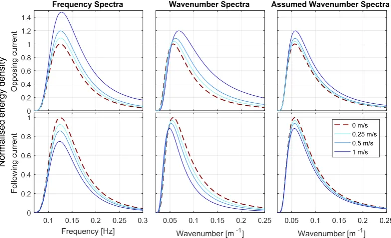
The transformation of frequency and wavenumber spectra are shown inFig. 1, along with the wavenumber spectrum that would be assumed without the knowledge of the current present. In opposingflow, waves increase in steepness and thus spectral magnitude increases, with asso-ciated reduction in wavelength shown as a shift to higher wavenumbers. The opposite is true of the following current conditions.

For the assumed case with no current there is no shift in wavenumber, and hence the steepness change will be under-estimated. In addition, the group velocity is unaltered which causes an over-estimation of the change in power. This is shown in Fig. 2, where the maximum

discrepancy is the 1 m/s opposing case, under-estimating steepness by 18.6% and over-estimating power by 26.9%. This demonstrates the importance of measuring currents at a site in order to obtain a realistic resource assessment and site characterisation.

When tank testing with realistic site conditions the associated current should be included, so that conditions mimic the site, and results inferred from the testing are representative. The correct wavenumber for each frequency component cannot be attained without the current, but are implicitly correct if the current and scaled depth are accurately repro-duced. It is important the frequency spectrum is correct in order to obtain the desired wavenumber spectra, power and steepness. At FloWave this requires a correction procedure as a result of the current transformation, so input amplitudes must be altered. This process is detailed in Section

3.4.3, and demonstrated for a range of combined wave-current condi-tions in Section4.

Fig. 1.Change in example PM spectrum (Hm0¼5 m,Tp¼8 s) in the presence of opposing and following currents. Panels show the real frequency and wavenumber spectra, along with the

wavenumber spectra assumed without knowledge of the change in wavelength resulting from the interaction with current.

3. Experimental method

3.1. The FloWave Ocean Energy Research Facility

The experimental measurements presented here were made at the FloWave Ocean Energy Research Facility, located at the University of Edinburgh. The facility is comprised of a circular 25 m diameter com-bined wave and current test basin, encircled by 168 active-absorbing force-feedback wavemakers. The water depth in the test area is 2.0 m. A re-circulatingflow system is created using 28 impeller units mounted in the plenum chamber beneath thefloor (Robinson et al., 2015). These enable a predominantly straightflow to be achieved in any direction across the central test area (Noble et al., 2015). These unique design features remove any inherent limitation on both wave and current di-rection, enabling the re-creation of complex directional sea states in combination with current.

The modification of waves by a current is of particular relevance at the FloWave facility, where the waves are generated in a region of still water around the circumference of the tank, and then interact with the current which is injected through thefloor (Robinson et al., 2015). In order to produce the desired wave height in the central test area of the tank with the presence of a current, a correction factor must be applied to the wave generated in still water, as discussed in Section3.4.3.

3.2. Site characterisation and sea state choice

The European Marine Energy Centre (EMEC) is an open water test facility for wave and tidal energy devices, with both full scale and nursery sites, based in Orkney, UK. Over the last 12 years EMEC has gained vast experience in both device installation and resource measurement at these sites.

Directional wave data from the full-scale grid connected wave test site at Billia Croo have been made available, albeit without corresponding data on currents. This EMEC dataset contains multiple years of half hourly directional sea states from January 2010 to January 2014. Rather than choosing an individual spectrum for this case study, outputs from

Draycott et al. (2014, 2015)have been used. The aim of this previous work was to produce a small subset of statistically representative spectra from the same dataset, whilst retaining the sea state complexity and directionality. The use of clustering algorithms was of particular interest as they enable the consideration of the whole spectral form in the clas-sification. In Draycott et al. (2015), 40 representative spectra were created from two years of data (January 2010 to January 2012, around 35 000 sea states) using a variety of methods. A method was chosen, which maximised intra-group similarity and inter-group distinctness, utilising a combined binning-clustering approach.

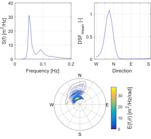
One of the resulting sea states was chosen as an example for repro-duction, representing approximately 0.14% of the dataset. This was chosen as it represents an interesting case of a: multi-modal sea state with reasonable directional spreading. The sea state has a significant wave heightHm0of 3.53 m, a peak periodTpof 20 s, and mean powerPof

87.6 kW/m wave crest. The frequency and directional spectra, along with the weighted Directional Spreading Function (DSF) are shown inFig. 3. The water depth at the wave buoy location is 52 m, relating to inter-mediate water depth for the majority of wave components present.

With no tidal records available for the site, the Atlas of UK Marine Renewable Energy (ABP MER, 2012) has been used to obtain the peak tidal velocity at the Billia Croo site, which is expected to be between 0.25 and 0.5 m/s (0.5–1.0 knots).

3.3. Test plan: wave-current scenarios

The wave current correction procedure was applied for wave condi-tions of increasing complexity. Tests were conducted with regular waves, a long-crested parametric JONSWAP spectrum, and the non-parametric directional sea state derived from the EMEC data. To facilitate

comparison, the height and period of the parametric waves were chosen to roughly match the peak of the recorded sea state (seeTable 1). Test lengths were specified as a power of 2 s to facilitate frequency domain analysis, with longer tests used to capture the detail of the direc-tional spectra.

The three different sea states (regular, parametric, and non-parametric) were tested at various relative angles to the current di-rection with three current velocities. The chosen sea states must be scaled before re-creation in the tank. Froude scaling was used to ensure the correct ratio between inertial and gravitational forces, which are dominant in free surface waves. When choosing a scale one must consider the ratio of tank to site depth along with the wave generation limits of the tank. The FloWave facility has a test water depth of 2 m and is optimised for wave generation at around 2 s period, which corre-sponds to scales around 1:20 to 1:40 for wave climates typically of in-terest to renewable energy. For waves in intermediate depth water, spectra need to be scaled by the depth ratio between tank and site. If this is not done, although the energy distribution across frequency and direction will be correct, the resulting wavenumber spectra will not. This results in a frequency dependent wavelength discrepancy. As there are no wave generation limits at the desired scale, the depth ratio of 1:26 can be used without issue. As well as scaling the wave spectra, the tidal current must also be scaled using the same relationship. At 1:26 (Froude) scale the site estimates correspond to between 0.05 and 0.1 m/ s in the tank. An additional velocity of 0.2 m/s was also used to demonstrate the method effectiveness in faster currents, where the wave-current interaction is greater.

Previous published work on wave-current interactions has largely focussed on collinear cases; waves either propagating in the same di-rection as the current, or directly opposing it. The capability of FloWave permits the testing of non-collinear cases, with the waves at an arbitrary angle to the current direction. Waves were generated at relative angles to the current of 0 (following)π=4,π=2 (perpendicular), 3π=4 andπ(opposing). For the regular wave tests, an additional four intermediate angles were also measured. A range of angles were tested to demonstrate the applicability of the method, however, when considering a real site these would be chosen based on the wave fetch and tide directions.

Fig. 3.Representative complex sea state from Billia Croo. Subplots show the spectral density SðfÞ, weighted mean directional spreading function DSFmean, and directional

3.4. Test method

The sea states defined inTable 1were initially validated in the tank without the presence of a current, confirming that they have been correctly generated prior to observing and analysing the transformation with current.

Current velocities were set based on a depth averaged calibration from measurements taken in the centre of the tank. It is noted that there is some spatial variation with reduced velocity towards the outside of the basin due to the method of producing current in the circular tank (Noble et al., 2015). The potential implications of this are explored in Section

5.2. Velocity measurement using an Acoustic Doppler Velocimeter (ADV) ensured that the current had reached an equilibrium prior to wave generation.

3.4.1. Directional sea state generation

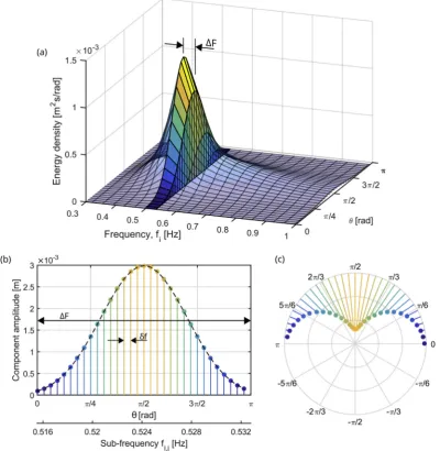
Deterministic waves are generated at FloWave, providing a very high degree of repeatability (Ingram et al., 2014). To generate a directional spectrum using this deterministic approach the single-summation, rather than double-summation method is used, depicted in Fig. 4. This avoids a phenomenon called phase-locking (Miles and Funke, 1989), whereby waves with the same frequency

but different directions interact and cause spatial patterns, resulting in a non-ergodic wavefield. To avoid this, the initial frequency increments

ΔF can be split up further to create sub-frequency increments δF¼ ΔF=Nθas shown inPascal (2012). These new frequency increments, still within the original frequency bins, now have a unique wave propaga-tion direcpropaga-tion associated with each of them.

The single-summation approach used also aids in both the sea state measurement and the implementation of correction factors. When ana-lysing results in the frequency domain each measured component amplitude can be identified and operated on individually, but only if the Fast Fourier Transform (FFT) bins match the generation frequencies. This is key to the correction method, and means that the appropriate correc-tion factors can be identified and applied, for each of the sub-frequencies. Essentially this allows different correction factors to be applied for the various relative current angles, which is vital for correcting directional seas with current.

The directional sea states presented here have a repeat timeTof 2048 s, defining the sub-frequency incrementsδf to be 1/2048 Hz. In order to achieved the desired frequency increments, the scaled spectrum was interpolated to create 64 frequency bins between 0 and 1 Hz, and 32 directional bins from 0π, covering the region with significant energy content in the directional spectrum (Nf¼64;Nθ¼32). Re-defining the

directional spectrum for use in the single-summation method gives the required frequency increments of:

δf ¼ΔF N_θ ¼

1

NfNθ

¼1

T¼

1

2048½Hz (11)

3.4.2. Directional wave measurement

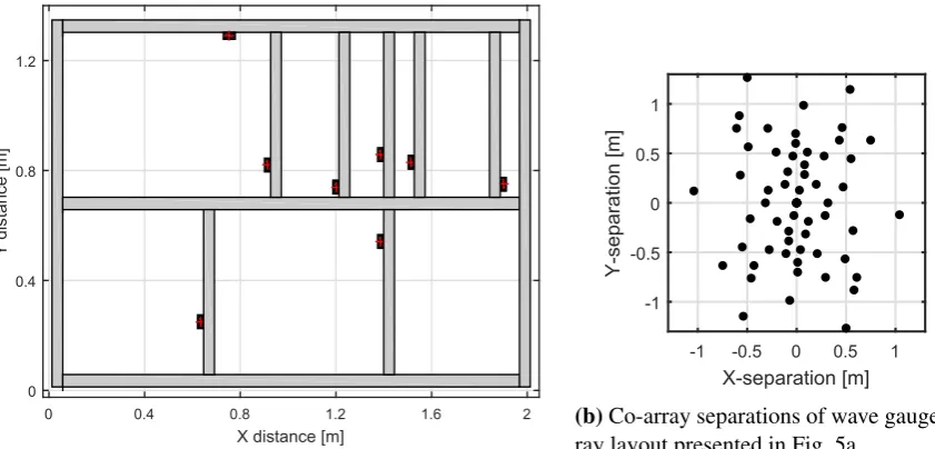
Surface elevations are measured at FloWave using multiplexed two-wire resistance type wave gauges, providing point measurements at a sample frequency of 128 Hz. In order to calculate component wave di-rections and infer directional spectra, these wave gauges are deployed in a carefully designed array (Draycott et al., 2016), shown inFig. 5a. The array has been chosen to encompass desirable spacings for the analysis, and is based on optimising the co-array uniformity over the angle and magnitude range of interest. This co-array is shown inFig. 5b, providing favourable separations for the calculation of directional spectra.

A Phase-Time-Path-Difference (PTPD) approach (Fernandes et al., 2000; Esteva, 1976) has been used to calculate component angles and directional spectra. This method uses the measured phase differences, and known separations between gauges, to infer the wave direction at each frequency, and provides a single wave angle per frequency through triangulation.Draycott et al. (2016)has shown this method to be a highly effective approach for measuring directional spectra when combined with single-summation wave generation. For measuring directional wave characteristics in currents, this approach has also found to be much more effective as discussed in Section5.3, and as such has been applied here. In

addition to reducing directional spectrum reconstruction error, the PTPD outputs provide individual component wave angles, opening up the possibility of effectively assessing wave refraction in current.

3.4.3. Correction procedure

To produce waves of a specified height in combination with a current, an amplitude based correction factor needs to be applied to the wave-maker input. For a directional spectrum, it is necessary to determine this factor for every frequency and direction component. As a result of using a single summation method, see Section3.4.1, the amplitude of each wave component with unique frequency and direction Aiðfi;θiÞcan be

cor-rected. These correction factor are assumed linear, taken as the inverse of the change in component amplitude as a result of the interaction with the currentfield discussed in Section2.2, and are calculated empirically. The input wave spectrum is generated in the tank with current, measured, and the resulting component amplitudes compared with those desired, Eq.(12). The correction based on observed discrepancy between the desired and measured directional spectra was multiplicatively applied to the input spectrum, and the process repeated as necessary in an iterative manner until the measured spectrum was acceptably correct, defined in this case as a mean spectral errorε<5%, Eq.(13).

CFempirðfi;θiÞ ¼

Adesired i Ameasured i (12) ε¼

PNf

i¼1jSmeasuredðfiÞ SdesiredðfiÞj PNf

i¼1SdesiredðfiÞ

(13)

4. Results

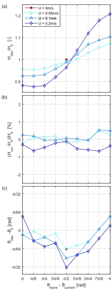
4.1. Regular waves

The observed change in wave height as a function of relative angle and current velocity can be seen inFig. 6a. As expected the observed transformation increases with larger current velocities, and for a given current, a larger relative angle corresponds to an increase in wave height. This change has been compared to wave-current interaction theories, both linear (Smith, 1997) and non-linear second order (Baddour and Song, 1990; Zaman and Baddour, 2011). The observed transformation is

Fig. 5. (a) Wave gauge array layout with bar positions for re-configurable FloWave rig. (b) Co-array separations of wave gauge array layout presented inFig. 5a. Table 1

Matrix of test parameters (tank scale).

Wave parameters Wave angles relative to current

Currents [m/s]

Test length [s]

Long crested regular waves,

T¼3.3 s,H¼0.130 m

9 angles: 0π

atπ=8 increments

0.05, 0.1, 0.2

128

Long crested JONSWAP spectrum,

Tp¼3.3 s,Hm0¼0.130 m, γ¼3.3

5 angles: 0π

atπ=4 increments

0.05, 0.1, 0.2

512

Measured EMEC directional sea, Tp¼3.76 s,Hm0¼0.128 m

5 angles: 0π

atπ=4 increments

0.05, 0.1, 0.2

larger than predicted by either, as can be seen inFig. 7. This highlights that applying theoretical correction factors in this context is not partic-ularly effective. Another interesting observation is the reduction in wave height with increasing current velocity when waves and current are perpendicular, which is discussed further in Section 5.1. From pre-liminary results of other regular wave cases (Noble, 2017), this under-prediction of wave transformation by theory appears to be

consistent for all wave frequency–steepness combinations tested. The effect of wave steepness also appears to be fairly insignificant in terms of relative wave height change, whilst frequency dominates both measured transformations and deviations from theory.

The error in wave height following empirical correction is shown in

Fig. 6b, withFig. 6c showing theapparentangular change. For all ve-locities and relative angles, the resulting measured wave heights were within 0.7% of the desired. The measured angular change is also rela-tively small, yet displays no obvious pattern with respect to relative angle and current velocity. The presence of a current reduces measurement accuracy (through increased reflections, gauge vibrations, bending etc.) making it difficult to isolate small refraction effects from this increased error. It is, however, evident that any refraction effects are very small at these velocities and so have not been corrected for any of the sea states. This, along with other practical considerations, is discussed further in Section5. Interestingly, there is an apparent angular offset when there is no current present. These calculated angles are a function of the measured phase differences and assumed gauge positions. In addition to small physical position errors of individual gauges or the array,

re-flections can significantly alter the measured phase differences and resulting apparent angles. These reflections, which exist with and without current present, are likely the dominant cause of this apparent angular error.

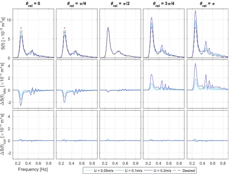
4.2. Uni-directional parametric spectrum

The observed transformation of the parametric spectra is shown in

Fig. 8, along with the deviation in energy density compared to the desired before and after correction. Clearly the same trend is seen as with the regular waves, with larger transformations in the presence of larger currents, and larger wave heights with increasing angle.

Analysing this change in energy density, it can be inferred that although the majority of the change is a result of wave-current interac-tion, there is also significant variation due to reflections, particularly affecting the higher frequencies. The magnitude of these variations are a function of the reduced absorption effectiveness in the presence of larger currents. The reason for this‘spiky’variation at higher frequencies is due to incident and reflected wave components at a given frequency being in or out of phase at the gauge array location.

Regardless of the source of the frequency dependent variation, the corrected deviation shows that the spectrum has been effectively cor-rected using a linear approach in a single iteration. All wave-current-angle scenarios were corrected to give afinal weighted error of less than 3%.

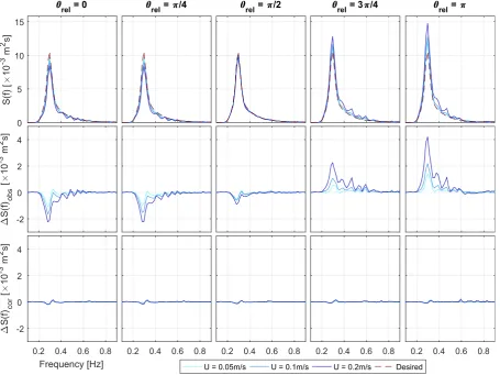
4.3. Non-parametric directional spectrum

Similar to the parametric outputs found in Fig. 8, the frequency spectrum transformation and correction for the non-parametric EMEC derived sea state are shown inFig. 9. Again, only a single iteration was required to achieve these results. Despite this sea state having significant directional spreading associated, similar magnitude of transformation is observed to the parametric case, along with analogous influence of

re-flections. The corrected frequency spectra are also all within 3% of the desired, demonstrating that the linear correction procedure applied to the sub-frequency angular components is just as effective.

Fig. 10shows thefinal corrected sea states output. Frequency spectra along with weighted DSF are shown, for the three velocities andfive relative angles. Thefinal directional spectrum output using the PTPD approach is shown for the base 0.1 m/s case, noting that the 0.05 m/s and 0.2 m/s results appear very similar.

Thefinal sea states re-iterate that the frequency spectra have been effectively corrected for all velocity-angle combinations, and in general so have the directional spectra and mean DSF. Directional errors are larger with increasing current velocity which is clear when assessing the weighted DSF errors. With zero current the weighted DSF error was

Fig. 6.Results for regular waves at nine measured angles to the current direction and three velocities.H0refers to wave height values obtained without the presence of current,

andθ0refers to the input wave angle, known to be correct. Panels show (a) Observed

6.95%, whereas in 0.05, 0.1 and 0.2 m/s current the mean errors over all angles are 13.3%, 14.3% and 18.5% respectively. Although this is a significant increase it is felt that the majority of this is not refraction induced and instead is a product of increased measurement error com-bined with the way the error is calculated. This is discussed further in Section5.3.

5. Discussion

5.1. Observed change in wave height and spectra

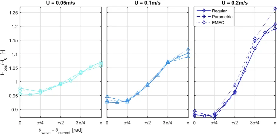
Although the main aim of this work is to demonstrate the effective re-creation of directional spectra with current, one of the interesting

Fig. 7.Observed change in wave height for regular waves at various angles to the current direction, with comparison to theory.

outcomes is the observation of non-collinear wave current interactions. All results show larger wave transformation in the presence of higher current velocities and an increase in wave amplitude with increasing relative angle, as would be expected. The magnitude of the regular wave transformation, however, was much larger than expected, as shown inFig. 7.

The change in wave height (regular or significant) with respect to the current condition was observed to be comparable for each of the sea states. This is shown inFig. 11, and is largely a result of all sea states having similar frequency and steepness values. It may be expected that the directional sea state would have a smaller range in measured wave heights due to different wave components propagating at different rela-tive angles. However, this proved not to be the case, which is clear when assessing the observed wave height for the EMEC sea state in 0.2 m/s current at a relative angle ofπ. The cause of this is unknown, but may be a consequence of reflections causing a net constructive effect over the wave gauge array area. These reflections are dependent on frequency,flow velocity, and relative angle.

As expected from the similar wave height transformations, the spectra also display a larger transformation than predicted by linear theory (Section2). These discrepancies may be a result of tank specific wave generation issues in the presence of a current (discussed further in Sec-tion5.2), so caution must be used before assuming that these results are representative of pure wave-current interaction. Interestingly, however, the same effect has been observed byNwogu (1993); Chakrabarti and Johnson (1995); Guedes Soares et al. (2000). Although this does not resolve the cause of the difference it does suggest that, at least in part, these larger transformations may be a pure wave-current interac-tion effect.

Interestingly, wave height was found to decrease in all cases where the mean wave angle was perpendicular to the current, with a greater reduction at higher velocities. With the current running, water passes through the turning vanes, and wave energy may be lost via the current return path under thefloor. This is analogous to having afinite crest length in open water, with the perpendicular current causing wave crests to‘stretch out’along their length, thus reducing wave height. The the-ories considered assume plane waves with infinitely long crests, so pre-dict no change in wave height with a perpendicular current.

5.2. Assessment of correction procedure

The amplitude correction procedure applied has proven to be effec-tive for all sea states, providing frequency spectrum errors of less than 3% in all cases. Consequently, the resulting wave heights were found to be very close to the desired. For the regular, uni-directional parametric, and non-parametric EMEC sea states, the mean wave height discrepancy over all velocity-angle combinations were found to be 0.27%, 0.42% and 0.91% respectively (maximum errors of 0.67%, 1.11% and 1.38%).

The correction factor, although assumed linear, includes a number of different factors of which the proportional influence remains un-known. Namely:

1. Superposition of wave and currentfields, 2. Energy transfer between wave and currentfields,

3. Increased reflections with larger currents, which is relative to the array location,

4. Spatial variation of current in the tank, and 5. Paddle response to presence of current.

The favourable results show that, although current effects on the wavefield at FloWave are inherently complex and non-linear, the vari-ation in relative wave deformvari-ation as a result of a modest change in input wave amplitude can effectively be approximated as a linear process. This is a useful output from this work, although limits to the validity of this will need to be identified through additional testing with steeper waves and higher current velocities. The wave-current interaction theories do not include all of these factors, which may account for the discrepancies inFig. 7. The linear theory only accounts for thefirst, while the

non-linear theory also partially accounts for the second. Factors 3–5 are fa-cility specific, and thus cannot be dealt with by general theories.

5.3. Measurement of wave directionality

5.3.1. Measurement of component wave angles in current

Component angles are measured using the PTPD approach as imple-mented byDraycott et al. (2016). Each gauge triad provides an estimate of wave angle for each of the frequency components based on the

Fig. 10.Final non-parametric EMEC spectra following correction, at 5 relative angles to current. Top row shows spectral densitySðfÞ, middle row weighted mean directional spreading functionDSFmean, and bottom row directional spectraEðf;θÞfor 0.1 m/s current.

measured phase differences from an FFT. A circular kernel density esti-mate (250 bins) is then applied to the 56 individual triad estiesti-mates in an aim to identify the true incident angle for each component. This approach has been shown to provide very good estimates of incident wave angle without the presence of current, typically identifying the correct angle within π=90. Noting the directional bin widths are π=32 this usually provides good resulting spectral estimates.

In the presence of currents, estimates of wave angle are not so accu-rate. This is partly due to additional measurement uncertainty from a number of sources: run-up on gauges, turbulence, and Vortex Induced Vibration (VIV). The presence of the current also causes inconsistent bending to occur in the gauges meaning the assumed gauge positions are somewhat inaccurate, and importantly wire separations can be variable. Additionally, reflection levels are higher in the presence of currents, which also alter the perceived phases, particularly when the reflections are not opposing the incident components. The cumulative effect of this is increased uncertainty in the angular estimates.

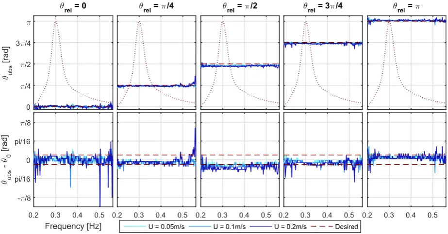
Fig. 12 shows the PTPD angle calculation outputs for the uni-directional parametric spectrum, noting that it is much easier to observe and analyse than the non-parametric directional sea state. It is clear that the overall sea state direction is generally identified well. With directional bin size ofπ=32, a measured deviation of justπ=64 from the desired angle would result in the energy being attributed to a different directional bin for that frequency component. This happens relatively frequently in the presence of current as can be seen inFig. 12, causing apparently large errors to arise through a measurement discrepancy of less than three-degrees. This results in the DSF and Eðf;θÞin Fig. 9

showing significant deviation, even though the underlying errors them-selves are quite minimal. To get an error metric not related to bin size, a net weighted angular error has been defined in Eq. (14), with the observed outputs for both the parametric and non-parametric EMEC sea shown inFig. 13.

θ error¼

P

ðθobs_P;iθ0;iÞAi

Ai

(14)

As refraction levels are expected to be in the order of a few degrees, isolating what is refraction and what is simply increased measurement error has proved difficult. Any significant refraction should, however, manifest itself as a negative weighted angular change inFig. 13for all

non-collinear cases. As there is no clear indication that this is the case, it is assumed that the refraction levels in these tests are low enough that

Fig. 12. Observed wave component angles at different velocities (top) and discrepancy from desired (bottom). Amplitude spectrum shown dotted in top panels to highlight where energy content lies. Spacing between dashed lines in lower panels represents directional bin size.

they do not need to be corrected. If this work was to be extended to tests with larger currents it may be that the refraction cannot be ignored, requiring improvements to the measurement system. This may take the form of stiffer wave gauges (or an alternative measurement system) to reduce vibration and deflection in the presence of current. This would allow the implementation of an iterative procedure to correct for the observed refraction.

5.3.2. Relative performance of PTPD approach

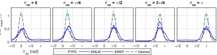
In the presence of a current, the increased measurement errors mean that the PTPD outputs have some uncertainty associated. Although it has been inferred that the actual discrepancy is likely to be small, this still means that the true directional spectrum generated remains unknown. This uncertainty, however, is still significantly smaller than if typical directional spectrum reconstruction methods were used. This is demon-strated inFig. 14, where the DSF outputs for the base 0.1 m/s cases are shown for the PTPD, Extended Maximum Likelihood Method (EMLM) and Extended Maximum Entropy Method (EMEP) approaches. InFig. 14

it appears that other than the EMEP reconstruction at 3π=4, the EMEP and EMLM approaches fail to effectively characterise the DSFs; having a non-zero magnitude for all angles. This is clearly not the case and is likely due to the limitations of these‘curve-fitting’methods trying tofit to small reflections, along with additional reconstruction errors. As there is only significant energy within a range ofπ=4, and the array is in the tank centre (meaning component reflections are opposing incident), there should only be a very small DSF component (1–4% size of incident peak corresponding to 10–20% reflection) opposing the incident, rather than the observed constant energy content.

The poor performance of the EMEP and EMLM approaches in these instances mean that the resulting reconstructions would clearly not be suitable to use as a basis for subsequent directional correction. Despite the PTPD approach reducing errors significantly, identification of refraction effects with these low velocities and wave gauges available is still error prone. It is thought, however, that using this approach with stiffer gauges will prove effective at measuring DSFs accurately in cur-rent, with the additional advantage that component angles have been calculated, and can now inform a correction procedure.

5.4. Application and implications for physical testing

The results of this work demonstrate that site-specific directional spectra can be re-created with current at FloWave. It also highlights the importance of including any currents present when aiming to re-create site conditions, and the value in obtaining measurements of current ve-locity when carrying out resource assessment, or carrying out full scale testing.

When re-creating site conditions for tank testing, including measured or representative currents can help explore the envelope of expected responses. This will in turn provide more insightful and realistic device and mooring loads, including both those incurred through the presence

of the current directly as well as those resulting from the influence of the current on the wavefield. If combined conditions are specified, then the input spectrum will need to be corrected so that the desired spectrum is obtained at the device location, thus appropriately representing the power available. With the current included, the correct wavenumber spectrum will also be obtained, ensuring that wave amplitudes, along with wavelength, steepness and celerity match those at the site.

Due to the significant effect current can have on the perceived power and assumed wavelengths, it is clearly advantageous to measure current velocities when carrying out resource assessment. This is also the case when carrying out full scale testing as it enables true context to be placed on the results. For example, if characterising a WEC perfor-mance byHm0andTe, a device sensitive to wavelength and steepness

will respond very differently in the presence of current despite having comparableHm0–Tevalues (in addition to the available power being

misinterpreted).

The level of sea state complexity generally increases as a concept advances through Technology Readiness Levels (TRLs) (Ingram et al., 2011). Early stage testing is typically limited to regular waves of varying frequency and height before advancing to standard parametric spectra (both long and short crested). The ability to produce combined wave-current sea states, especially with non-parametric spectra, will usually apply more to devices at advanced TRLs where a particular deployment site has been identified. As such, this ability to produce site-specific combined sea states has the potential to extend and com-plement established development paths.

6. Conclusions

A site-specific non-parametric directional spectrum has been obtained from EMEC, and re-created at 1:26 scale at the FloWave Ocean Energy Research Facility with current velocities of 0.05, 0.1 and 0.2 m/s (rep-resenting 0.5, 1 and 2 knots full scale). The studies conducted on complex directional wavefields in combination with currents within the FloWave Ocean Energy Research Facility resulted in the following mainfindings:

The transformation of waves by current has been shown to have a significant impact on both the true wave power and steepness, and on that which may be assumed without knowledge of the currentfield. If the current present at the site is not included in tank testing, incorrect power and wavenumber spectra will be generated, and test results will not be representative of real site conditions.

An empirical correction procedure has been used to correct this sea state, along with equivalent regular waves and uni-directional para-metric spectrum, in the presence of currents from multiple relative angles. The linear correction procedure applied proved effective after a single iteration, providing corrected frequency spectra all within 3% of the desired, and wave heights normally within 1%. Refraction ef-fects were found to be minimal at the velocities tested. Although angle estimates prove to be error prone in current, the PTPD approach

provides much improved outputs over either the EMLM or EMEP methods.

In this process, non-collinear wave-current interactions were observed for each of the wave cases. The measured wave trans-formation was larger than expected from theory, which may partially be facility specific effects resulting from the method of generating currents and absorbing waves at FloWave.

Acknowledgements

The authors would like to thank the Energy Technologies Institute and RCUK Energy programme for funding this research as part of the IDCORE programme (EP/J500847/1), the UK EPSRC for funding the FloWave facility (EP/I02932X/1), and the European Marine Energy Centre for providing buoy data for the sea state replication work.

References

ABP MER, 2012. Pentland Firth and Orkney Waters Strategic Area : Marine Energy Resources. Tech. Rep. November, The Crown Estate.

Baddour, R.E., Song, S., 1990. On the interaction between waves and currents. Ocean Eng. 17, 1–21.

Chakrabarti, S., Johnson, J., dec 1995. Random wave-current interaction–theory and experiment. In: Proceedings of the 19th International Conference on Ocean, Offshore and Arctic Engineering (OMAE2000).

Draycott, S., Davey, T., Ingram, D.M., Day, A., Johanning, L., 2016. The SPAIR method: isolating incident and reflected directional wave spectra in multidirectional wave basins. Coast. Eng. 114, 265–283.

Draycott, S., Davey, T., Ingram, D.M., Lawrence, J., Day, A., Johanning, L., 2015. Applying site-specific resource assessment : emulation of representative EMEC seas in the FloWave facility. In: Proceedings of the 25th International Offshore and Polar Engineering Conference.

Draycott, S., Davey, T., Ingram, D.M., Lawrence, J., Johanning, L., Day, A., Steynor, J., Noble, D.R., 2014. Applying site specific resource assessment: methodologies for replicating real seas in the FloWave facility. In: Proceedings of the 5th International Conference on Ocean Energy, Halifax, Canada.

Earle, M., 1996. Nondirectional and Directional Wave Data Analysis Procedures. NDBC Tech. Doc. 96 002 (January).

Esteva, D., 1976. Wave direction computations with three gage arrays. In: Coastal Engineering Proceedings.

Fernandes, A.A., Sarma, Y.V.B., Menon, H.B., 2000. Directional spectrum of ocean waves from array measurements using phase/time/path difference methods. Ocean Eng. 27 (4), 345–363.

Guedes Soares, C., Rodriguez, G., Cavaco, P., Ferrer, L., 2000. Experimental study on the interaction of wave spectra and currents. In: Proceedings of the 19th International Conference on Ocean, Offshore and Arctic Engineering (OMAE2000).

Hashemi, M.R., Neill, S.P., Davies, A.G., Lewis, M.J., 2014. The implications of wave-tide interactions in marine renewables within the UK shelf seas. In: Proceedings of the 2nd International Conference on Environmental Interactions of Marine Renewable Energy Technologies (EIMR2014). No. May 2014. Stornoway, Scotland.

Hedges, T.S., Anastasiou, K., Gabriel, D., 1985. Interaction of random waves and currents. J. Waterw. Port, Coast. Ocean Eng. 111 (2), 275–288.

Holmes, B., Nielsen, K., 2010. Guidelines for the Development&Testing of Wave Energy Systems. Tech. Rep. June, Hydraulics Maritime Research Centre, UCC, Cork, Ireland. Ingram, D., Wallace, R., Robinson, A., Bryden, I., 2014. The Design and Commissioning of

the First, Circular, Combined Current and Wave Test Basin.

Ingram, D.M., Smith, G.H., Bittencourt Ferreira, C., Smith, H.C.M., 2011. EquiMar protocol II.A tank testing. In: Protocols for the Equitable Assessment of Marine Energy Convertors. Edinburgh, Ch. 3.3.

Jonsson, I., 1990. Wave-current interactions. In: LeMehaute, B., Hanes, D.M. (Eds.), The Sea, Ocean Engineering Science, vol. 9. Wiley-Interscience publications, New York, pp. 65–120. Ch. 7.

Kemp, P.H., Simons, R.R., apr 1982. The interaction between waves and a turbulent current: waves propagating with the current. J. Fluid Mech. 116 (-1), 227–250. Kemp, P.H., Simons, R.R., apr 1983. The interaction of waves and a turbulent current:

waves propagating against the current. J. Fluid Mech. 130, 73–79. Mankins, J.C., 1995. Technology Readiness Levels. White Paper, April, 4–8.

Miles, M.D., Funke, E.R., 1989. A Comparison of Methods for Synthesis of Directional Seas. Noble, D.R., 2017. Combined Wave-current Scale Model Testing at FloWave. Ph.D. thesis.

University of Edinburgh.

Noble, D.R., Davey, T., Smith, H.C.M., Kaklis, P., Robinson, A., Bruce, T., 2015. Characterisation of spatial variation in currents generated in the FloWave Ocean energy research facility. In: Proceedings of the 11th European Wave and Tidal Energy Conference, Nantes, France. Nantes, France.

Nwogu, O., jun 1993. Effect of steady currents on directional wave spectra. In: Proceedings of the 12th International Conference on Offshore Mechanics&Arctic Engineering (OMAE1993). ASME, Glasgow, UK.

Pascal, R., 2012. Quantification of the Influence of Directional Sea State Parameters over the Performances of Wave Energy Converters.

Peregrine, D.H., 1976. Interaction of waves and currents. In: Advances in Applied Mechanics, Vol. 16. Elsevier, pp. 9–117.

Plant, W., 2009. The ocean wave height variance spectrum : wavenumber peak versus frequency peak. J. Phys. Oceanogr. 1, 2382–2383.

Robinson, A., Ingram, D., Bryden, I.G., Bruce, T., jan 2015. The generation of 3Dflows in a combined current and wave tank. Ocean Eng. 93.

Saruwatari, A., Ingram, D.M., Cradden, L., nov 2013. Wave-current interaction effects on marine energy converters. Ocean Eng. 73, 106–118.

Smith, J.M., 1997. Coastal Engineering Technical Note One-dimensional Wave-current Interaction (CETN IV-9). Tech. rep., US Army Engineer Waterways Experiment Station, Coastal Engineering Research Center, Vicksburg, MS.

Thomas, G.P., 1981. Wave-current interactions: an experimental and numerical study. Part 1. Linear waves. J. Fluid Mech. 110 (1981), 457.