City, University of London Institutional Repository
Citation
: Jones, P. R. ORCID: 0000-0001-7672-8397 (2018). The development of
perceptual averaging: Efficiency metrics in children and adults using a multiple-observation sound-localization task. Journal of the Acoustical Society of America, 144(1), pp. 228-241. doi: 10.1121/1.5043394This is the accepted version of the paper.
This version of the publication may differ from the final published
version.
Permanent repository link:
http://openaccess.city.ac.uk/20359/Link to published version
: http://dx.doi.org/10.1121/1.5043394
Copyright and reuse:
City Research Online aims to make research
outputs of City, University of London available to a wider audience.
Copyright and Moral Rights remain with the author(s) and/or copyright
holders. URLs from City Research Online may be freely distributed and
linked to.
TITLE
The development of perceptual averaging: efficiency metrics in children and adults using a multiple-observation sound-localization task
RUNNING TITLE
The development of perceptual averaging
AUTHORS
Pete R. Jones
Institute of Ophthalmology, University College London (UCL), 11-43 Bath Street, London EC1V 9EL;
ABSTRACT [Max 200 Words; Currently 194]
This study examined the ability of older children to integrate spatial information across 1
sequential observations of bandpass noise. In Experiment I, twelve adults and twelve 8—14-year-2
olds localized 1—5 sounds, all presented at the same location along a 34o speaker array. Rate of
3
gain in response precision (as a function of N observations) was used to measure integration
4
efficiency. Children were no worse at localizing a single sound than adults, and - unexpectedly --5
- were no less efficient at integrating information across observations. Experiment II repeated the 6
task using a Reverse Correlation paradigm. The number of observations was fixed (N = 5), and the
7
location of each sound was independently randomly jittered. Relative weights were computed for 8
each observation interval. Distance from the ideal weight-vector was used to index integration 9
efficiency. The data showed that children were significantly less efficient integrators than adults: 10
only reaching adult-like performance by around 11 years. The developmental effect was small, 11
however, relative to the amount of individual variability, with some younger children exhibiting 12
greater efficiency than some adults. This work indicates that sensory integration continues to 13
mature into late childhood, but that this development is relatively gradual. 14
I. INTRODUCTION
15
On simple psychophysical tasks, older children often perform as well as adults1. For example, the
16
ability to discriminate the frequency of two tones is adult-like by around 8 years of age2, while the
17
ability to localize a single sound matures by around 6 years3. In everyday life, however, we are
18
often presented with complex scenes, containing multiple sources of stochastic information. In 19
such circumstances, perceptual judgments are limited not only by our ability to encode individual 20
stimuli, but also by our ability to integrate multiple observations together, to make a single, 21
overall decision. 22
Outside of audition, children’s ability to integrate information across multiple sensory ‘channels’ 23
is believed to remain immature until late childhood. For example, children up until 10 – 12 years 24
have been shown to fixate disproportionately on a single modality in multisensory tests of 25
navigation4, visuohaptic size discrimination5, and audiovisual stimulus detection6 (for reviews,
26
see [7,8]). While within vision, the ability to combine different stimulus features (e.g., texture and
27
stereoscopic disparity) to judge depth has been found to mature only by around 11-12 years9,10.
28
Within audition, the developmental time course is unknown. However, there is clear evidence of 29
suboptimal integration in early childhood. For example, Allen, Jones, & Slaney (1998)11 observed
30
that adults exhibited a substantial benefit (~8 dB) on a tone-in-noise detection task when the 31
target was positioned spectrally off-center. In contrast, preschool children (4--5 years) gained no 32
such benefit, indicating that they were unable to exploit both pitch and level cues. 33
It is also striking that where the development of sensory integration has been studied, it is often 34
limited to tasks involving only two channels of information. And it is known that as the number of 35
channels increases, even adults’ performance start to deviates from the ideal12–14 -- possibly due
36
to constraints on memory or attention. This raises the possibility that, in arguably more realistic 37
scenarios, where more than two sources of information are present, children may not be any 38
poorer than adults at integrating information. Indeed, one recent study by Leibold and Bonino15
suggests this might be the case. There, it was found that children’s detection thresholds for a tone 40
in noise improved progressively the more the target was repeated (N = 1 to 5), and the rate of
41
improvement did not differ significantly between children and adults. 42
The purpose of the present study was to quantify the ability of older children (aged 8 – 14 years) 43
to integrate sequential auditory signals, and to determine at what age this ability matures. To 44
quantify efficiency, we used a ‘multiple observation’12 perceptual averaging task. On each trial, the
45
listener was presented with a sequence of sounds, all centered on a single location along the 46
azimuth (location randomized between trials). The listener’s task was to listen to all N sounds,
47
before judging the (single) source location. Two separate techniques were used, in two 48
independent experiments, to estimate the efficiency with which listeners combined the N
49
observations to form a single estimate of location. Each experiment is reported more fully in turn, 50
but in brief: 51
Experiment I measured integration efficiency using a relatively old method based on the rate of 52
gain in response precision as a function of N observations. During the experiment, N was varied
53
randomly between 1 to 5. Within a single trial, all N sounds were presented at the exact same
54
location. This meant that every observation was equally informative, and the response precision 55
of the ideal observer are predicted to improve at a rate of √𝑁16. To the extent that listeners failed
56
to integrate additional observations, their response precision would improve at a lesser rate. The 57
rate of gain provided an index of integration efficiency. 58
Experiment II used a more modern measure integration efficiency based on Reverse Correlation. 59
The number of observations was fixed at N = 5 and the location of each sound was randomly
60
jittered between observations. Each of the five observations therefore predicted a slightly 61
different response. The relative correlation between the listener’s actual responses, and the 62
relative weight given to each observation. To the extent that the listener utilized all five 64
observations, equal weight should be given to each. Conversely, a suboptimal integrator would 65
over-weight some temporal intervals, and under-weight others. The similarity of the observed 66
weights vector to the ideal provided an index of integration efficiency. 67
Previous studies have used variants of both methods in adults12,13. These studies have shown that
68
adults are effective but sub-optimal integrators: deriving a measurable benefit from every 69
additional information channel, but less benefit than would be predicted by an ideal observer. The 70
novel aspect of this present work was the application of these methods to children. It was 71
therefore unknown how they would perform. In particular, it was unknown: how children’s 72
efficiency compared to adults, and which (if any) of the N observations children would fail to
73
exploit. 74
75
[image:6.595.49.548.418.627.2]76
FIG 1. Stimuli andtest apparatus for both experiments. (A) The listener’s task was to locate the [single] source 77
location of N noise bursts. Stimuli were presented along the azimuth, using 18 speakers distributed uniformly at 2° 78
intervals along a 34° arc. Eighty LEDs arranged below the speakers were used for response-input, feedback, and 79
fixation-cuing; (B) Each observation consisted of a 200 ms band-passed noise burst (1 octave bandwidth), centered
80
at 1 kHz. (C) Each trial consisted of N observations (shown here: N = 5), presented sequentially with an inter-81
stimulus interval of 100 ms. (D) In Experiment I, N varied from 1 to 5, between blocks, in random order. Within each 82
trial, the target location (thin red vertical line) varied randomly, and all sounds (thick blue lines) were presented at 83
the target location (shown here: target = -1.25°). (E) In Experiment II, N was fixed at 5, and the location of each sound 84
was randomly distributed around the target location, based on independent samples from a truncated-gaussian 85
II. EXPERIMENT I: Relative gain in response precision as a function of N observations
87
The goal of Experiment I was to quantify integration efficiency in children and adults, using the 88
relative gain in response precision as the number of observations, N, increased. The logic of this
89
method is derived from basic Signal Detection Theory12, and is described more fully elsewhere12.
90
In brief: let us assume that the response to a single sound is determined by some putative 91
‘internal response’, which is a scalar value proportional to the observed stimulus value, plus a 92
sample of additive noise (i.e., due to random error due to intrinsic neuronal, physiological, or 93
cognitive variability): 𝑥 +. And let us model the additive noise term as a zero-mean Gaussian
94
variable, – a choice that is mathematically expedient, but which in the present case
95
is also supported by the empirical data (see Fig S1 in the Supplementary Material17). If we
96
operationalize response precision as the reciprocal of the standard deviation of the observed 97
response error, 1
𝜎, then response precision in the single stimulus condition is determined purely
98
by the standard deviation (‘magnitude’) of the internal noise, σ𝑖𝑛𝑡:
99
(Eq 1)
When presented with multiple, equally-reliable observations, the ideal observer will mean-100
average the N internal responses: ∑𝑁𝑖=1[𝑥𝑖 +𝑖]. The decision variable will therefore be the mean
101
of N normally distributed random variables, which is itself a normally distributed random
102
variable with a mean of 𝑥̅ and a standard deviation of 𝜎 √𝑁⁄ . We would therefore expect the
103
response precision of an ideal observer to improve at a rate of √𝑁 (for more detailed theory, see 104
References [12,16]).
105
Conversely, a listener who used only some proportion, k, of the additional information, would gain
106
(Eq 2)
For example, when k = 0, precision with N observations would be the same as precision with one 108
observation (no improvement). As k increases towards 1, the rate of relative improvement 109
becomes closer to the ideal: √𝑁. Thus, if N = 3 and k = 0.5, precision would be~1.41 (√2) times 110
greater than precision given a single observation, while if k = 1 precision would improve by ~1.73 111
(√3). 112
By combining Eqs 1 and 2 it can be seen that 𝜎𝑁⁄𝜎1 (the ratio of response precision given N
113
observations, to precisiongiven one observation only) is determined solely by the single 114
unknown parameter k, together with the experimentally controlled parameter N:
115
(Eq 3)
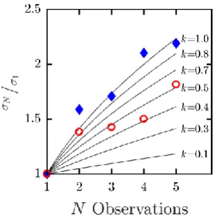
Thus, by plotting empirical values of 𝜎𝑁⁄𝜎1 as a function of N, the best-fitting value of k
116
(proportion of observations used) can be estimated. This is illustrated graphically in Figure 2, 117
which shows individual data for two individuals, superimposed against isobars for various values 118
of k, ranging from no integration (k = 0) to full integration (k = 1). By inspection, it can be seen
119
that one listener (red circles) used only ~50% of the additional information, while a second 120
listener (blue diamonds) was a near-optimal integrator (~100%). In practice, values of k were
121
estimated numerically by finding the value of k that minimized the least-square error between Eq
122
FIG 2. Experiment I: The determination of k (proportion of observations used),
124
using five successive observations of a 1-octave noise burst. Black lines are 125
isobars denoting the rate of gain predicted as integration varies from k = 0 (no 126
integration) to k = 1 (full integration. Red circles and blue diamonds are data 127
from two individual listeners. 128
A. Experimental Methods 130
1. Task Overview 131
As illustrated in Figure 1, the task wasto localize the [single] source of N noise bursts
132
(‘observations’), where N varied from 1 to 5 between blocks (random order). The N observations
133
were presented sequentially at a random location along a 34o array of loudspeakers, which was
134
arranged in a frontal arc around the participant. After all N observations, the participant made a
135
single response, by using a rotary dial to position a light at the perceived sound-source location. 136
Participants were encouraged to “listen carefully to all of thesounds without moving your head,
137
before deciding where the sounds were coming from”. 138
2. Participants 139
Participants were 12 normal hearing children, aged 7.9 – 13.9 years (µ = 11.0, σ = 2.0), and 12
140
normal hearing adult controls, aged 18 – 30 years. Adults were recruited through the UCL 141
Psychology Subject Pool (‘SONA’), and received £7.5/h compensation. Children were recruited 142
through the UCL Child Vision Lab volunteer database, and received certificates and small toys. 143
Written consent was obtained from all participants (adults) or the responsible caregiver 144
(children). Children themselves also gave written assent. The experiment was conducted in 145
accordance with UCL Research Ethics Committee approval (#7611/001). 146
3. Stimuli & Apparatus 147
Each stimulus consisted of N band-pass noise bursts separated by inter-stimulus intervals of 100
148
ms. Each noise burst was 200 ms in duration, including 10 ms cos2 on/off ramps (see Fig 1B-C).
149
Each burst was independently randomly generated by filtering white Gaussian noise through a 150
pair of second-order Butterworth band-pass filters, with cut-offs 1-octave either side of 1 kHz 151
(i.e., 0.5 kHz High Pass, 2 kHz Low Pass). Stimuli were presented over loudspeakers, at an 152
uniform distribution, and was designed to prevent loudness inadvertently becoming a location 154
cue (e.g., due to errors in calibration, or systematic differences in room-acoustics). 155
The exact choice of stimulus is not expected to have influenced the ability of children or adults to 156
integrate observations. However, the bandwidth of the signal (1 octave) was significant from a 157
practical perspective. The ability of listeners to localize sounds stimuli declines precipitously for 158
narrower bandwidths18, and it was observed during piloting that listeners often became
159
unmotivated when presented with narrowband noise or pure tones. In such circumstances, 160
listeners were also liable to be influenced in their responses by a priori information (i.e., the
161
visible extent of the speaker ring). Very wideband stimuli were also deemed inappropriate, as, 162
consistent with previous findings18, some pilot listeners performed close to ceiling when
163
presented with a single burst of white noise at certain locations. The center frequency of the 164
stimulus (1 kHz) meant that the signal contained both ITD and ILD cues. However, the choice of 165
center frequency is unlikely to have affected observed behavior substantially, as the ability to 166
localize broadband stimuli along the azimuth is largely independent of center frequency for 167
bandwidths of 1 octave or greater18.
168
Stimuli were presented using an array of eighteen speakers (Visaton SC 5.9; Visaton GmbH, Haan, 169
Germany), which were positioned symmetrically, equidistant from the listener. The speakers were 170
uniformly-spaced in 2° intervals along a circular arc spanning ±17° either side of the listener’s 171
midline [Fig 1A]. Each speaker was located 2.87m from the listener. To allow sounds to be located 172
continuously anywhere along the 34° arc, Vector Distance Panning was used to interpolate 173
between speakers19. Panning was used to ensure that the distribution of target locations was as
174
close to gaussian-distributed as possible, and also to minimize the possibility that listeners might 175
learn the N discrete speaker locations. The use panning may have introduced a small amount of
176
previous studies in which panning was not employed (see General Discussion). An acoustically 178
transparent curtain was arranged in front of the speakers, to prevent listeners from assuming 179
that sounds were only ever located at the 18 discrete speaker locations. 180
Stimuli were digitally synthesized in MATLAB v7.4 (2012a, The MathWorks, Natick, MA) using a 181
sampling rate of 44.1~kHz and 24-bit quantization. Stimulus presentation was controlled using 182
the Psychophysics Toolbox v320 ASIO wrapper (Steinberg Media Technologies, Hamburg).
Digital-183
to-analogue conversion was carried out by a Focusrite Saffire PRO 40 (Focusrite plc, UK) external 184
sound card (channels 1 to 10), and by an Ultragain Digital ADA8000 (Behringer GmbH, Willich, 185
Germany) ADAT interface (channels 11 to 18). Audio signals were amplified using nine Lvpin Hi-186
Fi 2.1 stereo amps (Lvpin Technology Co. Ltd, Suzhou, China). Output levels were equalized using 187
an Investigator 2260 sound level meter (Bru el & Kjær, Nærum, Denmark), and were adjusted to 188
ensure no noticeable differences in intensity or timbre. 189
Directly below the speakers was an array of 80 light-emitting diodes (12 mm diffused digital LED 190
pixels; Adafruit Industries, New York, New York, USA), distributed uniformly between ± 19.75°, in 191
intervals of 0.5°. The LEDs were used to provide: (i) a central fixation-target prior to each trial, 192
(ii) post-trial feedback on the true target locations, and (iii) the means by which observers 193
responded (see Procedure, below). An Arduino Uno microcontroller (SmartProjects, Strambino, 194
Italy) was used to interface between the control computer and the LED pixels (see Reference [21]).
195
When making responses, the listener controlled which one of the 80 LEDs was illuminated by 196
rotating a dial (PowerMate USB; Griffin Technology, Nashville, Tennessee, USA). The participant 197
used a keystroke to indicate when done, at which point their response was logged. 198
With both children and adults, the experimenter was present throughout testing, to provide 199
(generally their parent), who sat outside the child's field of vision and who was asked to remain 201
silent during testing. 202
4. Procedure 203
Each trial commenced with a 660 ms visual fixation target, during which the two central LEDs 204
(±0.25°) were illuminated bright red. N successive 200 ms noise bursts were then presented at
205
the target location, separated by inter-stimulus intervals of 100 ms. The target location was 206
randomly selected on each trial, using a uniform distribution between ± 16.75°, rounded to the 207
nearest 0.5° to ensure that the target always fell directly above one of the LEDs (i.e., to ensure 208
accurate responses and veridical feedback). In instances where the target fell between two 209
speaker locations, panning was used to present the stimulus, as described above (Stimuli & 210
Apparatus). 211
Following stimulus presentation, the listener responded by ‘pointing’ to the perceived sound 212
source location. To do this, one of the two central LEDs was randomly selected and was 213
illuminated white. The listener was then given unlimited time to ‘move’ this light to the perceived 214
sound-source location, using a rotary dial to control which of the LEDs was illuminated. Feedback 215
was then given in the form of a green LED light, which was presented at the target location for 216
660 ms. 217
The test session consisted of 250 trials, divided equally between five conditions: N = {1, 2, 3, 4, 5}.
218
Each condition was tested in a separate block of 50 trials, and the order of the blocks/conditions 219
was randomized between listeners. After each block, the listener was given the opportunity to 220
take a short break, as required. Each listener completed a single session, which lasted 221
approximately 60 minutes (including consenting, practice, and breaks). 222
Before the test trials, each listener completed five practice trials. These trials were identical to the 223
test trials, and were all drawn from the N = 3 condition. During this period, the listener was
encouraged to listen carefully to all the sounds, before deciding where [all] the sounds were 225
coming from. 226
B. Results 227
Figure 3 shows mean response precision for adults and children. To analyze these data, a 5x2 228
mixed ANOVA was performed with a within-subject variable of NOBSERVATIONS (5 levels: N = 1--5),
229
and a between-subject variable of AGE (2 levels: children, adults). There was no significant main
230
effect of AGE [F(2,22) = 1.37, p = 0.255, n.s.], indicating that children were no less precise than adults
231
in terms of their overall localization ability (although, prima facie, a possible trend towards higher
232
precision in adults is apparent in Fig 4). In particular, an independent-samples t-test indicated
233
that children were not significantly less precise than adults in the N = 1 condition [t22 = 1.38, p =
234
0.183, n.s.]. 235
However, there was a clear main effect of NOBSERVATIONS [F(4,88) = 7.14, p < 0.001], indicating that
236
precision improved as the number of observations increased. This implies that at least some
237
integration was taking place. Accordingly, precision in the N = 5 condition was significantly higher
238
than in the N = 1 condition, both for children [Paired t-test: t11 = 3.80, p = 0.003], and adults [t11 =
239
3.79, p = 0.003]. There was no interaction between AGE and NOBSERVATIONS [F(4,88) = 0.20, p =
240
0.937, n.s.], suggesting that the rate of improvement, and therefore the amount of integration, was
241
243
FIG 3. Experiment I:Group-mean [± 1 S.E.] response variability for 244
children (red crosses) and adults (blue circles), shown as a function 245
of N Observations. Lower values denote greater precision. For the 246
ideal observer, imprecision would be expected to decrease at a rate 247
of √𝑁. 248
249
250
251
252
253
254
255
The foregoing implies that both children and adults integrated information from at least two 256
observations (in the nomenclature of Boyaci and colleagues22, adults and children were both
257
‘effective integrators’). However, these analyses do not allow us to quantify the relative efficiency 258
of children and adults. 259
To formally assess integration efficiency, we computed 𝜎𝑁⁄𝜎1 and estimated k (proportion of
260
observations used), using the procedure described in the Methods. Results are shown for 261
individuals in Figure 4. By inspection, there was substantial inter-individual variability, but no 262
systematic difference between children and adults. This was confirmed statistically using a Mann-263
Whitney U test, which found no significant difference in efficiency, k, between children and adults
264
[U = 148, Z = -0.09, p = 0.931]. In short, neither age group appeared better at integrating sensory
265
information [Fig 5]. 266
A Wilcoxon Signed-Rank test indicated that, on average both children [p < 0.001] and adults [p <
267
0.001] deviated significantly from the ideal observer (dashed lines in Figs 4 & 5), indicating that 268
both were suboptimal, and failed full use of the additional information. However, it can be seen in 269
Figure 4 that there were individual exceptions, with some adults and some children performing 270
272
273
FIG 4. Experiment I:Value of 𝜎𝑁⁄𝜎1 for all individuals. Solid lines represent least-square fits of Eq 3 to the data, 274
from which estimates of the integration index, k, were derived (see Fig2 for details). Dashed lines show the ideal rate 275
of gain (√𝑁). Individual children have been ordered by age (ascending). 276
[image:16.595.52.519.94.424.2]277
FIG 5. Experiment I:Group-mean [± 1 S.E.] integration efficiency for children and adults (same data as Fig 4). 278
C. Interim Discussion
280
The results from Experiment I showed that both children and adults are able to integrate 281
information across multiple, sequential observations. However: (i) both children and adults were 282
suboptimal, and on average exhibited lower integration efficiency than the ideal observer 283
(although substantial individual variability was observed). Furthermore, and contrary to 284
expectations: (ii) children were, on average, no less efficient at integrating information than 285
adults. 286
The fact that integration efficiency was relatively low in adults stands in apparent contradiction 287
to the wider ‘cue-combination’ literature, where sensory integration in adults is generally 288
reported to be near-optimal (for a review, see 23). However, findings of near-optimality are
289
generally predicated on tasks involving only two channels of information. In contrast, when, as in 290
the present task, larger numbers of channels are presented sequentially, studies in both 291
vision13,14 and audition12 have, like the present work, tended to report effective but suboptimal
292
integration. 293
That children’s localization precision improved at the same rate as adults is consistent with a 294
study by Leibold and Bonino (2009)15, where children’s detection thresholds for a repeated-tone
295
in noise were found to improve at the same rate as adults (see Introduction). Furthermore, the 296
pattern of results observed in Figure 4 are also reminiscent of data from He, Buss, & Hall 297
(2010)24, in which children were asked to detect brief pure tones embedded in a continuous
298
bandpass noise. As the duration of the target tone increased, detection thresholds improved. And 299
although thresholds were consistently poorer for children than adults, the rate of improvement 300
was similar for younger children (5 – 7.5 years), older children (7.5 – 10 years) and adults. The 301
absence of any developmental effects in the present experiment were, nonetheless, unexpected, 302
given the overwhelming consensus in the wider developmental literature that sensory integration 303
remains immature until ~11 years7–10.
The conclusions of Experiment I are, however, open to question. To see why, note that by inferring 305
efficiency from the relative gain in response precision, we are assuming, implicitly, that all 306
internal noise is occurs ‘early’ in the encoding process, in the sense that it arises independently in 307
the peripheral auditory system, before any sensory observations are integrated, and so will 308
cancel-out across repeated observations25. In contrast, there are many potential sources of
309
response imprecision that are irreducible, and liable not to cancel-out across observations. For 310
example, motor noise, memory decay, key press errors, variations in response criterion, sensory 311
noise that is correlated across observations, interference between sensory observations (e.g., 312
masking), and/or difficulties in mapping between auditory (stimulus) space and visual 313
(response) space, may all add noise to the listener’s responses, and do so in a way that does not 314
decrease with N (or may even increase). Of these, some potential sources of irreducible noise can
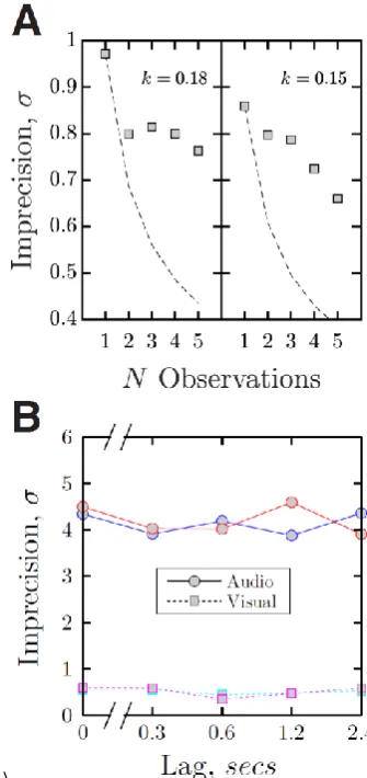
315
be discounted by simple control experiments. For instance, when the experiment was repeated 316
using a visual location cue, overall imprecision was greatly reduced, but continued to decline as a 317
function of N (Fig 6A). This demonstrates that irreducible motor noise is unlikely to be primary
318
limiting factors in the main experiment. Similarly, in a small number of adult controls, 319
imprecision was found not to vary significantly when the lag between a single stimulus and 320
response was systematically increased, either when using a visual (Fig 6B squares) or auditory 321
(Fig 6B circles) stimulus. This suggests that simple memory-decay is also unlikely to be a limiting 322
\ 324
FIG 6. Experiment I control data, from six additional adults. These controls did not participant in the main 325
experiment and were naï ve to the task (A) Data from a visual localization task. The task was identical to the main 326
experiment, except that the N noise burst were replaced with N pulses of white light. As in the main experiment, 327
indices of integration efficiency, k, were computed using Eq 3. The values of k are comparable with those for the main 328
auditory task (Figures 4 & 5). (B) Control data for an N=1 localization condition in which a temporal lag was 329
interposed between stimulus presentation and the participant’s response. Participants were instructed to keep 330
fixating centrally until the response light appeared. Stimuli consisted of either sounds (circles) or lights (squares). 331
Each colored line represents a different observer. 332
To see why irreducible is problematic, note that without the common/convenient assumption 333
that all internal noise is reducible, Equation 2 becomes: 334
(Eq 4)
where 𝜎𝑖𝑛𝑡−𝑟 and 𝜎𝑖𝑛𝑡−𝑖𝑟 are the reducible and irreducible internal noise components,
335
respectively. It follows that Equation 3 becomes: 336
The key point to note is that, unlike Equation 3 (which was used to fit the data in Figures 4 and 5), 337
the internal noise terms in Equation 5 no longer cancel out. The ratio 𝜎𝑁⁄𝜎1 therefore no longer
338
provides an unambiguous measure of integration efficiency, k. Thus, with the model expressed by
339
Equation 5, Listener A may show a greater rate of improvement than Listener B either because
340
Listener A is a more efficient integrator (𝑘𝐴 > 𝑘𝐵), or because a greater proportion of Listener B’s
341
internal noise is irreducible ([𝜎𝑖𝑛𝑡−𝑖𝑟
𝜎𝑖𝑛𝑡−𝑟]𝐴 < [
𝜎𝑖𝑛𝑡−𝑖𝑟
𝜎𝑖𝑛𝑡−𝑟]𝐵). 342
The two key corollaries of this is that we cannot be sure that children are as efficient as adults 343
(i.e., since the proportion of irreducible noise may change with age), and we cannot be sure that 344
individual listeners --- either children or adult --- were in fact integrating suboptimally. To the 345
extent that internal noise is irreducible, listeners may be better integrators than the results of 346
Experiment 1 suggest, and the estimates of k reported in Figure 4 and 5 are only lower bounds on
347
integration efficiency. 348
One way to address the problem of irreducible noise is to explicitly introduce additional external 349
noise that we know to be reducible. For example, Swets et al (1959)12 performed a
multiple-350
observation tone detection task analogous to the localization task reported here. They similarly 351
found that adult performance improved as a function of N, and that the rate of gain was relatively
352
small. Notably though, they also ran a second condition in which independent samples of external 353
noise were added to each observation. In that case, the rate of gain improved markedly, and was 354
close to optimal (√𝑁) for most listeners. This suggests that if Experiment I were repeated with 355
external noise added, estimates integration efficiency might increase, and may start to differ 356
between children and adults. Furthermore, since any external noise is directly observable, it also 357
becomes possible to perform trial-by-trial (‘molecular’26) analyses, to determine which
358
possible to characterize not just whether, but in what way integration is suboptimal. This is the 360
approach taken in Experiment II. 361
III. EXPERIMENT II: Relative decision weights using Reverse Correlation
362
The goal of Experiment II was to again quantify integration efficiency in children and adults. This 363
time, however, external noise was added to each observation, and a Reverse Correlation 364
technique was used to estimate each listener’s decision strategy. 365
The Reverse Correlation methodology is described in detail elsewhere26–28, and has been used
366
previously in adults to study integration of sequentially presented visual stimuli13,14. In brief: just
367
as in Experiment I, N noise bursts were presented on each trial, and the listener was asked to
368
make a single judgment of location. However, the location of each individual noise burst was 369
independently randomly jittered prior to presentation, such that each observation predicted a 370
slightly different response (Fig 1E). By comparing the listener’s trial-by-trial responses 371
(irrespective of their accuracy) to the predictions of the various observations, one can estimate 372
the relative degree to which the listener attends-to/relies-upon each observation. In practice, this 373
procedure was carried out in the present study using a multiple regression model27 (MATLAB’s
374
GLMFIT routine). 375
The result of this analysis is a vector of estimated relative weights, 𝜔𝑒𝑠𝑡, where the ith weight
376
indicates the listener’s relative reliance on the ith observation. By convention we shall normalize
377
this vector such that the absolute magnitudes sum to 1. For example, a listener who only used the 378
first observation would exhibit relative weights of 𝜔𝑒𝑠𝑡 = [1 0 0 0 0]. Conversely, when, as in the
379
present case, all 5 observations are equally informative, the ideal weight vector, 𝜔𝑖𝑑𝑙, is: [0.2 0.2
380
The deviation of the observed weights, 𝜔𝑒𝑠𝑡, to the ideal, 𝜔𝑖𝑑𝑙, provides an index of integration
382
efficiency, 𝜂𝜔, which we can formalise in terms of root-mean-square error29:
383
(Eq 6)
Thus, 𝜂𝜔 = 1 represents perfect efficiency, and lower values indicate a progressive loss of sensory
384
information. Note that this integration index is not directly comparable to the value k, reported
385
previously in Experiment I, although conceptually both are intended to capture the degree to 386
which listeners are able to exploit multiple observations. 387
Crucially, the external noise was sampled independently for each observation, and so would 388
cancel out across observations. This guaranteed that listeners would be more precise when 389
integrating across observations, thereby swamping the effects of any irreducible internal noise. 390
Furthermore, with this method of analysis, some forms of irreducible noise, such as motor error, 391
are largely partialled out from the estimate of integration efficiency, since they add noise to the 392
final response, but in a way that would not be expected to affect the estimated weight-vector, 𝜔𝑒𝑠𝑡
393
(i.e., motor noise would not systematically bias responses towards any single observation 394
interval). 395
A. Experimental Methods 396
1. Task, Stimuli, Apparatus & Procedure 397
The task was identical to Experiment I, with two exceptions. Firstly, the number of observations 398
was fixed at N = 5 for every trial (to ensure sufficient data for the Reverse Correlation analysis).
399
Secondly, to facilitate the Reverse Correlation analysis, external noise, in the form of truncated 400
Gaussian jitter, was added independently to every stimulus, prior to presentation. This jitter 401
needed to be large enough that, across trials, each observation predicted a measurably different 402
observations were unreliable. To this end, the jitter was determined by a zero-mean truncated 404
Gaussian distribution, with a standard deviation of 3°, and a min/max of ±7° (i.e., 2.333σ). These 405
parameters ensured that stimuli would not fall far outside the range of error predicted by internal 406
noise alone (see Fig S1 in the Supplementary Material), and when questioned after testing, 407
participants did not report being aware of the external noise manipulation. To further prevent 408
stimuli falling outside the total span of speakers, the target location (i.e., the center of the 409
Gaussian distribution) was limited to the central ±10° of the speaker arc. Jittered locations were 410
not rounded to the nearest LED location and, unlike Experiment 1, the weighted-average location 411
of the five observations was not guaranteed to fall directly above a target LED. This may have 412
introduced a small amount of quantization error into listener’s responses, but this not expected 413
to have had any effect on the reported findings. Each participant completed four blocks of 50 414
trials (all N = 5), in a single session lasting approximately 60 minutes (including breaks).
415
2. Participants 416
A new cohort of participants was recruited, consisting of 12 normal hearing children, aged 8.3 – 417
13.9 years (µ = 10.1, σ = 1.7), and 12 normal hearing adult controls, aged 18 – 30 years. None of 418
the listeners from Experiment I participated, and there was no significant difference in the age of 419
the children versus their Experiment I counterparts [t22 = 1.22, p = 0.24, n.s.].
420
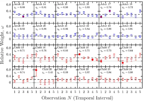
B. Results 422
We begin by considering the data for each individual listener, shown in Figure 7. To the extent 423
that an overall pattern can be discerned, the general trend was towards response strategies that 424
prioritized the first (primacy) or last (recency) observation. However, there was considerable 425
individual variability in both response strategy and overall efficiency. Thus, while Adult 13 and 426
Child 14 both up-weighted the first/last observation, and down-weighted the central observation, 427
Adult 17 exhibited the inverse pattern: relying predominantly on the 3rd observation, and
428
relatively little on the first/last observations. Only one listener (Child 20) appeared to base their 429
responses on only a single observation. However, few listeners approximated the ideal -- though 430
even in this respect were exceptions (cf. Adult 19, Adult 24, Child 15). Individual variability in 431
weight efficiency, 𝜂𝜔, was positively correlated with response precision [Pearson’s linear
432
correlation: r22 = 0.58, p = 0.003] – with more efficient weightings associated with lower response
433
variability. This suggests that the reverse correlation method reliably captures performance-434
436
FIG 7. Experiment II:Relative weight vectors for all individuals, with bootstrapped 95% standard error bars. Dashed 437
lines show the ideal weight vector. Shaded markers denotate instances where empirical weights deviated 438
significantly from the ideal. Individual children have been ordered by age (ascending). 439
A significant difference in integration efficiency, 𝜂𝜔, was observed between children and adults
440
[t22 = 2.49, p = 0.021], with adults tending to exhibit more efficient decision strategies [Fig 8A]. To
441
confirm that this difference was not due to one poor performing child (see Fig 8A), this analysis 442
was also repeated with this individual excluded [t21 = 2.33, p = 0.030], and using a non-parametric
443
analog [Wilcoxon rank sum; Z = 2.17, r = 0.44, p = 0.030]. In both cases, the same age-difference
444
was found.Both children [t11 = -6.50, p < 0.001] and adults [t11 = -8.29, p < 0.001] differed
445
significantly from the ideal observer [horizontal dashed line] – indicating that, on average, both 446
age-groups were suboptimal. 447
To examine the developmental time-course, Figure 8B plots integration efficiency as a function of 448
age. Based on the best fitting broken-stick function, it appears that adult-like performance was 449
limits of the adults (Fig 8B, shaded region). Furthermore, the fitted curve only explained 44% of 451
the variability in the raw data (R2 = 0.44), and the range of values between individual adults (𝜂
𝜔:
452
0.73 - 0.92) was greater than the model-difference between children and adults (Minima/Maxima 453
of fitted curve: 0.70 -- 0.84). Taken together, these results indicate that auditory integration does 454
not mature until around 11 years, but that the developmental effect in late childhood is small, 455
relative to the amount of individual variability between listeners. 456
[image:26.595.212.387.256.631.2]457
FIG 8. Experiment II:Integration efficiency for children and adults. (A) Group-mean [± 1 S.E.] integration efficiency 458
(same data as Fig 6). Markers indicate values of 𝜂𝜔 for individual subjects (one outlier at {10.2, 0.45} was excluded 459
from analysis, but is shown here for completeness). Horizontal dashed line represents the ideal observer. (B)
460
Integration efficiency as a function of age. The solid line represents the best-fitting piecewise polynomial (‘broken-461
stick’) curve, in which the point inflection (dashed vertical line) was a free parameter. The grey shaded region 462
C. Interim Discussion 464
As per Experiment I, the results of Experiment II confirmed that children are able to integrate 465
successive observations of an auditory location cue in order to perform a perceptual averaging 466
task, but that neither children nor adults are, on average, ideal. Unlike Experiment I, however, a 467
significant difference was observed between children and adults, with younger children tending 468
to be less capable integrators than adults -- only reaching adult-like performance by 469
approximately 11 years of age. 470
This qualitative difference between experiments can be most parsimoniously attributed to the 471
use of a more accurate methodology in Experiment II. Thus, as discussed after Experiment I, it is 472
likely that at least some internal noise is irreducible, and will remain present even as N tends
473
towards infinity. The explicit addition of reducible external noise is expected to have swamped 474
any residual effects of irreducible internal noise, thereby providing a more accurate measure of 475
efficiency in Experiment II. 476
Experiment II further allowed us to study why and in what way individual listeners were 477
suboptimal. Typically, the pattern was towards primacy and/or recency, with listeners giving too 478
great an importance to the first/last observation. There was, however, considerable individual 479
variability, with many listeners exhibiting their own individual listening strategies. 480
The tendency of some listeners to overweight the first observation is reminiscent of the 481
Precedence Effect, whereby multiple sounds presented in quick succession are heard as a single 482
“fused” image whose perceived direction is skewed towards the location of the first-arriving 483
sound (for a review, see Reference [30]). This is a primarily low-level, sensory phenomenon that
484
ensures perceptual robustness by effectively filtering-out acoustic reflections in reverberant 485
environments, and is subserved primarily by peripheral adaptation and inhibition in the 486
main reasons. First, the stimulus properties are mismatched. Thus, convergent data from human 488
psychophysics and animal physiology indicate that localization dominance occurs for lead-lag 489
delays only up to approximately 10 ms30. This is an order of magnitude less than the 100 ms ISI
490
used in the present study. And while the temporal window of the Precedence Effect has been 491
found to increase to around 15—30 ms when stimuli are presented repeatedly31,32 (“buildup”) ---
492
or up to 50 ms when speech stimuli are used33, these values still remain well-below the current
493
ISI of 100 ms. Second, no detectable perception of fusion or echo was observed subjectively 494
during piloting. Third, the development time-course is mismatched. For simple stimuli the 495
Precedence Effect is believed to be adultlike by around 5 years34,35. It therefore seems unable to
496
explain the differences observed between older (8-14-year-old) children and adults in the 497
present study. Forth and finally, the Precedence Effect primarily biases perceived direction 498
towards the first sound (though limited up-weighting of the final sound has also been reported in 499
some listeners36–38). It therefore cannot explain the substantial individual variability in weight
500
profiles observed in the present study (see Figure 7). In short, while we cannot rule out its 501
influence completely, the Precedence Effect seems unlikely to be a significant factor in 502
understanding the present data. Instead the individual and developmental differences observed 503
appear more likely due to higher-order, cognitive factors relating to perceptual decision-making 504
(see General Discussion). 505
Notably, however, the Precedence Effect is itself not an entirely a low-level phenomenon, and can 506
also be affected by various cognitive factors, including the listener’s expectations (see Reference 507
[39]). Some relationship with the present findings therefore cannot be ruled out altogether, and it
508
remains an empirical question whether there is any correlation between performance on the 509
IV. GENERAL DISCUSSION
511
The aim of this study was to quantify how integration efficiency develops during childhood. Using 512
a multiple-observation, absolute-localization task it was shown that adults and older children are 513
capable of integrating auditory information across sequential observations. However, the 514
efficiency of both groups fell well below that of the ideal observer. Using Reverse Correlation, this 515
inefficiency was shown to manifest differently across individuals, although there was a general 516
tendency towards primacy/recency listening profiles. In terms of development, children were 517
found to be significantly less efficient than adults, and only reached adult-like efficiency by 518
around 11.4 years. However, the amount of development was relatively small compared to 519
individual variability between adult listeners. Taken as a whole, the data indicates that perceptual 520
averaging undergoes a protracted, but relatively gradual period of development during older 521
childhood. 522
A. Integration efficiency in children 523
Among studies of audition, the present data are most comparable to those of Leibold and Bonino 524
(2009)15. There, it was found that children’s detection thresholds for a pure signal in noise
525
improved progressively as the signal was repeated from 1 to 5 times. Furthermore, as in 526
Experiment I of the present study, the rate of improvement was similar among both children and 527
adults. These data provide converging evidence for the notion that children (in that study, as 528
young as five years) are capable of integrating sequential auditory observations. 529
Outside of audition, the idea that that children are less efficient integrators is consistent with an 530
extensive literature. For example, studies of multi-sensory integration have found young children 531
to overly fixate on individual cues on tests of navigation4, size/orientation discrimination5, and
532
stimulus detection6. While, in the general decision-making literature, young children have been
shown to be worse at combining purely conceptual constructs, such as probabilistic 534
information40,41, or risk-versus-reward42–44.
535
It has been suggested previously that the ability to integrate sensory information only reaches 536
maturations relatively late in a child's development8. In the present task, children’s behavior
537
became adult-like at approximately 11 years. This developmental time course is in good 538
agreement with studies of visual cue integration, where adult-like performance has been found to 539
emerge around 11-12 years9,10. However, the developmental effect in the present study was
540
modest. It was not detectable in Experiment I, and in Experiment II the effect size was small 541
relative to overall individual variability, with several younger children (< 11 years) performing as 542
well as some adults. Thus, while the present data support the general notion that perceptual 543
decision making continues to develop all throughout childhood, the changes in older childhood 544
appear relatively small. 545
B. Integration efficiency in adults 546
The finding that adults integrate sequential information sub-optimally is consistent with several 547
recent studies in vision. For example, Juni & Maloney (2012)13 performed a visual analog of
548
Experiment II. Adult observers made seven, sequential observations of a stochastic location cue 549
(with additive jitter noise), and likewise exhibited effective, but suboptimal integration. Also as in 550
the present study, considerable individual variability in weight vectors was observed. Thus, 551
recency effects were particularly noticeable in some listeners, while others favored early or 552
central intervals (see Figs A2 & A3 of Reference [13]). Similar findings for judgments of visual size,
553
position, and direction have also been reported14.
554
Within audition, the data from adults are also consistent with a number of previous works; in 555
particular, a study by Swets and colleagues12 in which listeners were asked to detect a tone
556
integration, but at a rate that was highly variable between individuals, and which generally fell 558
markedly below that of the ideal observer45. Furthermore, as in the present study, integration
559
efficiency improved markedly when external noise was added independently to each observation. 560
This is consistent with the notion that some internal noise is non-reducible, and that this 561
component is great enough limit the benefits of integration under noiseless listening conditions. 562
More generally, adult performance is also consistent with a number of other ‘multiple-563
observation’ tasks such as profile analysis26,46 and sample discrimination47 in audition, or
564
motion-averaging, in vision48, wherein it is often observed that listeners use only a fraction of the
565
information available, and exhibit substantial individual variability in terms of which – and how 566
many – channels they attend to. 567
C. Potential causes of inefficiency 568
Why did many individuals, and younger children in particular, fail to integrate information 569
efficiently? 570
One possibility is that the observed deficits are primarily perceptual, and that information is 571
being lost at the point of encoding due to interference --- either neural or acoustic --- between 572
each sensory observation. In favor of this is the fact that children are also known to exhibit 573
elevated levels of backwards-masking, and that, as in the present work, this deficit declines to 574
near adult-levels by around 11 years49. Against this, however, stands the fact that sounds in the
575
present study were separated by relatively long inter-stimulus intervals (100 ms): by which point 576
any effects of non-simultaneous-masking are generally long-since abolished50,51 (see also the
577
discussion regarding the Precedence Effect in Experiment II). Furthermore, it is difficult to see 578
how perceptual interference could explain the level of individual variability in weight-vectors 579
observed in Experiment II. Nor can it explain why the inefficiencies observed in adults are 580
attractive in its simplicity, it appears inconsistent with the nature of the stimuli and the pattern of 582
data observed. This ‘perceptual interference’ hypothesis could be tested empirically by increasing 583
the temporal interval or acoustic dissimilarity between observations, in which case the relative 584
inefficiency of younger children should be diminished. 585
A second possibility is that inefficiencies observed in some listeners fundamentally represent 586
limited processing capacity. Thus, a rational strategy for a system with limited memory or 587
attention would be to fixate on a subset of the available information channels. Working memory 588
in particular may be a limiting factor in the present study, due to the long stimulus sequence and 589
slow presentation rate. Thus, information may have been lost over the course of the trial either 590
due to memory decay (though cf. Fig 6B) and/or interference between the memory of each 591
observation (see Reference [52]). Consistent with this, several listeners up-weighted the first/last
592
observation: a common strategy in memory-limited tasks. Furthermore, the developmental time-593
course in the present study is also broadly consistent with reports that working memory 594
continues to improves up until the age of at least 11 years old53,54. This ‘working memory’
595
hypothesis predicts a correlation between efficiency in the present task, and measures of 596
auditory working memory55. It also predicts that children’s efficiency would progressively
597
decrease if the memory component of the task was made more demanding (i.e., by increasing the 598
N observations, or adding a second ‘dual’ task). Alternatively, if the number of cues were reduced,
599
then the relative difference between children and adults should be diminished. 600
The idea that performance is primarily memory-limited appears plausible. However, it would be 601
premature to assume that children’s poorer performance necessarily reflects a lack of capacity. 602
Consider, for example, a recent study in which children aged 6 to 11 years were asked to ‘find the 603
middle’ of N simultaneously presented visual stimuli (dots). There, it was observed that children
604
of the available stimuli (i.e., due to a lack of capacity). Notably though, as the number of stimuli 606
increased from 5 to 15, children actually became faster and more adult like in their responses. On 607
close inspection, this change in performance appeared to be related to shift in response strategy. 608
With small numbers of stimuli (< 6), children’s trial-by-trial responses were best predicted by a 609
strategy of ‘finding the smallest shape that enclosed the visible dots, and pointing to its center’ 610
rather than the ideal strategy of computing the arithmetic mean of the individual points. The 611
precise reason for this difference in response strategy is unknown. However, what those data 612
demonstrate is that poor performance does not necessarily imply the inability to implement an 613
ideal strategy efficiently. Instead, children in the present task may be opting to interpret the task 614
in a qualitatively different way to adults (i.e., and may even be implementing a different strategy 615
in an optimal manner). Such differences in task interpretation are difficult to evidence. However, 616
it could be achieved, in general terms, by formulating an alternative response model that predicts 617
an individual’s trial-by-trial responses more reliably than the vector-weighted sum of the 618
individual observations. 619
Fourth, a related class of explanation is that children may simply be slower to learn what the task-620
relevant information is, or how to weight each channel appropriately. In this respect, it is 621
interesting to compare the present task, which requires multiple channels of useful information 622
to be combined, with tasks of the inverse form, in which channels containing signal and noise 623
must be segregated. For instance, studies by Kopco and colleagues have found that lateralization 624
judgments in adults can, depending on the stimulus parameters, be biased towards or away from 625
a preceding distractor presented at a fixed location56,57. Similar, but even greater effects have also
626
been reported in children, where, unlike in adults56,57, distractor-induced bias have been
627
observed even when the perceptual similarity between target and distractor is substantial58.
628
Taken together with the present study, the fact that children appear to struggle both with over-629
information (in the present study), would seem to point towards a more generalized deficit in 631
children’s ability to identify and/or attend to task relevant information. Such considerations also 632
bring to mind Informational Masking (masking by energetically weak but unpredictable 633
distractors), which is also elevated in young children59, and which has likewise been attributed to
634
an over-integration of information (this time across frequency rather than space; i.e., a broad 635
‘attentional filter’59,60). Notably, the ability to listen selectively on Informational Masking tasks
636
has been found to improve with practice in adults61–63. This suggests that even for individual
637
adults, performance on the present multiple-observation task may be limited by their ability to 638
learn the task statistics. Furthermore, it may be that younger children are simply slower, on 639
average, to learn the extent to which each channel contains task-relevant information. This ‘slow 640
learning’ hypothesis predicts that the developmental effect would be reduced given sufficient 641
practice, or may increase if the task-statistics were made more complex (i.e., adding different 642
levels of external noise to each observation interval13,29).
643
Fifth and finally, it may be that some listeners voluntarily chose not to integrate across all of the 644
available observations. This might have happened if, for example, a listener came to suspect that 645
some observation intervals were unreliable, or that not all observations originated from the same 646
source location. Efforts were taken to ensure that the latter did not occur (see Experiment II 647
Methods), and anecdotally no such suspicions were reported. It is also not immediately apparent 648
why this would produce less integration in young children, nor why it would lead to the various 649
patterns of weights observed in Figure 7. For instance, the most parsimonious strategy if one 650
believed that the sounds were independent, would be to respond based on only a single 651
observation. Such a strategy was only observed in one listener: Child 20. (NB: Alternating reliance 652
on different individual observations could potentially have produced the more uniform weights 653
observed in other listeners, but is inconsistent with the observed correlation between weight-654
suboptimal integration observed Experiment I, where all observations were in fact located 656
identically (although, due to internal noise, even identical stimuli are sometimes liable to be 657
perceived as different64). Nonetheless, the possibility that some listeners chose to discount
658
certain observations cannot be ruled out. This possibility could be investigated experimentally by 659
systematically increasing the amount of external noise (i.e., the sigma parameter of the jitter 660
distribution). In this case one would predict to see discontinuities, with a rapid reduction in 661
weight-efficiency at the point where listeners started to notice discrepancies. 662
Listeners might also have decided to voluntarily ignore some channels for the sake of ease, 663
assuming that the integration of each additional observation incurs some non-trivial ‘cost’ in 664
terms of listening effort. Such differences in motivation are always a concern in developmental 665
studies, and pains were taken to ensure that children remained engaged and focused throughout 666
the experiment. Furthermore, from a developmental perspective, the fact that the one child (Child 667
20) who exhibited a relatively simple ‘single observation’ strategy was such a marked outlier in 668
terms of efficiency is encouraging, as it suggests that younger children were not simply the ‘tail 669
end’ of some normal distribution of motivation (see Fig 8B). However, the possibility that 670
differences in motivation affected performance of some individuals cannot be ruled out. It could 671
be probed empirically by including a subset of ‘high value’ trials (i.e., with an association financial 672
incentive, or some child-friendly equivalent). If differences in motivation/effort do affect 673
performance, then the difference between children and adults, or between individual adults, 674
should be diminished on such trials. 675
D. Absolute sound localization performance in children and adults 676
Although the present study was concerned primarily with integration efficiency, it may also be of 677
interest to consider how listeners’ sound-localization performance compared with data reported 678
For adults, the present data are most comparable to the ‘noise’ condition of Recanzone, 680
Makhamra, & Guard (1998)65, who measured absolute-localization performance using 200 ms
681
white noise bursts. Within the central ±17° (i.e., the range of the present study), response errors 682
were relatively stable, with a standard deviation of approximately 5°. This is in good agreement 683
with the present data in Experiment 1, where the group-mean standard deviation (‘imprecision’) 684
was 4.81° for adults and 5.53 for children° (Figure 2, N = 1 condition). The present values are also
685
comparable to those of Yost and Zhong (2014)18, who asked listeners to localize 200 ms noise
686
bursts of variable bandwidth and central frequency. There, RMS error (which, for an unbiased 687
listener, is equivalent to the standard deviation of errors) was approximately 7.5° for a 1 octave 688
bandpass noise centered on 2 kHz. This is somewhat higher than the value of 4.81° observed in 689
the present study. However, it also includes presentations of up to +75°, and localization ability is 690
known to decrease with eccentricity18. Conversely, at a single eccentricity of +15°, Yost and Zhong
691
reported a mean RMS error of approximately 4° for bandwidths between 1/6 to 2 octaves: a value 692
that is roughly consistent with the present value of 4.81° (measured with a bandwidth of 1 octave 693
only). 694
For children, we are aware of no directly comparable data. However, the finding that children’s 695
response precision in the N=1 condition was not significantly lower than adults is consistent with
696
a number of studies showing that Minimal Audible Angles are largely adult-like by 5 years34, and
697
that absolute localization performance is mature by around 6 years66,67 (for a review, see
698
Reference [3]). In short, in terms of absolute localization ability, the results of both children and
699
![FIG 1. Stimuli and test apparatus for both experiments. (A) The listener’s task was to locate the [single] source](https://thumb-us.123doks.com/thumbv2/123dok_us/1378216.91061/6.595.49.548.418.627/fig-stimuli-apparatus-experiments-listener-locate-single-source.webp)
![FIG 3. Experiment I: Group-mean [± 1 S.E.] response variability for children (red crosses) and adults (blue circles), shown as a function of N Observations](https://thumb-us.123doks.com/thumbv2/123dok_us/1378216.91061/15.595.50.251.99.311/experiment-response-variability-children-crosses-circles-function-observations.webp)
![FIG 5. Experiment I: Group-mean [± 1 S.E.] integration efficiency for children and adults (same data as Fig 4)](https://thumb-us.123doks.com/thumbv2/123dok_us/1378216.91061/16.595.52.519.94.424/fig-experiment-group-mean-integration-efficiency-children-adults.webp)
![FIG 8. Experiment II: Integration efficiency for children and adults. (A) Group-mean [± 1 S.E.] integration efficiency (same data as Fig 6)](https://thumb-us.123doks.com/thumbv2/123dok_us/1378216.91061/26.595.212.387.256.631/experiment-integration-efficiency-children-adults-group-integration-efficiency.webp)