City, University of London Institutional Repository
Citation
:
Bignozzi, V. & Tsanakas, A. (2016). Parameter uncertainty and residual estimation risk. Journal of Risk and Insurance, 83(4), pp. 949-978. doi: 10.1111/jori.12075This is the accepted version of the paper.
This version of the publication may differ from the final published
version.
Permanent repository link:
http://openaccess.city.ac.uk/14722/Link to published version
:
http://dx.doi.org/10.1111/jori.12075Copyright and reuse:
City Research Online aims to make research
outputs of City, University of London available to a wider audience.
Copyright and Moral Rights remain with the author(s) and/or copyright
holders. URLs from City Research Online may be freely distributed and
linked to.
City Research Online: http://openaccess.city.ac.uk/ [email protected]
Parameter uncertainty and residual estimation risk
∗
Valeria Bignozzi
†Andreas Tsanakas
‡September 29, 2014
Abstract
The notion of residual estimation risk is introduced in order to study the impact
of parameter uncertainty on capital adequacy, for a given risk measure and capital
estimation procedure. Residual estimation risk is derived by applying the risk
mea-sure on a portfolio consisting of a random loss and a capital estimator, reflecting the
randomness inherent in the data. Residual risk thus equals the additional amount
of capital that needs to be added to the portfolio to make it acceptable. We propose
modified capital estimation procedures, based on parametric bootstrapping and on
predictive distributions, which tend to increase capital requirements, by
compen-sating for parameter uncertainty and leading to a residual risk close to zero. In
the particular case of location-scale families of distributions, the analysis simplifies
substantially and a capital estimator can always be found that leads to a residual
risk of exactly zero.
Keywords: Parameter uncertainty, model uncertainty, bootstrap, predictive distribution,
location-scale families, risk measures, solvency.
∗This is a preprint of an article accepted for publication in theJournal of Risk and Insurance, c2004 the American Risk and Insurance Association.
†School of Economics and Management, University of Firenze, Italy; email:
‡Cass Business School, City University London; email: [email protected]
1
Introduction
Insurance decisions, such as pricing, reserving and capital setting, are informed by the
outputs of statistical risk models. Such models are typically parametric. However, the
true values of parameters are in principle unknown and must be estimated from samples of
relevant observations. Such samples are often very small and statistical error means that
the estimated parameter values can diverge substantially from the true values. The
poten-tial for error in estimated parameters, termed parameter uncertainty, introduces possible error into insurance decisions based on model outputs. For example, if the estimated
fre-quency used to model claims from a natural hazard is lower than the true one, insurance
policies may be under-priced and a portfolio of such policies under-capitalized. It is
con-ventional to view parameter uncertainty in the context of an otherwise correctly specified
risk model. If the model is not known with certainty, we talk of model uncertainty. Decisions sensitive to tails of distributions, for which limited information resides in
available data, are more sensitive to parameter error. Thus, there is particular focus on
applications where the extremes of loss distributions are of interest, for example when
setting capital by a tail risk measure like Value-at-Risk (VaR) and Tail-Value-at-Risk
(TVaR), or when pricing high reinsurance layers. Investigations by insurance practitioners
have shown that the impact of parameter uncertainty in realistic modeling applications
can indeed be very substantial, see Mata (2000) and Borowicz and Norman (2008). High
sensitivity to parameter error has also been demonstrated in the context of credit risk
modeling by McNeil et al. (2005) and in a banking context by Jorion (1996), who argues
that confidence bands should be reported alongside estimated VaRs. Cont et al. (2010)
study risk measurement procedures and their sensitivity to changes in data used for
estimation, with reference to the notion of qualitative robustness.
In an early response to parameter uncertainty, Venezian (1983) recommends an explicit
increase to insurer capital, with the adjustment reflecting estimation volatility. Allowance
for parameter uncertainty is now often made in actuarial risk models, see Cairns et al.
(2006) on stochastic mortality and longevity bond pricing and Verrall and England (2006)
on stochastic claims reserving. A broadly applicable response to parameter uncertainty
is to work with predictive distributions, arising as weighted averages of distributions with
different parameter values. Cairns (2000) argues in favor of a fully Bayesian approach to
capture parameter (as well as model) uncertainty. Predictive distributions tend to be more
volatile than distributions that are derived via point estimates of parameters and thus can
lead to more conservative decisions, see also Landsman and Tsanakas (2012). Gerrard
and Tsanakas (2011) show that the increase in VaR that using a predictive distribution
implies, is appropriate for restoring a frequentist failure probability to its required nominal
level.
In the present contribution we also study risk measurement procedures, but from a
perspective that is complementary to that of Cont et al. (2010). We introduce a criterion
for assessing, in monetary units, the impact of parameter uncertainty on capital adequacy.
We assume that the required capital for an insurance company is calculated by applying
to a random loss variable a risk measure that is positive homogeneous, translation
in-variant, and law invariant. Commonly used risk measures, such as VaR or TVaR, satisfy
these properties. A random sample for the loss is available and the estimated capital
is a function of that sample; we call this function the capital estimator. To assess the effectiveness of a capital setting procedure, the risk measure is applied to the difference
between the loss (a random variable representing process variability) minus the capital
estimator (a random variable reflecting variability due to estimation). The result of this
calculation we call residual estimation risk. If the distribution of the loss is known, the residual risk is zero. In general, residual estimation risk is not equal to zero and can be
viewed as the (deterministic) amount of capital that needs to be added to the capital
estimator such that the total position becomes acceptable. When the sample size grows,
the capital estimator typically converges to the unknown required capital and the residual
estimation risk thus goes to zero.
procedure, even though our focus is on parametric models. In particular, model
uncer-tainty can also be assessed via residual estimation risk, if model selection is data driven
and thus reflected in the capital estimator (Bignozzi and Tsanakas, 2013). A strength
of the proposed approach is that it allows to consistently rank different estimation
pro-cedures. We show that monotonicity and subadditivity of the risk measure ensure that
capital estimators are appropriately ranked with respect to stochastic dominance and
con-vex stochastic order. Moreover, residual risk is expressed in monetary units and derived
with reference to a risk measure that explicitly represents preferences.
Apart from quantifying residual estimation risk, in the context of parametric models,
we discuss modifications to the capital setting procedure that reduce or even eliminate
residual risk. The first approach we discuss is a parametric bootstrap correction to the
capital estimator. Since the exact value of residual risk generally depends on unknown
parameters, we rely on a simple plug-in estimator of residual risk. Under mild conditions
it is shown that this corrected capital estimator leads to an improvement in residual
risk and its effectiveness is demonstrated by numerical examples, including the common
log-normal and Pareto models. In the second approach we propose, capital is set using
a predictive distribution derived by standard Bayesian arguments. The good predictive
performance of Bayesian methods under frequentist criteria has been highlighted in the
literature (Smith, 1999; Datta et al., 2000; Gerrard and Tsanakas, 2011). Once more,
numerical examples show that use of the predictive distribution nearly eliminates residual
estimation risk.
In the special case of location-scale models, such as the normal and Student t
distri-butions, several simplifications appear. It is shown that residual risk is independent of
the location parameter and proportional to the scale parameter. It follows that a simple
modification of the risk measure used to set capital can lead to a residual risk of exactly
zero. For example, if a TVaR measure at given confidence level is used to set capital,
this may be adjusted by using a different confidence level, depending on the size of the
repeated bootstrap corrections to the capital estimator can be performed without
increas-ing computational cost, as no nested simulations are needed. Finally, it is shown that for
location families and for scale families, the use of a predictive distribution respectively
eliminates residual estimation risk and a closely related functional.
Throughout the paper, we deal with models such as the Pareto and the log-normal,
which can give rise to distributions with infinite means, either by the values taken by
parameter estimators or by the mixture involved in deriving predictive distributions.
Infinite-mean models do not allow the evaluation of coherent risk measures such as TVaR
(Neˇslehov´a et al., 2006). For this reason, we often use in examples a truncated version of
TVaR, which we call Range-Value-at-Risk (RVaR). This risk measure, already considered
by Cont et al. (2010), considers a larger part of the tail than VaR, but is not coherent
and is well defined even when the mean of the loss distribution is infinite.
In Section 2 we introduce the notion of residual estimation risk and present numerical
examples of its quantification. Section 3 discusses methods for controlling residual risk
applicable to general loss distributions, while Section 4 deals with the specific case of
location-scale families. Brief conclusions are given in Section 5. Details of calculations
are documented in the Appendix of Section 6.
2
Residual estimation risk
2.1
Risk measures
The financial loss of a portfolio is modeled by a random variableY, defined on a standard
non-atomic probability space (Ω,F,P). Thus, in the event{Y >0}a portfolio loss occurs,
while {Y ≤ 0} corresponds to a gain. The distribution of Y is F. When considering
parametric models, we write F ≡ F(·;θ) where θ ∈ Θ is a vector of parameters. All
inequalities between random variables are meant to hold P-a.s.
ρ(Y). (Whenever this notation is used, we implicitly assume that the distribution ofY is
such that ρ(Y) is well defined.) ρ(Y) is expressed in monetary units and may represent
a regulatory capital requirement, which is the interpretation we follow here. Following
Artzner et al. (1999), a loss is acceptable if ρ(Y)≤0 andnot acceptable if ρ(Y)>0. We consider in this paper only risk measures that satisfy the following four standard
properties, which are assumed throughout the paper and not explicitly stated further on.
Monotonicity: If Y1 ≤Y2, ρ(Y1)≤ρ(Y2).
Translation invariance: If a∈R, ρ(Y +a) =ρ(Y) +a;
Positive homogeneity: If λ≥0, ρ(λY) =λρ(Y);
Law invariance: If Y1
d
=Y2, ρ(Y1) =ρ(Y2),
where = denotes equality in distribution.d
Law invariance requires that two losses with the same distribution have the same
capital requirement. Because of this, a risk measure can also be evaluated as a functional
of a distribution, such that for Y ∼F we may denote ρ(Y)≡ρ[F]. With this notation,
translation invariance and positive homogeneity can be written as ρ[F(· −a)] =ρ[F] +a
and ρ[F(λ·)] =λρ[F] respectively.
Three risk measures satisfying the above properties are
VaRp(Y) := inf{a∈R | P(Y ≤a)≥p}=F−1(p), (1)
TVaRp(Y) :=
1 1−p
Z 1
p
VaRu(Y)du=E(Y|Y > F−1(p)), (2)
RVaRp1,p2(Y) :=
1
p2−p1
Z p2
p1
VaRu(Y)du=E(Y|F−1(p1)< Y < F−1(p2)). (3)
The second equality in each of (1), (2), and (3), holds under the additional assumption
that the distributionF is invertible. All three risk measures are special cases of the general
class ofdistortion risk measures (Wang et al., 1997). The VaRp measure, used extensively
in insurance and banking regulation, is the 100pthpercentile of the loss distribution. VaR p
and Blake (2006). TVaRp corrects for this defect by considering the average of all VaRs
above the 100pth percentile. However, this introduces sensitivity to extreme percentiles,
which may not be reliably estimable from limited data. Furthermore, TVaR is not defined
for distributions with infinite means. RVaRp1,p2, proposed by Cont et al. (2010), offers a
compromise between those two risk measures: while it considers most of the tail, it does
not reflect some very extreme losses that a TVaRp1 measure would consider. Thus, for p2 <1 is always well defined.
An additional property often required is:
Subadditivity: For every Y1, Y2, ρ(Y1 +Y2)≤ρ(Y1) +ρ(Y2),
Risk measures satisfying monotonicity, translation invariance, positive homogeneity and
subadditivity are termed coherent, see Artzner et al. (1999). Of the three risk measures discussed above, only TVaR is subadditive and thus coherent.
2.2
Residual estimation risk
For the loss Y, the value of a law invariant risk measure depends on the distribution
function F, which is typically unknown and needs to be estimated from data. An i.i.d.
random sample of sizen from F will be denoted by X={X1, . . . , Xn}; with slight abuse
of notation we write X∼F. We assume that Y is independent of X. It follows that the
capital that the holder of Y needs to hold, with reference to the risk measureρ, will also
depend on the random sample itself and is denoted byη(X). Similar to Cont et al. (2010),
risk measurement is viewed as a two-step procedure. First the distribution F needs to
be estimated from data; denote the estimator of the distribution by FX. Second, the risk
measureρ is evaluated at FX, yielding the capital estimator η(X) =ρ[FX].
Cont et al. (2010) investigated the robustness of risk measurement procedures with
respect to small changes in the data set. They consider the notion ofqualitative robustness, which is closely related to weak continuity of statistical functionals. In this paper we offer
estimation volatility on capital adequacy, rather than robustness.
From translation invariance we have
ρ(Y −ρ(Y)) = 0, (4)
such that, by monotonicity, ρ(Y) is the minimal amount of capital that needs to be
subtracted from the lossY to make it acceptable. Reflecting the variability in the random
sampleX, we can considerY −η(X) as the random variable that represents the loss, after
the (random) capital estimator has been subtracted from it. We then define as residual estimation risk the quantity
RR(F, η) =ρ(Y −η(X)). (5)
Equation (5) is analogous to (4), with the theoretical capital value ρ(Y) substituted by
the capital estimator η(X). A positive residual risk implies that the impact of model
uncertainty is such that subtracting the capital estimator η(X) from the loss Y does not
produce an acceptable loss. Hence more safely invested capital needs to be held. The
residual estimation risk thus reflects the extra amount of capital that needs to be added
to the estimated capital η(X) in order to make Y acceptable, in particular it holds that
ρ(Y −(η(X) + RR(F, η))) = 0.By its definition, residual risk depends on the risk measure
ρ; this dependence is suppressed in the notation.
Of course, alternative measures of model and parameter uncertainty are available.
For example, confidence intervals for the estimated risk measure ρ[FX] can be calculated.
However, such an approach does not provide clear guidance about how risk estimates
should be plausibly adjusted, e.g. at which confidence level ofρ[FX] capital should be set.1
By measuring model risk in monetary units and associating it with the risk measure itself,
stated risk preferences provide guidance on designing capital setting procedures, as will be
seen in Section 3. Furthermore, the presence of the future lossY and a related estimator in
the same expression distinguish the present approach from uncertainty assessments based
1The issue of how risk measures should be calibrated, e.g. what the confidence level of VaR should be
on e.g. confidence intervals, by placing it in the broader context of predictive inference
(see e.g. Barndorff-Nielsen and Cox, 1996) and associating it with current considerations
of backtesting and model validation, see McNeil et al. (2005, Section 4.4.3) and Ziegel
(2014).
Before elaborating on that last point, some elementary properties of residual
estima-tion risk are collected. First, recall the definiestima-tions of stochastic dominance and convex
order for random variables (see Denuit et al., 2005, Sections 3.3-3.4). The random
vari-able S is smaller than T in stochastic dominance, S st T, if VaRp(S)≤VaRp(T) for all
p ∈ [0,1]. Intuitively S st T implies that S is a smaller risk than T; in particular one
can always find S0 =d S, T0 =d T such that P(S0 ≤ T0) = 1. The variability of S and T
can be compared via the convex order. S is smaller than T in convex order, S cx T, if
E(v(S))≤E(v(T)), for all convex functionsvsuch that the expectations exist. Immediate
consequences of S cxT are E(S) =E(T) and Var(S)≤Var(T).
Proposition 2.1. For a risk measure ρ and distribution F, the following hold:
a) For any distribution F∗, it is RR(F, ρ[F∗]) = ρ[F]−ρ[F∗].
b) If η1(X)st η2(X), then it is RR(F, η1)≥RR(F, η2).
c) If η(X)≥(≤)ρ[F], then it is RR(F, η)≤(≥)0.
d) If ρ is subadditive and satisfies the Fatou property, then η1(X) cx η2(X) implies
RR(F, η1)≤RR(F, η2)
e) If ρ is subadditive and η(X) = λη1(X) + (1−λ)η2(X) holds for all λ ∈[0,1], then
it is RR(F, η)≤λRR(F, η1) + (1−λ)RR(F, η2).
Proof. Part a) follows from translation invariance ofρ. For part b), by Proposition 3.3.17 in Denuit et al. (2005) it is Y −η2(X)st Y −η1(X). The stated inequality then follows
from monotonicity of ρand Theorem 4.1 of B¨auerle and M¨uller (2006). Part c) is similar
Proposition 3.4.25 in Denuit et al. (2005) it is Y −η1(X) cx Y −η2(X). The result
then follows from subadditivity and positive homogeneity of ρ (implying convexity) and
Theorem 4.2 of B¨auerle and M¨uller (2006). Part e) follows directly from subadditivity
and positive homogeneity of ρ.
Part a) of Proposition 2.2 implies that estimating capital using a fixed distribution
F∗ (essentially ignoring the data) leads to residual risk equal precisely to the difference
between the true and estimated level of capital, which is a simple measure of model
error. Part b) shows that choosing a larger capital estimator, in the sense of stochastic
dominance, will lead to a reduction in residual risk. Part c) is a special case of b):
designing a capital estimator that is always larger than the required capital under the
true distribution guarantees negative residual risk. Finally, part d) shows that residual
risk penalizes volatile capital estimators, for risk measures that are subadditive and satisfy
the Fatou property (a continuity requirement satisfied by all risk measures considered here
– see B¨auerle and M¨uller (2006) for details). Finally, the convexity of RR in η (part e) is
desirable as it implies that averaging of two capital estimators will lead to a residual risk
that is an improvement on the worst performing of the two.
The properties of residual estimation risk induce quality rankings of capital estimators.
This relates, but is distinct, to the discussion of elicitability of risk measures, which concerns the potential for assessing the quality of individual risk forecasts via a particular
scoring rule – see Gneiting (2011) and Ziegel (2014) for more detail. A full discussion of
elicitability is beyond the scope of this paper, but we note two key differences. First, in
our context the future loss is compared to an estimator (a random variable) rather than
a fixed forecast, allowing the assessment of the quality of risk measurement procedures
rather than individual forecasts. Second, the scoring approach penalizes all deviations
between forecasts and realized losses, while residual risk is allowed to be negative, thus
distinguishing between scenarios of potential under- and over-capitalization.
par-ticular case of ρ≡VaRp, η(X) = VaRp[FX]. Then, the equivalence holds,
RR(F, η) = VaRp(Y −η(X))≥0⇔P(Y > η(X))≥1−p. (6)
The right-hand-side of inequality (6) signifies a probability of failure (future loss exceeding
the capital estimator) higher than the acceptable level 1−pand was used as a measure of
parameter uncertainty by Gerrard and Tsanakas (2011). The quantity P(Y > η(X)) can
be interpreted as the expected relative frequency of violations when backtesting a VaR
model. Hence, the definition of residual estimation risk (5) can be related to a backtesting
criterion for risk measures more general than VaR; see the discussion on backtesting VaR
and TVaR in McNeil et al. (2005), Section 4.4.3.
2.3
Residual risk and parameter estimation
In the rest of the paper (with the exception of Example 11), we focus on residual risk due
to parameter rather than model uncertainty. Hence from now on we setF ≡F(·;θ), where
the distribution familyF(·;·) is known, but the parameterθneeds to be estimated.
Conse-quently, we simplify notation somewhat and write from now on RR(θ, η)≡RR(F(·;θ), η).
The residual risk depends on unknown but true parameters. This is similar to other
stan-dard frequentist quality criteria such as e.g. the mean-squared-error.
By ˆθ we denote an estimator of θ based on the random sample X. Unless
other-wise specified, parameters are estimated by likelihood maximization, such that η(X) =
ρ[F(·; ˆθ)] is the MLE of ρ[F(·;θ)].
We now present examples to illustrate the impact of parameter uncertainty on different
risk measures and distributions. In all numerical examples in this paper, the residual risk
ρ(Y − η(X)), for any distribution and capital estimator, is calculated numerically via
Monte-Carlo simulation. The precise details of the simulation algorithm are given in
Section 6.1. To allow comparisons, we will report in examples a normalized version of
residual risk:
NRR(F, η) = RR(F, η)
In all examples the denominator ρ(Y)−E(Y) is analytically calculated.
Example 1 (Normal, MLE). First consider a simple normal model, Y,X ∼ N(µ, σ2).
The mean µ and the standard deviation σ are unknown. Hence F(·; (µ, σ)) ≡ Φ ·−σµ
,
where Φ is the standard normal distribution. The standard normal density is denoted by
φ. We can write Y =d µ+σZ, where Z ∼ N(0,1). The MLE (ˆµ,σˆ2) satisfies (ˆµ, σˆ2)=d
µ+ √σ nU,
σ2V
n
,
where U ∼ N(0,1) and V ∼χ2n−1, withU, V independent.
By the translation invariance and positive homogeneity of ρit isρ(Y) = µ+σc, where
c=ρ(Z). The capital estimator becomes
η(X) = ρ[F(·; (ˆµ,σˆ))] =µ+√σ
nU +σ
r
V nc.
Consequently, the residual risk can be calculated as
RR((µ, σ), η) = σρ Z −√1 nU−
r
V nc
!
,
whereZ is independent ofU, V. The residual risk thus does not depend on the mean and
is proportional to the standard deviation. Furthermore, normalization as in (7) gives the
parameter free quantity, NRR((µ, σ), η) = ρ
Z−√1 nU−
√ V nc
c . In Section 4 it will be seen
that this is generally the case for location-scale families.
Table 1: Normalized residual estimation risk for a normally distributed risk with risk measure TVaRp, and the MLE capital estimator.
n=20 n=50 n=100 p=0.95 0.112 0.046 0.023 p=0.99 0.141 0.059 0.030 p=0.995 0.154 0.065 0.033
Table 1 presents the normalized residual risks for TVaRp and different values of pand
n. For this risk measure, it isc=TVaRq(Z) = φ(Φ
−1(q))
1−q (e.g. McNeil et al., 2005, Example
2.18). The values obtained demonstrate the substantial sensitivity of residual risk on the
of the required capital, while for a moderate sample of n = 100, the residual risk takes
values around 3% of capital.
For the commonly used log-normal model, some of the simplicity of Example 1 is lost.
Example 2 (Log-normal, MLE). Let Y0 ∼ N(µ, σ2) such that Y =eY0 is a log-normal
random variable. Here we use an RVaRp1,p2(Y) measure, which can be calculated as
RVaRp1,p2(Y) =
1
p2−p1
Z VaRp2(Y)
VaRp1(Y)
1
t√2πσ2te
−(ln(t)σ−µ)2
dt
= e
µ+12σ2 p2−p1
Φ(Φ−1(p2)−σ)−Φ(Φ−1(p1)−σ)
.
Thus the capital estimator is
η(X) = e
ˆ
µ+12σˆ2 p2−p1
Φ(Φ−1(p2)−σˆ)−Φ(Φ−1(p1)−σˆ)
.
The residual risk for a log-normal random variable is given by
RR((µ, σ), η) = RVaRp1,p2 Y −
eµˆ+12ˆσ2 p2−p1
Φ Φ−1(p2)−ˆσ
−Φ Φ−1(p1)−σˆ
!
,
where (ˆµ,σˆ2) is a random variable with the same distribution as in Example 1.
Values of normalized residual estimation risk for the log-normal distribution are
pre-sented in Table 2. For (µ, σ), the parameter choices (4.6002,0.0998) and (4.4936,0.4724)
are used, corresponding to the same mean E(Y) = 100 and coefficients of variation
CV(Y) = pVar(Y)/E(Y) taking values 0.1 and 0.5 respectively. A substantial
depen-dence of the normalized residual risk on the coefficient of variation is observed, with a
more volatile distribution leading to higher residual estimation risks. Residual risk is also
greater for higher p1, corresponding to risk measures focusing further in the tail.
Coherent risk measures, such as TVaR, are not well defined for random losses with
infinite means (e.g. Neˇslehov´a et al., 2006). The implication of this for the quantification
of residual risk are illustrated in the following example.
Example 3 (Pareto, MLE). Let Y,X follow a one-parameter Pareto with distribution
function F(y;θ) = 1−y−1/θ, y ≥1, which has a finite mean for θ <1. The MLE of θ is
ˆ
θ = n1 Pn
Table 2: Normalized residual estimation risk for a log-normally distributed risk with risk measure RVaRp1,0.997, and the MLE capital estimator.
CV(Y) = 0.1 CV(Y) = 0.5 n=20 n=50 n=100 n=20 n=50 n=100
p1 = 0.95 0.119 0.049 0.025 0.163 0.071 0.037
p1 = 0.99 0.147 0.062 0.031 0.200 0.091 0.048
p1 = 0.995 0.156 0.066 0.034 0.212 0.098 0.052
Table 3: Normalized residual estimation risk for a Pareto distributed risk, risk measure RVaRp1,0.997, and MLE capital estimator.
θ= 0.1 θ = 0.5
n=20 n=50 n=100 n=20 n=50 n=100
p1 = 0.95 0.130 0.057 0.030 0.207 0.107 0.060
p1 = 0.99 0.156 0.071 0.038 0.227 0.123 0.070
p1 = 0.995 0.165 0.077 0.040 0.237 0.130 0.075
parameters a and b. It is apparent that P(ˆθ ≥ 1) > 0. Hence even though E(Y) < ∞,
there are probable outcomes of ˆθ such that the capital estimator η(X) = ρ[F(·; ˆθ)] is not
well defined for coherent risk measures, such as TVaR, that require a finite mean. As a
consequence, the residual risk RR(θ, η) =ρ(Y −ρ[F(·; ˆθ)]) may also be not well defined.
For the Pareto distribution, simple computations lead to
η(X) = RVaRp1,p2[F(·; ˆθ)] =
1
p2−p1
1 ˆ
θ−1
(1−p2)1− ˆ
θ−(1−p
1)1− ˆ
θ.
The residual estimation risk becomes
RR(θ, η) = RVaRp1,p2
Y − 1
p2−p1
1 ˆ
θ−1
(1−p2)1− ˆ
θ−(1−p
1)1− ˆ
θ
,
where ˆθ∼Gam(n, θ/n) is once more considered as a random variable.
Normalized residual estimation risks for the Pareto distribution are presented in
Ta-ble 3 for parameter values θ = 0.1 and θ = 0.5 (corresponding to the case of an infinite
variance). The risk measure RVaRp1,p2 is used throughout, with p1 ∈ {0.95,0.99,0.995}
and p2 = 0.997. Consistently with Example 2, residual risk increases in θ (more heavy
3
Controlling residual estimation risk
A further step beyond quantification of residual risk is its control, that is, the design
of capital estimators that produce a residual risk (close to) zero. In all cases we have
considered, residual risk under an MLE capital estimator is positive. Consequently, the
capital estimation procedures we propose here tend to increase the capital in relation to
the MLE.
3.1
Parametric bootstrap
In this section, we aim to adjust η(X) via estimation of the residual risk RR(θ, η) that it
gives rise to. Since RR(θ, η) specifically depends on the unknown parameter θ, it is not
known to an agent who just observes the random sample X. Thus RR(θ, η) needs itself
to be estimated from the data.
This approach is a form of parametric bootstrapping; the overall principle is as follows.
Let the distribution of the parameter estimator ˆθ be G(·;θ). Then, given ˆθ, the
boot-strapped estimator ˆθ∗ is defined as having distribution G(·; ˆθ). The relationship between
ˆ
θ∗ and ˆθ mirrors the relationship between ˆθ and θ, which is required for inference. For a
rigorous treatment of the bootstrap see Hall (1992).
To make these notions more explicit, first denote by r1(θ) = RR(θ, η) the residual
estimation risk as a function of only the true parameter θ. As before, η(X) = ρ[F(·; ˆθ)],
where ˆθ is the MLE ofθ. Since we can interpretr1(θ) as the additional capital that needs
to be subtracted fromY −η(X) in order to make it acceptable, it is reasonable to propose
the followingfirst order bootstrap capital estimator
ηbs1(X) = η(X) +r1(ˆθ) = ρ[F(·; ˆθ)] +r1(ˆθ). (8)
In order to calculate r1(ˆθ) = RR(ˆθ, η), for a given realization of ˆθ, it is necessary to
simulate from the random variable ˆθ∗|θˆ∼G(·; ˆθ). The details of this simulation are given
in Section 6.2.
estimator. Let the residual risk arising from using the capital estimator ηbs1 be r2(θ) =
RR(θ, ηbs1). Consequently, we can define the second order bootstrap capital estimator as
ηbs2(X) =ηbs1(X) +r2(ˆθ) = ρ[F(·; ˆθ)] +r1(ˆθ) +r2(ˆθ), (9)
and the associated residual risk by r3(θ) = RR(θ, ηbs2). The process can be further
re-peated in order to derive bootstrap capital estimators of higher orders.
Proposition 3.1 shows that under weak conditions repeated applications of the
boot-strap correction generally produce an improvement in residual risk. In particular,
mono-tonicity of the risk measureρensures that the bootstrap correction operates in the correct
direction. Subadditivity of ρ, combined with a weak requirement on the volatility of the
estimator of residual risk, ensures the correction does not over- or under-shoot. The
proposition is formulated in relation to a bootstrap correction applied to a generic
cap-ital estimator η(X), which may itself be the product of a previously applied bootstrap
correction; we thus drop the subscript from the function r(θ).
Proposition 3.1. For X, Y ∼F(·;θ), parameter estimator θˆ, risk measureρ, and capital estimator η(X), define r(θ) = RR(F, η) and η∗(X) =η(X) +r(ˆθ).
a) If r(θ)≥0 for any θ∈Θ, then RR(θ, η∗)≤r(θ).
If in addition ρ is subadditive and ρ(r(ˆθ))≤2r(θ), then it is RR(θ, η∗)≥ −r(θ).
b) If r(θ)≤0 for any θ∈Θ, then RR(θ, η∗)≥r(θ).
If in additionρ is subadditive andρ(−r(ˆθ))≤ −2r(θ), then it isRR(θ, η∗)≤ −r(θ).
Proof. To prove part a), by monotonicity we have
RR(θ, η∗) = ρ(Y −(η(X) +r(ˆθ))) ≤ρ(Y −η(X)) =r(θ).
From the subadditivity ofρit follows thatρ(Y −(η(X) +r(ˆθ)))≥ρ(Y −η(X))−ρ(r(ˆθ)).
The assumptionρ(r(ˆθ))≤2r(θ) implies RR(θ, η∗) = ρ(Y −η(X))−ρ(r(ˆθ))≥ −r(θ).Part
b) follows similarly.
Here we demonstrate the effectiveness of the bootstrap approach for the log-normal
Example 4 (Log-normal, bootstrap). Expressions of the MLE capital estimator η(X)
and the corresponding residual risk r1(µ, σ) = RR((µ, σ), η) are given in Example 2.
Consequently the bootstrap capital estimator isηbs1(X) = η(X) +r1(ˆµ,ˆσ),where for each
estimate (ˆµ,σˆ) it is
r1(ˆµ,σˆ) = RVaRp1,p2 Y
∗−eµˆ
∗+1 2ˆσ
∗2
p2−p1
Φ Φ−1(p2)−σˆ∗
−Φ Φ−1(p1)−σˆ∗
!
,
where, given (ˆµ,σˆ), Y∗ follows a log-normal distribution with parameters (ˆµ,σˆ2) and
(ˆµ∗,σˆ∗) =d µˆ+ √σˆ
nU
∗, σˆ2V∗
n
, with U∗ ∼ N(0,1) and V∗ ∼ χ2n−1 independent. See Section 6.2 for a general description of the algorithm for derivingηbs1 by simulation.
Normalized residual risk is reported in Table 4. A dramatic improvement is observed
in comparison to the unadjusted MLE capital estimator (Table 2), with even a single
[image:18.595.139.459.406.483.2]application of the bootstrap correction leading to a residual risk of nearly zero.
Table 4: Normalized residual estimation risk for a log-normally distributed risk with risk measure RVaRp1,0.997, and first-order bootstrap corrected capital estimatorηbs1.
CV(Y) = 0.1 CV(Y) = 0.5 n=20 n=50 n=100 n=20 n=50 n=100
p1 = 0.95 0.001 -0.001 0.000 0.002 0.001 0.000
p1 = 0.99 0.001 0.000 0.000 0.002 0.001 0.000
p1 = 0.995 0.002 0.001 0.000 0.001 0.000 0.000
Table 5: Normalized residual estimation risk for a Pareto distributed risk, risk measure RVaRp1,0.997, and first-order bootstrap corrected capital estimator ηbs1.
θ= 0.1 θ = 0.5
n=20 n=50 n=100 n=20 n=50 n=100
p1 = 0.95 0.001 0.001 0.000 0.001 0.000 -0.002
p1 = 0.99 0.001 -0.002 -0.002 0.003 0.001 0.002
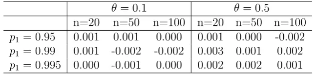
p1 = 0.995 0.000 -0.001 0.000 0.002 0.002 0.001
Example 5 (Pareto, bootstrap). Expressions of the MLE capital estimator η(X) and
[image:18.595.137.460.572.648.2]bootstrap capital estimator isηbs1(X) =η(X) +r1(ˆθ), where for each estimate ˆθ it is
r1(ˆθ) = RVaRp1,p2
Y∗− 1 p2 −p1
1 ˆ
θ∗−1
(1−p2)1− ˆ
θ∗
−(1−p1)1− ˆ
θ∗
,
where given ˆθ, Y∗ follows a Pareto distribution with parameter ˆθ and ˆθ∗ a Gamma
dis-tribution with parameters (n,θ/nˆ ).
Continuing from Example 3, residual estimation risk is calculated for a Pareto
distri-bution and the capital estimator ηbs1(X). Results are reported in Table 5. Once more,
residual risk is essentially eliminated, demonstrating a vast improvement in comparison
to the MLE capital estimator (Table 3).
3.2
Bayesian predictive distribution
The use of a Bayesian predictive distribution is a standard approach to dealing with
parameter uncertainty, see Cairns (2000). Under a Bayesian approach, the parameter
θ ∈ Θ is considered a random variable itself with prior distribution π(θ). Once data
x have been collected, the posterior of the parameter, π(θ|x), is obtained by π(θ|x) ∝ π(θ)Qn
i=1f(xi;θ). The predictive distribution of Y, given the data x, is defined as
ˆ
F(·|x) =
Z
θ∈Θ
F(·;θ)π(θ|x)dθ. (10)
Probabilities and expectations calculated according to the predictive distribution are
re-spectively denoted by ˆP(·|x) and ˆE(·|x).
Parameter uncertainty can be reflected in capital measurement by setting capital
ac-cording to the predictive distribution. That is, we set
ηbay(X) =ρ[ ˆF(·|X)]. (11)
Note the difference to the bootstrap capital estimators of Section 3.1: there an adjustment
to the MLE was produced, while here the probability distribution according to which
capital is set is modified.
Predictive distributions tend to be more dispersed in the tail, by their mixture
a reduction in the (typically positive) residual risk induced by an MLE capital estimator,
such that RR(θ, ρ[ ˆF(·|X)])≤RR(θ, ρ[F(·; ˆθ)]). While the residual risk is a frequentist
cri-terion, it has been widely noticed in the literature that Bayesian approaches to prediction
tend, at least approximately, to satisfy frequentist quality criteria (see Smith, 1999; Datta
et al., 2000). In fact, it follows from results of Gerrard and Tsanakas (2011) that, for a
wide set of loss distributions that includes the log-normal and Pareto examples discussed
here and the use of a non-informative prior, it is VaRp(Y −VaRp[ ˆF(·|X)]) = 0, such that
the residual risk is completely eliminated for VaR.
The effectiveness of the capital estimator ηbay is now demonstrated through examples.
It is seen the problems of infinite means emerge for both the log-normal and Pareto
models, motivating once more the use of RVaR.
Example 6 (Log-normal, Bayes). Let Y0,X0 ∼ N(µ, σ2) and Y = exp(Y0), X =
(exp(X10), . . . ,exp(Xn0)), such that Y,X ∼ LN(µ, σ2). For the log-normal distribution all moments exist, regardless of the value of the parameters, such that for a coherent risk
measure like TVaR, the quantity ρ[F(·; (ˆµ,ˆσ))] will always be well defined.
Consider now capital being set using the predictive distribution of Y, such that
ηbay(X) = ρ[ ˆF(·|X)]. A standard argument (similar to Hogg et al., 2012, Example 11.3.1)
shows that, using an uninformative prior π(µ, σ) = 1/σ, the predictive distribution of
the normal variable Y0 is a Student t distribution. Consequently, (see e.g. Gerrard and
Tsanakas, 2011, Lemma 1ii) the predictive distribution of the log-normal variable Y is a
“log-t” distribution
ˆ
F(y|X) =tn−1 r
n−1
n+ 1
log(y)−µˆ ˆ
σ
!
,
where ˆµ, σˆ are the MLEs of µ, σ, and tn−1 is the distribution function of a standard
Student t variable with n−1 degrees of freedom.
The expected value associated with ˆF(·|X) is ˆE(Y|X) = ˆE(exp(Y)|X). However,
since the Studentt distribution has a regularly varying tail (McNeil et al., 2005, p. 293),
its moment generating function is not well defined, implying that ˆE(exp(Y0)|X) = ∞.
estimator of the form ρ[ ˆF(·|X)] will also be infinite, when a coherent risk measure ρ is
used.
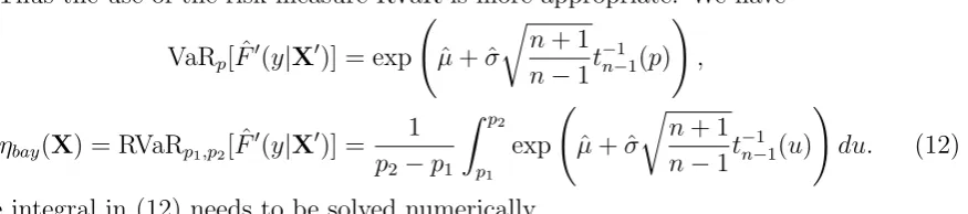
Thus the use of the risk measure RVaR is more appropriate. We have
VaRp[ ˆF0(y|X0)] = exp µˆ+ ˆσ
r
n+ 1
n−1t
−1
n−1(p) !
,
ηbay(X) = RVaRp1,p2[ ˆF 0
(y|X0)] = 1
p2−p1
Z p2
p1
exp µˆ+ ˆσ
r
n+ 1
n−1t
−1
n−1(u) !
du. (12)
The integral in (12) needs to be solved numerically.
The normalized residual estimation risk for the log-normal distribution is presented
in Table 6. It is seen that using the predictive distribution is highly effective in nearly
eliminating residual risk. In particular, comparison to Table 2 reveals the great
improve-ment achieved in relation to MLE, with residual risk for ηbay being close to zero. The
[image:21.595.91.529.128.225.2]performance ofηbay is thus comparable to that ofηbs1 reported in Table 4.
Table 6: Normalized residual estimation risk for a log-normally distributed risk, risk measure RVaRp1,0.997, and Bayes capital estimatorηbay.
CV(Y) = 0.1 CV(Y) = 0.5 n=20 n=50 n=100 n=20 n=50 n=100
p1 = 0.95 -0.005 -0.001 -0.001 -0.008 -0.003 -0.001
p1 = 0.99 -0.001 0.000 0.000 -0.001 0.000 0.000
[image:21.595.139.460.588.664.2]p1 = 0.995 0.000 0.000 0.000 0.000 0.000 0.000
Table 7: Normalized residual estimation risk for a Pareto distributed risk, risk measure RVaRp1,0.997, and Bayes capital estimator ηbay.
θ= 0.1 θ= 0.5
n=20 n=50 n=100 n=20 n=50 n=100
p1 = 0.95 -0.005 -0.002 -0.001 0.018 0.012 0.008
p1 = 0.99 0.000 0.000 0.000 0.007 0.006 0.004
p1 = 0.995 0.000 0.000 0.000 0.002 0.002 0.002
leads to a predictive distribution for Y of the form
ˆ
F(y|X) = 1− nθˆ
log (y) +nθˆ
!n
, (13)
where ˆθ is the MLE of θ. This is a “log-Pareto” distribution, again with infinite mean.
For the VaR and RVaR measures of Y we now have,
VaRp[ ˆF(y|X)] = exp
ˆ
θn((1−p)−1/n−1)
,
ηbay(X) = RVaRp1,p2[ ˆF(y|X)] =
1
p2−p1
Z p2
p1
exp
ˆ
θn((1−u)−1/n−1)
du. (14)
Again, the integral in (14) can be solved numerically.
The normalized residual estimation risk for the Pareto distribution is presented in
Table 7. Once more, the use of the predictive distribution is highly effective, leading
to residual risk levels very close to zero, thus improving on the MLE capital estimators
(Table 3).
4
Quantifying and controlling residual estimation risk
for location-scale families
In the current section we focus on residual estimation risk for distribution functions that
belong to location-scale families. Such distributions, like the normal, Student t, and
Laplace (double-exponential) families are commonly used in modeling asset returns. It
will be seen that the case of location-scale families allows substantial simplifications in
the quantification and control of residual risk. In particular, exact elimination of residual
risk is possible.
4.1
Residual estimation risk for location-scale families
Two random variables Y and Z belong to the same location-scale family, if there exist
Z ∼ F(·; (0,1)) has a standardized distribution and simply denote it by F ≡F(·; (0,1)).
Hence, we can write Y ∼F(·; (µ, σ)) = F ·−σµ
.
Estimators of location and scale parameters generally also belong to location-scale
families. Specifically, if the parameter vector θ = (µ, σ) is estimated via Maximum
Like-lihood, then a standard argument (e.g. Gerrard and Tsanakas, 2011, Lemma 4) shows
ˆ
µ=d µ+σU, σˆ=d σV, (15)
where U and V are random variables whose distribution depends on the sample size n,
but not on θ.
From the translation invariance, positive homogeneity, and law invariance properties
of the risk measure, it follows that for Y ∼F(·; (µ, σ)), Z ∼F, it is
ρ(Y) =ρ(µ+σZ) =µ+σρ[F].
Let the capital estimator be based on the MLE, such that η(X) = ρ[F(·; ˆθ)], where
ˆ
θ = (ˆµ,ˆσ). Thus, it is η(X) = ˆµ+ ˆσρ[F] =µ+σU +σV ρ[F].
Consequently, the residual estimation risk can be calculated as
RR(θ, η) =ρ(µ+σZ−µ−σU−σV ρ[F]) =σρ(Z −U−V ρ[F]). (16)
Hence, while in general the residual estimation risk remains unknown, for
location-scale families it does not depend on the location parameterµand is directly proportional
to the scale one σ. In particular, the amount ρ(Z −U −V ρ[F]) does not depend on the
unknown parameters. This effect was demonstrated in Example 1, when dealing with
normally distributed losses.
4.2
Adjustment to the risk measure
In the case of location-scale families it is possible to modify the risk measure in a way
that compensates for parameter uncertainty and brings the residual estimation risk down
risk measure, the capital estimator, using again MLE, will be
ηadj(X) =ρadj[F(·; ˆθ)].
Analogously with (16), we can write
RR(θ, ηadj) =ρ(Y −ρadj[F(·; ˆθ)]) = σρ(Z−U −V ρadj[F]). (17)
Noting that the quantityρ(Z−U−V ρadj[F]) does not depend on the true but unknown
parameterθ, it becomes apparent that we can choose the risk measureρadj[F] specifically
so as to set the residual risk of (17) to zero. For example, if ρ = TVaRp, we can let
ρadj = TVaRq for some q6=p. The process is illustrated by the following example.
Example 8 (Normal, adjusted TVaR). Consider a normal distribution and let ρ =
TVaRp, ρadj = TVaRq. The the random variables U, V in (15) become
U = √1 nU
0
, V =
r
V0
n ,
where U0 ∼ N(0,1) and V0 ∼ χn2−1, with U0, V0 independent. Noting that TVaRq(Z) = φ(Φ−1(q))
1−q , the residual risk under the adjusted capital estimator is
RR((µ, σ), ηadj) =σTVaRp Z −
1 √ nU 0 − r V0 n
φ(Φ−1(q))
1−q
!
,
and a level q that sets the above expression to zero can be found.
To simplify exposition, assume now that the scale parameter σ is known. Then
RR(µ, ηadj) =σTVaRp
Z− √1 nU
0− φ(Φ −1(q))
1−q
=σ
r
1 + 1
n
φ(Φ−1(p))
1−p −σ
φ(Φ−1(q))
1−q .
Therefore, to achieve RR(µ, ηadj) = 0, one needs to solve forq the equation
r
1 + 1
n
φ(Φ−1(p))
1−p =
φ(Φ−1(q))
1−q ,
which is easily done numerically. The resulting adjusted capital estimator thus is
ηadj(X) = ˆµ+σTVaRq(Z) = ˆµ+σ
r
1 + 1
nTVaRp(Z).
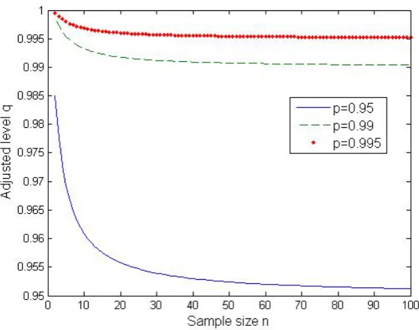
The required level of q is plotted in Figure 1, against the sample size n, for p ∈
Figure 1: Confidence levelqrequired to eliminate the residual estimation risk for a normal random variable with known scale parameter and risk measure TVaRp.
the adjusted confidence levelq decays to the nominal level p. The differenceq−pis more
pronounced for very small sample sizes, such that, if ηadj were adopted, portfolios with a
longer history would be subject to a lower capital requirement.
4.3
Bootstrap procedure for location-scale families
In Section 3.1 it was demonstrated that repeated bootstrap corrections to the capital
estimator produce improvements in residual risk. However, these improvements come
at a cost, since each iteration induces a nested simulation. Here it is shown that, for
location-scale families, higher order bootstrap capital estimators can be derived exactly,
avoiding the need for nested simulations.
the MLE and the first-order bootstrap capital estimator are
r1(θ) =σρ(Z−U −V ρ(Z)),
ηbs1(X) = ˆµ+ ˆσρ(Z) +r1(ˆθ) = µ+σU+σV(ρ(Z) +ρ(Z−U −V ρ(Z))). (18)
It follows that
r2(θ) = ρ(Y −ηbs1(X)) =σρ(Z −U−V(ρ(Z) +ρ(Z−U −V ρ(Z)))),
ηbs2(X) = ηbs1(X) +r2(ˆθ)
= ˆµ+ ˆσ[ρ(Z) +ρ(Z−U −V ρ(Z)) +ρ(Z −U −V(ρ(Z) +ρ(Z−U −V ρ(Z))))].
(19)
Since the distribution of the random variables Z, U, V does not depend on the true
pa-rameters (µ, σ), formulas (18) and (19) can be evaluated from a single set of simulated
values from Z, U, V. The above argument can be extended to an arbitrary number of
bootstrap iterations.
It is also noted that for the case of location families, where the scale parameter is
known, the first-order bootstrap corrected capital estimator gives an exact elimination of
residual risk. To see that, one may follow the same steps as above, setting without loss
[image:26.595.139.457.527.602.2]of generality V = 1. Then, r2(µ) = σρ(Z −U −(ρ(Z) +ρ(Z−U −ρ(Z)))) = 0.
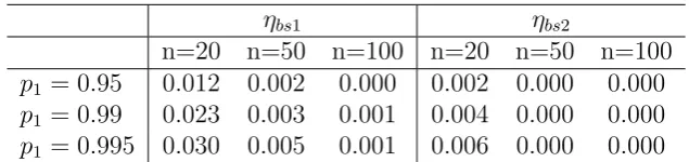
Table 8: Normalized residual estimation risk for a normally distributed risk with sample size n, risk measure TVaRp, and the bootstrap capital estimators ηbs1, ηbs2.
ηbs1 ηbs2
n=20 n=50 n=100 n=20 n=50 n=100
p1 = 0.95 0.012 0.002 0.000 0.002 0.000 0.000
p1 = 0.99 0.023 0.003 0.001 0.004 0.000 0.000
p1 = 0.995 0.030 0.005 0.001 0.006 0.000 0.000
Example 9 (Normal, bootstrap). Residual risk is now calculated for a normally
dis-tributed risk, a TVaRp risk measure, and the first- and second-order bootstrap capital
estimators ηbs1(X), ηbs2(X). Results are reported in Table 8. The first-order bootstrap
estimator, while the second-order bootstrap estimator reduces the capital even further.
In the particular case of a known standard deviation, we have
r1(µ) = TVaRp(µ+σZ−µˆ−σTVaRp(Z))
=σTVaRp
Z− √1 nU
0
−σTVaRp(Z)
=σ
r
1 + 1
nTVaRp(Z)−σTVaRp(Z), ηbs1(X) = ˆµ+σ
r
1 + 1
nTVaRp(Z).
Hence,ηbs1is exactly the same capital estimator asηadj considered in Example 8, satisfying
RR(µ, ηadj) = 0.
4.4
Bayesian predictive distribution for location-scale families
In this section we show that for location-scale families, (a) when the scale parameter is
known, residual risk is completely eliminated, and (b) when the location parameter is
known, a quantity similar to residual risk equals zero.
Before stating the results we reformulate without proof the content of Proposition 1 in
Severini et al. (2002), which is used in the present section. For the sake of simplicity, details
about the technical conditions are omitted, but Example 1 in Severini et al. (2002), implies
that location-scale families satisfy all the necessary conditions to apply the proposition.
Proposition 4.1. Severini et al. (2002). For Y,X∼F(·;θ)belonging to a location-scale family with θ = (µ, σ) ∈ Θ, let H(X) be a region such that Pˆ(Y ∈ H(X)|x) = 1−α.
Assume that H satisfies the following conditions:
(i) For each θ = (µ, σ) ∈ Θ, y ∈ H(x) if and only if y+µ ∈ H(µ+x) (for location models) and σy∈H(σx) (for scale models).
(ii) Let C(x, y) = 1 if y ∈ H(x) and 0 otherwise. There exists 0 < α < 1, such that
ˆ
E[C(X, Y)|x] = 1−α.
Consider first a location family with parameterθ =µ. The priorπ(θ) = 1 is used. It is
known that (e.g. see Gerrard and Tsanakas, 2011), if X=Z+b, where Z= (Z1, . . . , Zn)
and Z∼F, then ˆF(y|z+b) = ˆF(y−b|z). Therefore,
ρ[ ˆF(·|x)] = ρ[ ˆF(· −b|z)] =ρ[ ˆF(·|z)] +b,
due to the translation invariance property of ρ.
Proposition 4.2 shows that using the predictive distribution eliminates residual risk
for location families.
Proposition 4.2. For location families, using the capital estimator ηbay(X) =ρ[ ˆF(·|X)]
yields
ρ(Y −ηbay(X)) = 0.
Proof. The proof follows from an application of Prop. 4.1. Consider the predictive region
Hc(X) = (−∞, ρ[ ˆF(·|X)] +c]
for any constant c∈R. This region is invariant as required, indeed:
Y +b∈Hc(X+b)⇔Y +b ≤ ρ[ ˆF(·|X+b)] +c = ρ[ ˆF(·|X)] +b+c⇔
Y ≤ ρ[ ˆF(·|X)] +c⇔Y ∈Hc(X).
It follows that ˆP(Y −ρ[ ˆF(·|X)] ≤ c|x) = P(Y −ρ[ ˆF(·|X)] ≤ c) ∀c ∈ R. As this holds
for every c∈R, it is implied that the random variable W =Y −ρ[ ˆF(·|X)] has the same
distribution under ˆP(·|x) andP(·). Thus ifG(w) =P(W ≤w) and ˆG(w|x) = ˆP(W ≤w|x)
it is G(w) = ˆG(w|x) for all w. By law invariance of ρ it then is ρ[G(·)] = ρ[ ˆG(·|x)].
However, by the construction of the random variable W it is ρ[ ˆG(·|x)] = 0. Hence
ρ[G(·)] =ρ(Y −ρ[ ˆF(·|X)]) = 0.
Suppose now that Y belongs to a scale family, with parameter θ = σ. We use the
prior π(θ) = 1/θ. If X =bZ, where b >0, Z = (Z1, . . . , Zn) and Z ∼F, then ˆF(y|bz) =
ˆ
F(y/b|z). Therefore,
ρ[ ˆF(·|x)] =ρ[ ˆF(·/b|z)] =bρ[ ˆF(·|z)],
Proposition 4.3 shows that for scale-families the capital estimator ηbay(X) leads to
elimination of a scaled version of the residual risk.
Proposition 4.3. For scale families, using the capital estimator ηbay(X) = ρ[ ˆF(·|X)]
yields
ρ Y
ρ[ ˆF(·|X)] −1
!
= 0.
Proof. The same procedure as in the proof of Proposition 4.2 is followed. The predictive region is
Hc(X) = (−∞, cρ[ ˆF(·|X)]]
for any constant c∈R. This region is invariant as required in Prop 4.1, since
bY ∈Hc(bX)⇔bY ≤ cρˆ[ ˆF(·|bX)] = cbρˆ[ ˆF(·|X)]⇔
Y ≤ cρ[ ˆF(·|X)]⇔Y ∈Hc(X).
It follows that:
ˆ
P Y
ρ[ ˆF(·|X)] ≤c|x
!
=P Y
ρ[ ˆF(·|X)] ≤c
!
∀c∈R.
As this holds for everyc∈R, it is implied that the random variableW =Y /ρ[ ˆF(·|X)] has
the same distribution under ˆP(·|x) and P(·). Thus if G(w) = P(W ≤ w) and ˆG(w|x) =
ˆ
P(W ≤ w|x) it is G(w) = ˆG(w|x) for all w. By law invariance of ρ it then is ρ[G(·)] =
ρ[ ˆG(·|x)]. However, by the construction of the random variable W it is ρ[ ˆG(·|x)] = 1.
Hence ρ[G(·)] =ρ Y
ρ[ ˆF(·|X)]
= 1.
For the more general location-scale case, the effectiveness of using a predictive
distri-bution is demonstrated via the following example.
Example 10 (Normal, Bayes). For a normal distribution and prior π(µ, σ) = 1/σ, a
standard argument similar to Hogg et al. (2012, Example 11.3.1) shows that the predictive
distribution is a Student t distribution
ˆ
F(y|X) =tn−1 r
n−1
n+ 1
y−µˆ ˆ
σ
!
where ˆµ, σˆ are the MLEs of µ, σ, and tn−1 is the distribution function of a standard
t variable with n−1 degrees of freedom. The corresponding value of TVaR is (McNeil
et al., 2005, Example 2.19)
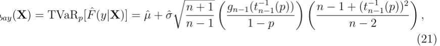
ηbay(X) = TVaRp[ ˆF(y|X)] = ˆµ+ ˆσ
r
n+ 1
n−1
gn−1(t−n−11(p))
1−p
n−1 + (t−n−11(p))2
n−2
,
(21)
where gn−1 is the density of a standard t variable with n−1 degrees of freedom. The
Studenttpredictive distribution is heavy-tailed, which generally leads to higher estimated
capital levels than the normal.
In Table 9 the corresponding normalized residual risks are reported. Once more, the
effectiveness of using ηbay is apparent, with a near elimination of residual risk observed.
The performance is comparable to the second-order bootstrap estimator seen in Table 8,
thoughηbay appears to slightly overcompensate in increasing capital estimates, leading to
[image:30.595.92.528.139.185.2]slightly negative residual risks.
Table 9: Normalized residual estimation risk for a normally distributed risk with sample size n, risk measure TVaRp, and the Bayes capital estimator ηbay.
n=20 n=50 n=100 p=0.95 -0.007 -0.003 -0.001 p=0.99 -0.005 -0.002 -0.001 p=0.995 -0.005 -0.002 -0.001
4.5
The presence of a shape parameter
There are location-scale families that have additional shape parameters, such as the
Student t distribution. For such distributions, the computational savings present for
location-scale families cannot be fully achieved, but their parametric structure can still
be exploited.
Consider a Student t random variable Y with parameters θ = (µ, σ, ν), such that
ˆ
θ = (ˆµ,σ,ˆ νˆ) be an estimator of θ. For many classes of estimators, such as MLEs and
the simple estimator described in Section 6.3, the random variables ˆµ,σˆ will still follow
a (location-)scale distribution, such that we may write, ˆµ=µ+σUν, σˆ =σVν, νˆ=Wν,
where the distribution of (Uν, Vν, Wν) does not depend on µ orσ but depends on ν.
For parameter estimator ˆθ, the unadjusted capital estimator is η(X) = ρ[F(·; ˆθ)] =
ˆ
µ+ ˆσρ[tνˆ], where tν is the distribution of a standard Student t variable withν degrees of
freedom. Consequently, the residual estimation risk can be written as
RR(θ, η) = ρ(µ+σZν −µˆ−σρˆ [tνˆ]) = σζ(ν),
where ζ(ν) =ρ(Zν −Uν −Vνρ[tνˆ]). (22)
Hence we can define the bootstrap estimator as
ηbs1(X) = ˆµ+ ˆσ(ρ[tˆν] +ζ(ˆν)). (23)
To implement this estimator, numerical evaluation of the function ζ(ν) is required. But,
as ζ does not depend on the distribution parameters, nested simulations are avoided.
These ideas are demonstrated via the following example, where the issue of model
error is also briefly discussed.
Example 11 (Student t, bootstrap, empirical, model error). In this example we work
with an RVaRp1,p2 risk measure, with p1 = 0.95, p2 = 0.997 and a Student t distribution
withθ = (µ, σ, ν) = (0,1,5), with all three parameters considered unknown in the capital
estimation. The RVaR measure of a standard t variable is given in Section 6.5). Sample
sizes n = 50,10,200,500,1000 are considered.
Subsequently we calculate the residual estimation risk for different capital estimators.
Details about how each of those capital estimators (and in particular the numerical
ap-proximation of ζ) simulated is given in Section 6.2; the assessment of residual risk for
each estimator is as described in Section 6.1.
Student t: This is an unadjusted estimator of RVaRp1,p2 obtained by estimating
Studentt (bootstrap): This is a bootstrap corrected estimator of RVaRp1,p2 obtained
asηbs1(X) = ˆµ+ ˆσ(RVaR[tνˆ] +ζ(ˆν)), with ζ(ν) as in (22).
Empirical: The RVaRp1,p2 measure is directly applied in a model-free way, by the
empirical distribution of the sample X.
Normal: The possibility of model error is considered, by assuming in capital es-timation that the data are actually from a normal distribution and applying the
[image:32.595.121.478.323.397.2]standard normal MLE of RVaR.
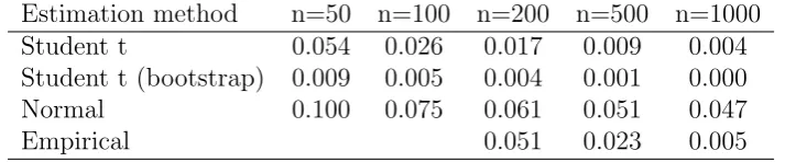
Table 10: Normalized residual estimation risk for a Studentt5 distributed risk with sample
size n, risk measure RVaR0.95,0.997, and various capital estimators.
Estimation method n=50 n=100 n=200 n=500 n=1000 Student t 0.054 0.026 0.017 0.009 0.004 Student t (bootstrap) 0.009 0.005 0.004 0.001 0.000 Normal 0.100 0.075 0.061 0.051 0.047
Empirical 0.051 0.023 0.005
The resulting residual estimation risk figures are shown in Table 10. For ηemp results
are only reported forn≥200, as estimation of the given RVaR measure is not meaningful
on smaller samples. The results demonstrate how the residual estimation risk of the
unadjusted estimator η is nearly eliminated by the bootstrap corrected estimator ηbs1.
The estimator ηnorm, accounting for the case of model error, presents a substantially
higher residual risk, due to the underestimation of required capital arising by the lighter
normal tail that it assumes. Furthermore, residual risk does not tend to zero for increasing
sample sizes. On the other hand, for n ≥ 200, the model-free empirical estimator ηemp
beats ηnorm, while at the same time performing worse than the estimators ηt, ηbst that
5
Conclusions
We introduce the notion of residual estimation risk for measuring the impact that the
volatility of risk estimators has on capital adequacy. Residual risk quantifies the capital
that needs to be added to a portfolio, consisting of a random loss and a random capital
estimator, in order to make the total position acceptable with reference to a risk measure.
In a parametric setting, this interpretation motivates the design of modified capital setting
procedures, based on bootstrapping and Bayesian predictive distributions. The good
performance of these approaches is demonstrated by numerical examples, both for general
distributions and for location-scale families, where exact elimination of residual risk is
always possible.
While our focus here is on parameter uncertainty, the idea of residual risk retains
its meaning in the broader context of model uncertainty. Under model uncertainty, it
is customary to consider a number of candidate models (families of distributions) for
the loss (Cairns, 2000; Kerkhof et al., 2010; Barrieu and Scandolo, 2013; Breuer and
Csisz´ar, 2014; Alexander and Sarabia, 2012; Boucher et al., 2014). Based on a random
sample, a suitable model may be chosen using either statistical criteria (e.g. goodness of
fit) or a worst-case scenario approach. Any such estimation procedure can be expressed
via a capital estimator as in this paper, such that the corresponding residual risk can be
quantified. An investigation of residual estimation risk in the context of model uncertainty
is performed by Bignozzi and Tsanakas (2013), where a disentangling of the distinct
impacts of parameter and model uncertainty is attempted.
Finally, we note that the proposed capital estimation procedures typically lead to an
increase in the calculated capital requirements, compared to e.g. MLE. However, this
does not mean that, if one of those procedures is followed, sufficient capital will certainly
be present for each individual portfolio. The proposed capital increases are designed
to be effective at an aggregate (e.g. market) level, with the outer risk measure in the
is thus implicit in our use of a frequentist statistical framework, where the volatility of
random samples may be best understood as variability in the experience of a group of
economic/statistical agents.
6
Appendix
6.1
Numerical evaluation of residual risk
Here we explain how the residual risk for different estimators is obtained via Monte-Carlo
simulation, using a simple importance sampling scheme. In all examples, we need to
calculate the quantity ρ(Y −η(X)), where ρ may be VaRp, TVaRp or RVaRp1,p2.
First m = 107 samples are simulated from the random variable η(X); denote these
as η1, . . . , ηm. (Details about simulation of η(X) are given in Section 6.2.)
Subse-quently, λmsimulated values, y1, . . . , yλm, are obtained from the conditional distribution
Y|Y > VaRu(Y) and (1−λ)m simulated values, yλm+1, . . . , ym, from Y|Y ≤ VaRu(Y).
Throughout, we use the values λ= 0.9 and u= 0.9. This ensures that a high fraction of
simulations is obtained for high values ofY leading to more frequent exceedances ofη(X)
byY. For each i= 1, . . . , msetzi =yi−ηi. Note that it is
P(Y −η(X)≤z) = (1−u)P(Y −η(X)≤z|Y >VaRu(Y))
+uP(Y −η(X)≤z|Y ≤VaRu(Y)). (24)
Hence we can approximate the distribution of Y −η(X) using the conditional empirical
distributions
P(Y −η(X)≤z)≈ 1−u
λm
λm
X
j=1
I{zj≤z}+ u
(1−λ)m
m
X
j=λm+1
I{zj≤z} :=ξ(z). (25)
An estimate of VaRs(Y −η(X)) at some confidence level s ∈ (0,1) is the value zs that
makes the right-hand-side of (25) equal tos, i.e. ξ(zs) = s. A numerical search is carried
out (e.g. via MATLAB’s fzero function) to obtain such zs.
measures are estimated by
TVaRp(Y −η(X))≈
1 1−p
1−u λm
λm
X
j=1
zjI{zp<zj}+ u
(1−λ)m
m
X
j=λm+1
zjI{zp<zj}
!
,
(26)
RVaRp1,p2(Y −η(X))≈
1
p2−p1
1−u λm
λm
X
j=1
zjI{zp1<zj≤zp2}+ u
(1−λ)m
m
X
j=λm+1
zjI{zp1<zj≤zp2}
!
.
(27)
6.2
Simulation of
η
(
X
)
We now describe how to compute η(X) for different capital estimation procedures.
General method: Since the function η is given (either explicitly or in a form that can
be numerically evaluated), it is always possible to simulate m realizations of the random
vector X, (x1, . . . ,xm) leading to m realizations of η(X), η1 =η(x1), . . . , ηm =η(xm).
MLE: In Examples 1, 2, 3, some saving in computational time is made by exploiting
the known distributions of estimators. In those examples we have η(X) = ρ[F(·,θˆ)],
with ˆθ ∼ G(·;θ). To obtain a sample of size m from η(X) it is sufficient to simulate m
random numbers, ˆθ1, . . . ,θˆm from the distribution G(·;θ) and then set ηi =ρ[F(·,θˆi)] for
i= 1, . . . , m.
Bayes: For the Bayes approach implemented in Examples 6, 7,10, the predictive
distri-bution takes a parametric form that once more depends on the MLE ˆθ ∼ G(·;θ).
Con-sequently m values are again sampled from ˆθ and m values of ηbay(X) are subsequently
obtained. In the case of the log-normal and Pareto distributions, the integrals in (12)
and (14), which are functions of ˆθ, are evaluated numerically (using MATLAB’s quadv
function).
Bootstrap: In order to compute the first order bootstrap capital estimator in Examples
4 and 5, we need to simulate from ηbs1(X) = η(X) +r1(ˆθ), where η(X) is the MLE as
above. The adjustmentr1(ˆθ) is simulated as follows. First a sample of sizemis simulated
evaluated as follows.
i) Simulate m0 = 104 samples from the distributionsF(·; ˆθi) andG(·; ˆθi); denote these
respectively as y∗ij and ˆθ∗ij forj = 1, . . . , m0.
ii) Evaluate zij∗ =yij∗ −ρ[F(·; ˆθij∗)] for j = 1, . . . , m0.
iii) Estimate r1(ˆθi) ≈ ρ[ ˆFz∗i], where ˆFz∗i is the empirical distribution of the sample zi∗1, . . . , zim∗ 0.
In the case of location-scale families, (equations (18), (19) and Example 9), the capital
estimator takes the form ˆµ+ ˆσc, wherecis a constant that can be calculated by simulation
without reference to the true parameters; hence the above bootstrap scheme is not used.
Estimators in Example 11: The unadjusted capital estimator isη(X) = ˆµ+ˆσRVaRp1,p2[tˆν].
The samples (x1, . . . ,xm) are simulated as in the general method above. From that
consequently m sets of parameter estimates (ˆµ1,σˆ1,νˆ1), . . . ,(ˆµm,σˆm,νˆm) are obtained by
the estimation method of Section 6.3. The simulated values of the capital estimator then
are ˆµi+ ˆσiRVaRp1,p2[tˆνi] for i= 1, . . . , m.
To simulate the bootstrap corrected estimatorηbs1, the functionζ(ˆν) needs to be evaluated
at the m simulated values of ˆν obtained as above. For each different sample size n, the
functionζ(ν) is numerically evaluated at points ν= 0.7,1,2,3,4,5,6,7,8,9,10. First, for
eachν,m= 106 values of ann-dimensional vectorX∗ and a variableY∗are simulated from
a standard Student tν distribution, using the importance sampling algorithm of Section
6.1. For each simulated sample of X∗, parameter estimates (ˆµ∗,σˆ∗,νˆ∗) are derived and
the corresponding capital is evaluated asη(X∗) = ˆµ∗+ ˆσ∗RVaR[tνˆ∗]. Subsequently ζ(ν) is estimated as the RVaRp1,p2 measure applied to the empirical distribution of Y
∗−η(X∗).
For intermediate values of ν,ζ(ν) is calculated by linear interpolation. For ν >10 we let
ζ(ν) =ζ(10) and similarly for ν <0.7 we let ζ(ν) =ζ(0.7). These approximations affect
the quality of the bootstrap correction but not the accuracy of the results reported in the