Incremental bounded model checking for embedded software

(1)

City, University of London Institutional Repository

Citation:

Schrammel, P., Kroening, D., Brain, M. ORCID: 0000-0003-4216-7151, Martins,

R., Teige, T. and Bienmüller, T. (2017). Incremental bounded model checking for embedded

software. Formal Aspects of Computing, 29(5), pp. 911-931. doi:

10.1007/s00165-017-0419-1

This is the published version of the paper.

This version of the publication may differ from the final published

version.

Permanent repository link:

http://openaccess.city.ac.uk/id/eprint/21596/

Link to published version:

http://dx.doi.org/10.1007/s00165-017-0419-1

Copyright and reuse: City Research Online aims to make research

outputs of City, University of London available to a wider audience.

Copyright and Moral Rights remain with the author(s) and/or copyright

holders. URLs from City Research Online may be freely distributed and

linked to.

City Research Online:

http://openaccess.city.ac.uk/

[email protected]

(2)

The Author(s) 2017. This article is published with open access at Springerlink.com

Formal Aspects of Computing (2017) 29: 911–931

Formal Aspects

_{of Computing}

Incremental bounded model checking for

embedded software

Peter Schrammel

1,2

, Daniel Kroening

2

, Martin Brain

2

, Ruben Martins

2,3

,

Tino Teige

4

and Tom Bienm¨uller

4

1_{School of Engineering and Informatics, University of Sussex, Brighton, BN1 9RH, UK} 2_{Department of Computer Science, University of Oxford, Oxford, UK}

3_{Department of Computer Science, University of Texas at Austin, Austin, USA} 4_{BTC Embedded Systems AG, Oldenburg, Germany}

Abstract. Program analysis is on the brink of mainstream usage in embedded systems development. Formal veri-fication of behavioural requirements, finding runtime errors and test case generation are some of the most common applications of automated verification tools based on bounded model checking (BMC). Existing industrial tools for embedded software use an off-the-shelf bounded model checker and apply it iteratively to verify the program with an increasing number of unwindings. This approach unnecessarily wastes time repeating work that has already been done and fails to exploit the power of incremental SAT solving. This article reports on the extension of the software

model checker CBMCto supportincremental BMCand its successful integration with the industrial embedded

soft-ware verification tool BTC EMBEDDEDTESTER. We present an extensive evaluation over large industrial embedded

programs, mainly from the automotive industry. We show that incremental BMC cuts runtimes byone order of

magni-tudein comparison to the standard non-incremental approach, enabling the application of formal verification to large

and complex embedded software. We furthermore report promising results on analysing programs with arbitrary loop structure using incremental BMC, demonstrating its applicability and potential to verify general software beyond the embedded domain.

Keywords: Embedded systems, Bounded model checking, Incremental SAT solving,k-induction

1. Introduction

Recent trend estimation [GKF+12] in automotive embedded systems indicates ever growing complexity of computer

systems, providing increased safety, efficiency and entertainment satisfaction. Hence, automated design tools are vital for managing this complexity and supporting the verification processes in order to satisfy the high safety requirements stipulated by safety standards and regulations. Similar to the developments in hardware verification in the 1990s, verification tools for embedded software are becoming indispensable in industrial practice for hunting runtime bugs,

checking functional properties and test suite generation [FWA09]. For example, the automotive safety standard ISO

26262 [ISO11] requires the test suite to satisfy modified condition/decision coverage [HVCR01] – a goal that is

laborious to achieve without support by a model checker that identifies unreachable test goals and suggests test vectors for difficult-to-reach test goals.

The research leading to these results has received funding from the ARTEMIS Joint Undertaking under Grant Agreement Number 295311 “VeT-eSS” and ERC Project 280053 “CPROVER”.

(3)

In this article, we focus on the application of Bounded Model Checking (BMC) to this problem. The technique is highly accurate (no false alarms) and is furthermore able to generate counterexamples that aid debugging and serve as test vectors. The increasing power of SAT solvers has made this technique scale to reasonably large programs and has enabled industrial application.

In BMC, the property of interest is checked for traces that execute loops up to a given number of timesk. Since

the value ofkthat is required to find a bug is not known a-priori, one has to try increasingly larger values ofkuntil a

bug is found. The analysis is aborted when memory and runtime limits are exceeded.1

Industrial verification tools based on BMC, such as BTC EMBEDDEDTESTER, use an off-the-shelf Bounded

Model Checker and, without additional information about the program to be checked, apply it in an iterative fashion:

k=0

while t r u e do

i f BMC( program , k ) f a i l s then

r e t u r n counterexample f i

k++ od

This basic procedure offers scope for improvement. In particular, note that the Bounded Model Checker has to

redo the work of generating and solving the SAT formula for time frames0tok when called to check time frame

k+ 1. It is desirable to perform the verificationincrementallyfor iterationk+ 1by building upon the work done for

iterationk.

Incremental BMC has been applied successfully to the verification of hardware designs, and has been reported

to yield substantial speedups [Str01,ES03b]. Fortunately, the typical control-loop structure of embedded software

resembles the monolithic transition relation of hardware designs, and thus strongly suggests incremental verification of successive loop unwindings. However – to our knowledge – none of the software model checkers for C programs that have competed in the recent Software Verification Competitions implement such technique that ultimately exploits

the full power of incremental SAT solving [WKS01,ES03a].

Contributions. The primary contribution of this article is mainlyexperimental. We quantify the benefit of incremental BMC in the context of the verification of industrial embedded software. To this end,

1. we survey the requirements for state-of-the-art embedded software verification tools, briefly summarise the under-lying theory of the used techniques, and highlight the challenges faced when appunder-lying them to industrial code; 2. we present the first industrial-strength implementation of incremental BMC in a software model checker for

ANSI-C programs combining symbolic execution, slicing and incremental SAT solving;

3. we report on the successful integration of our incremental Bounded Model Checker in the industrial embedded

software verification tools BTC EMBEDDEDTESTER and EMBEDDEDVALIDATOR where it is used by several

hundred industrial users since version 3.4 and 4.3, respectively;

4. we give a comprehensive experimental evaluation over a large set of industrial embedded benchmarks, mainly from the automotive industry, that quantify the performance gain due to the incremental approach in a BMC-based

tool: incremental BMC outperforms the winner of the TACAS 2014 Software Verification Competition [KT14] by

one order of magnitude;

5. we formulate the encoding of the incremental BMC problem as a system of recurrence equations, and extend it to include incremental formula refinements; and

6. in order to demonstrate the potential of incremental BMC for general, non-embedded programs, we implement two loop unwinding strategies for handling programs with multiple loops incrementally and compare their performance on benchmarks from the Software Verification Competition.

This article is an extended version of the paper [SKB+15] and extends it with contributions (5) and (6).

1 _{One can stop unwinding when the}_{completeness threshold}_[_KS03_,_KOS+₁₁_{] of the system is reached, but this threshold is often impractically}

(4)

Requirement (SW requirement)

System Test (HW-in-the-loop)

Software Design (TargetLink model)

Integration Test (virtual simulation)

Software Implementation

(model, C code, object code)

Unit Test (model-in-the-loop,

SW-in-the-loop, processor-in-the-loop) EMBEDDEDTESTER

EMBEDDEDTESTER

[image:4.595.85.513.90.206.2]

EMBEDDEDVALIDATOR

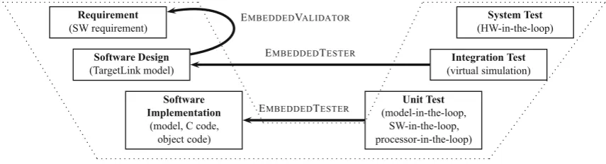
Fig. 1.Tool chain for embedded software development in the V model

2. Verification of model-based embedded software

Recent safety standards, e.g. ISO-26262 [ISO11], cover model-based development and testing techniques for early

simulation, testing and verification, and recommend back-to-back testing for showing simulation equivalence be-tween a high-level model and corresponding production code. In the automotive industry, model-based

develop-ment including automatic code generation is well-established. In particular, SIMULINK2for functional modelling and

TARGETLINK3for automatic code generation from these models are prominent representatives. SIMULINKDESIGN -VERIFIER,4 BTC EMBEDDEDTESTER,5 REACTIS,6 and RT-TESTER7 are exemplars of tools that complement the software development tool chain for formal verification of safety requirements against design models. These tools are also used for testing, namely, requirement-based and back-to-back testing, including automatic test vector generation for structural coverage criteria.8

An example of an embedding of this tool chain into the V model, the software development model suggested by

ISO-26262, is illustrated in Fig.1. Tools such as BTC EMBEDDEDVALIDATORsupport the automation of formally

verifying the requirements against the design model. On lower levels, automated test generation tools such as BTC EMBEDDEDTESTERhelp validate the implementation in the unit and integration test phases.

In this article, we focus on the verification of C code generated from these models. To this end, we illustrate

the characteristics of this verification problem with the help of a well-known case study (Sect.2.2) and explain the

workflow and principal techniques that a state-of-the-art verification tool for embedded software uses.

2.1. Requirements and challenges

In the setting above, verification tools have two main applications: (1) proving/disproving safety properties, and (2) covering test goals or proving their unreachability. BMC-based verification engines are a perfect fit for both

appli-cations because they can be used to find counterexamples and prove properties byk-induction. Fig.2illustrates the

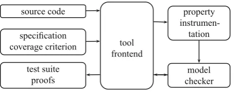
schematic architecture of such tools. They consist of a frontend that interacts with the user and a verification back-end that performs the actual analysis. To achieve good usability of such a tool, it is important to hide the underlying technical details of the verification backend from the user.

Verification tools, such as BTC EMBEDDEDVALIDATOR, target application (1). They take as inputs the source

code (or a design model) and a specification, typically a set of predefined properties, e.g. to check for common runtime errors such as overflows or division-by-zero, or user-defined properties that formalise functional requirements. The properties are then instrumented into the source code (or design model), typically on the level of an intermediate

representation. We will give an illustrative example for such an instrumentation in Sect.2.4. The instrumented code is

then checked by a model checker. The frontend reports to the user whether properties have been proved or disproved. In the latter case, the model checker provides a counterexample that is reported to the user for debugging.

2 _{http://www.mathworks.co.uk/products/simulink/}_.

3 _{http://www.dspace.com/en/pub/home/products/sw/pcgs/targetli.cfm}_. 4 _{http://uk.mathworks.com/products/sldesignverifier}_.

5 _{http://www.btc-es.de/index.php?lang=2}_. 6 _{http://www.reactive-systems.com}_. 7 _{https://www.verified.de/products/rt-tester}_.

(5)

tool frontend

source code property

instrumen-tation specification

coverage criterion

test suite proofs

[image:5.595.183.414.89.180.2]

model checker

Fig. 2.Typical architecture of a model checker for embedded software

Application (2) is addressed by test generation tools, e.g. BTC EMBEDDEDTESTER. Their input is the source code

and a coverage criterion, e.g. MC/DC (Modified Condition/Decision Coverage) [HVCR01]. MC/DC requires that test

executions reach not only each function entry and function exit and both outcomes of a decision (both branches of if-then-else), but they also have to show that each basic Boolean condition (that is part of a more complex Boolean decision) independently affects the outcome of the decision. Similar to properties, these coverage criteria are instru-mented into the code as test goals whose reachability is to be proven by the model checker. The counterexamples provided by the model checker are then transformed into a test suite and presented to the user.

Embedded C code has to meet many conflicting requirements like real-time constraints, low memory footprint and low energy consumption. Code generators offer options to perform certain optimisations towards these goals, often to

the detriment ofcode size(and also readability for humans). The observer instrumentation9 to encode properties and

identify the test goals corresponding to code-coverage criteria such as MC/DC produces a non-negligible overhead in the size of the code but introduces little semantic complexity. When using BMC, the size of the SAT formula built from a program further increases whenever internal loops need to be unwound. File sizes of 10 MB and more are common, which poses difficulties to many tools already when parsing the source code and encoding the program into a SAT formula, mostly due to inefficient data structures. Incremental BMC helps reduce formula sizes and peak memory

consumption (see Sect.4.2) by incremental formula generation and solving.

In practice, many loop unwindings may be needed to detect errors and reach certain tests goals (more than 100

for some of our industrial benchmarks, see Sect.4.2).Non-incremental bounded model checking repeats work such as

file parsing, loop unwinding, SAT formula encoding and discards information learnt in the SAT solver every time it is called and so gives away an enormous amount of performance. This effect exacerbates the cost of large unwinding limits that may be needed.

The main challenge addressed by this article is to exploit all the benefits of incrementality in BMC and to sig-nificantly enhance performance of its integration with an industrial-strength embedded verification and test-vector

generation tool, namely BTC EMBEDDEDVALIDATORand EMBEDDEDTESTER. The impact of this successful

tech-nology transfer is demonstrated on original industrial embedded software.

2.2. Case study: fault-tolerant fuel control system

The Fault-Tolerant Fuel Control System10(FUELSYS) for a gasoline engine, originally introduced as a demonstration

example for MATLAB SIMULINK/STATEFLOWand then adapted for dSPACE TARGETLINK, is representative of a

variety of automotive applications as it combines discrete control logic via STATEFLOW with continuous signal flow

expressed by SIMULINK or TARGETLINKand thus establishes a hybrid discrete-continuous system. More precisely,

the control logic of FUELSYSis implemented by six automata with two to five states each, while the signal flow is

further subdivided into three subsystems with a rich variety of SIMULINK/TARGETLINKblocks involving arithmetic,

lookup tables, integrators, filters and interpolation (Fig.3).

9 _{The observer instrumentation consists of adding a series of flags to the original source code that enables the analysis tool to determine exactly}

what parts of the code are exercised.

(6)

sensor correction airflow computation fuel computation

throttle • throttle throt est throt est

speed • speed speed est speed est air flow est air flow est

EGO • EGO EGO est EGO est

press • press

fail throt fail speed

failO2 fuelrate fuel rate

control logic fail press MAP est MAP est

throttle fail throt

speed failspeed fuelmode feedback corr feedback corr

EGO fail O2 • • fail O2

press fail press

clock clock fuel mode • fuel mode

[image:6.595.87.515.91.218.2]

fail O2

Fig. 3.The SIMULINKdiagram for the Fault-Tolerant Fuel Control System (without the plant model)

The system is designed to keep the air-fuel ratio nearly constant depending on the inputs given by a throttle sensor, a speed sensor, an oxygen sensor (EGO) and a pressure sensor (MAP). Moreover it is tolerant to individual sensor faults and is designed to be highly robust, i.e. after detection of a sensor fault the system is dynamically reconfigured.

Properties of interest. The key functional property for FUELSYSis that for each of the four sensor-failure scenarios the air-fuel ratio reaches a given range around a set target ratio within a given bounded time span. Simulation-based

approaches show that FUELSYS is indeed fault-tolerant in each case of a single failure: the air-fuel ratio can be

regulated after a few seconds to about80%of the target ratio. In addition tofunctionaltesting of industrial embedded

software, safety standards call forstructuraltesting of the production code before release deployment. In Sect.2.4, we

give a brief overview about such standards and the state of practice of their implementation in industry.

2.3. Structure of generated code

Many modelling languages follow thesynchronous programming paradigm [Hal93], which is well-suited for

mod-elling time-triggered systems, in which tasks (subsystems of the model) execute at given rates. Code generation for such languages produces a typical code structure, which corresponds essentially to a non-preemptive operating sys-tem task scheduler. Most code generators provide the scheduler for time-triggered execution or code to interface with popular real-time operating systems. In either case, the functionality corresponds to the following pseudo code:

1 void main ( ) {

2 s t a t e s ; i n p u t s i ; outputs o ;

3 i n i t i a l i z e ( s ) ;

4 while( t r u e ) { / / main l o o p

5 i = r e a d i n p u t s ( ) ;

6 ( o , s ) = compute step ( i , s ) ;

7 w r i t e o u t p u t s ( o ) ;

8 wait ( ) ; / / w a i t f o r t i m e r i n t e r r u p t

9 }

10 }

The distinguishing characteristic of such a reactive program is its unbounded main loop, which we will analyse incrementally. All other loops contained within that loop, e.g. to iterate over arrays or interpolate values using look-up tables, have a statically bounded number of iterations and can be fully unwound.

2.4. Analysis with BMC and

k

-induction

Property instrumentation. Formal verification requires formalisations of high-level requirements, often using

ob-server B¨uchi automata [Bue62] with a dedicated ‘error state’ generated from temporal logic descriptions. Test vector

generation is done for code-coverage criteria such as branches, statements, conditions and MC/DC of the production C

code. For FUELSYS, for example, MC/DC instrumentation yields251test goals. The properties to be verified or tested

(7)

To validate whether the air-fuel ratio in the FUELSYScontroller is regulated after a few seconds to be within some margin of the target ratio, one has to instrument the reactive program, as sketched above, with an observer implementing the asserted property. For instance, consider the requirement “If some sensor fails for the first time then within 10 s the air-fuel ratio will always stay between the range of 80–120% of the target ratio.” The code fragment for an observer for this requirement may look as follows:

1 / / d e t e c t i o n o f f i r s t s e n s o r f a i l u r e

2 i f ( s e n s o r f a i l == 1 && o b s e r v e r a t i o == 0 ) {

3 / / i n i t i a l i z e o b s e r v e r v a r i a b l e s

4 o b s e r v e r a t i o = 1 ;

5 c o u n t e r = 0 ;

6 v i o l a t e d = 0 ;

7 }

8 i f ( o b s e r v e r a t i o == 1 ) { / / o b s e r v a t i o n mode 9 i f ( c o u n t e r>= 10 &&

10 ( a i r f u e l r a t i o < 0 . 8∗t a r g e t r a t i o | |

11 a i r f u e l r a t i o > 1 . 2∗t a r g e t r a t i o ) )

12 v i o l a t e d = 1 ;

13 c o u n t e r ++;

14 }

15 a s s e r t ( v i o l a t e d == 0 ) ; / / s a f e t y p r o p e r t y

In order to verify that the above property actually holds, one has to show that the assertion in the observer code is

always satisfied. We use BMC for refutation of the assertion, andk-induction for proving it.

Bounded model checking. We model a reactive program, as given in Sect.2.3, as a transition system with initial

statesφ(functioninitialize) and a deterministic transition functionT : (s,i)→ sthat maps a states and an input

ito a resulting states(functioncompute step; w.l.o.g. we assume that the outputs are part of the state in order to

simplify the notation). BMC [BCCZ99,CBRZ01] can be used to check the existence of a pathπ s₀,s₁, . . . ,skof

lengthk between two statess₀ ands_k belonging to sets respectively described byφandψ. This check is performed

by deciding satisfiability of the following formula using a SAT or SMT solver:

φ(s0)∧ ⎛

⎝

0≤j<k

T(sj,ij,sj+1)

⎞

⎠_∧_ψ_(s_k₎ (1)

If the solver returns the answer “satisfiable”, it also provides a satisfying assignment to the variables(s₀,i₀,s₁,i₁, . . . ,

sk−1,ik−1,sk). The satisfying assignment represents one possible pathπ s0,s1, . . . ,skfromφtoψand identifies

the corresponding input sequencei₀, . . . ,ik−1. Hence, BMC is useful for refuting safety properties (whereφgives

the set of initial states andψdefines the error states) and generating test vectors (whereψdefines the test goal to be

covered). In the latter case, the initial states₀together with the input sequencei₀, . . . ,ik−1is a test vector.

Unbounded Model Checking by k-Induction. BMC can prove reachability, whereas unreachability can be shown

using induction. Let us first define the notion of an invariant. The predicate¬ψis an (inductive) invariant, i.e., it holds

in all reachable states, if each of the following two formulae, base case (BC) and induction step (SC), are valid.

(BC) ∀s:φ(s)⇒ ¬ψ(s)

(SC) ∀s,i,s:¬ψ(s)∧T(s,i,s)⇒ ¬ψ(s) (2)

The base case states that the initial state must be part of the invariant, and the step case ensures that all states are transitively reachable through the transition relation are also in the invariant. By negating each of the above formulae

we obtain an equivalent condition:¬ψis an invariant if the two following formulae are unsatisfiable.

(BC) ∃s :φ(s)∧ψ(s)

(SC) ∃s,i,s:¬ψ(s)∧T(s,i,s)∧ψ(s) (3)

(8)

The property of interest is often not inductive, however, and the check above fails. An option is to strengthen the property, e.g., using auxiliary invariants obtained using an abstract interpreter. Furthermore, the criterion above can be

generalised tok-induction [SSS00,ES03b,HT08,DHKR11]: The predicate¬ψis ak-inductive invariant, i.e., it holds

in all reachable states, if each of the following two formulae, base case (BC) and induction step (SC), are unsatisfiable

for a givenk(assuming that we have already checked for up tok−1):

(BC) φ(s₀)∧₀_≤_j_<_k¬ψ(s_j)∧T(s_j,i_j,s_j₊₁) ∧ψ(s_k)

(SC) ₀_≤_j_≤_k¬ψ(s_j)∧T(s_j,i_j,s_j₊₁) ∧ψ(s_k₊₁) (4)

The base case checks if the formula is unsatisfiable, when this occurs we say that¬ψholds in the firstk steps. The

induction step checks if we can conclude from the invariant holding over anykconsecutive steps that it holds for the

(k+ 1)st _{step. If the base step fails, i.e. above formula is satisfiable and a counterexample is given, we have refuted}

the property. If the base case holds and the induction step fails, we do not know whether¬ψis invariant. Only if both

formulae hold we have proved that¬ψis invariant.

Both base step and induction step are essentially instances of BMC: starting from the initial stateφfor the base

case, and starting fromanystate for the induction step. Thus, similar to BMC,k-induction can be applied by using a

sequence of increasing values fork.

3. Incremental BMC

In this section, we explain the technical background of incremental SAT solving and how it is employed in our imple-mentation of incremental BMC.

3.1. Incremental SAT solving

The first ideas for incremental SAT solving date back to the 1990s [Hoo93,SS97,KWSS00]. The question is how

to solve a sequence of similar SAT problems while reusing effort spent on solving previous instances. The authors of [Str01,WKS01] identify conditions for the reuse of learnt clauses, but this requires expensive book-keeping, which partially saps the benefit of incrementality. Obviously, incremental SAT solving is easy when the modification to the CNF representation of the problem makes it grow monotonically. This means that if we want to solve a sequence of

(increasingly constrained) SAT problems with CNF formulae(k)fork ≥0then(k)must begrowing

monotoni-callyink, i.e.(k+ 1) (k)∧ϕ(k)for CNF formulaeϕ(k). Removal of clauses from(k)is trickier, as some of the clauses learnt during the solving process are no longer implied by the new instance, and need to be removed

as well. This requires additional solver features like solvingunder assumptions[ES03b], which is the most popular

approach to incremental SAT solving: assumptions are temporary assignments to variables that hold solely for one

specific invocation of the SAT solver. We will see that incremental BMC requires anon-monotonicseries of formulae.

In Sect.3.2, we will explain how SAT solving under assumptions allows us to emulate the removal of clauses.

An alternative approach is to use SMT solvers. SMT solvers offer an interface for pushing and popping clauses in a stack-like manner. Pushing adds clauses, popping removes them from the formula. This makes the modification of the formula intuitive to the user, but the efficiency depends on the underlying implementation of the push and pop

operations. For example, in [GW14] it was observed that some SMT solvers (like Z3) are not optimised for incremental

usage and hence perform worse incrementally than non-incrementally.

The bounded model checker that we are using, CBMC[CKL04], itself implements powerful bitvector decision

procedures that use a SAT solver such as MINISAT2 [ES03a] as a backend solver. For SAT solvers, solving under

assumptions is the prevalent method, hence we will focus on this technique in the sequel.

3.2. Incremental BMC

(9)

Following the construction in [ES03b] for finite state machines, incremental BMC can be formulated as a sequence

of SAT problems(k)that we need to solve:

(0) :φ(s0)∧((0)∨α0)

with assumption¬α0

(k+ 1) :(k)∧T(sk,ik,sk+1)∧αk∧((k+ 1)∨αk+1)

with assumption¬αk+1

(5)

where(k)is the disjunction₀_≤_j_≤_kψ(sj)of error statesψ(sj)to be proved unreachable up to iterationk. This

disjunction means that the verification fails ifat least oneof the error states is reachable. Since the number of disjuncts

in the disjunction₀_≤_j_≤_kψ(s_j)grows in each iteration, our problem is not monotonic: one has toremove(k)when

adding(k+1)because(k)subsumes(k+1). This issue can be solved with the help ofsolving under assumptions.

In iterationk, theαkis assumed to be false, whereas it is assumed true for iterationsk>k. This has the effect that in

iterationkthe formula((k)∨αk)becomes trivially satisfied. Hence, it does not contribute to the (un)satisfiability

of(k), which emulates its deletion.11

Symbolic execution. In the case of software analysis, the unfolding scheme (5) results in large formulae and would

be highly inefficient. In practice, software model checkers usesymbolic executionin order to exploit, for example,

constant propagation and pruning branches when conditionals are infeasible, while generating the SAT formula and

thus reducing its size. This means that the formula describingTis the result of symbolic execution, and that formulae

Tandare actually dependent onk. Fortunately, this does not affect the correctness of the above formula construction

and we can replaceT byTkin (5) andψbyψkin the definition of(k).Tkdenotes the transition formula obtained

by symbolic execution of thekth_{time frame (i.e. unwinding), and}_ψ

kthe assertions collected for this time frame.

Slicing. Another feature used by state-of-the-art software model checkers is slicing: The purpose of slicing is, again, to reduce the size of the SAT formula by removing (or better: not generating) those parts of the formula that have no influence on its satisfiability. There are many techniques how to implement slicing with the desired trade-off between

runtime efficiency and its formula pruning effectiveness [HH01,Tip94].

Slicing is performed relative to(k). We know that the number of disjunctsψ(s_j)inis growing monotonically

withk. Hence, we will show that, assuming that our slicing operator is monotonic, we obtain a monotonic formula

construction:

The transition formulaTk for each time frame k obtained by symbolic execution is a conjunction

τ∈Mτ of

subrelationsτ (e.g., formulae corresponding to program instructions). We useM to denote the set of these subrelations

τ. The slicing operatorsli ceselects a subset ofM. The operatorsli ceis monotonic iff for all sets of subrelations

M1,M2the following holds:M1⊆M2⇒sli ce(M1)⊆sli ce(M2).

We can then view the conjunction of transition relations forktime framesT(k )₀_≤_j_≤_kT_j as_τ_∈_M

kτ. A slice

Tsliced_(k) _of _T_(k) _is

τ∈Mk τ where M

k ⊆ Mk. An incremental slice is then defined as the difference between

Tsliced_(k_{+ 1)}_and_Tsliced_(k)_:

Tsliced k+1

τ∈M_k₊₁\M_k

τ. ₍₆₎

Monotonicity of the formula construction follows fromM_k₊₁ ⊆ M_k₊₁ and the assumed monotonicityM_k ⊆M_k₊₁

of the slicing operator. We can thus replaceT byT_ksliced in (5). It is worth mentioning thatT_ksliced also contains the subrelationsτ for time stepsk<k.

Our slicing operator computes the (syntactic) variable dependency graph forT(k + 1)and obtainsM_k₊₁ as the

set of allτ which(k+ 1)depends on. Moreover, it takes into account that conditionals could trivially evaluate to

false after constant propagation and thus the corresponding branches are not reachable. Then only thoseτ inM_k₊₁are

added to the formula that have not been in the slice for the previous time frame, resulting inTsliced

k+1 .

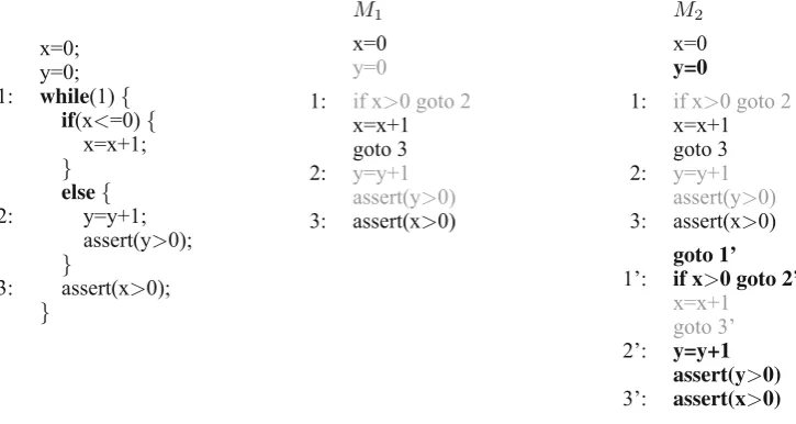
We give an example in Fig.4. The middle and right-hand side columns give the instructions that are transformed

into sets of subrelationsM₁andM₂in order to build the transition relationT. Note that these subrelations correspond

to the simple program on the left-hand side column. The sets of subrelationsM₁andM₂are obtained from the

non-greyed instructions in the middle and right-hand side column, respectively. The incremental sliceT₂sli ced is built from

M

2\M1, which corresponds to the bold instructions in the right-hand side column. Note that this incremental slice

takes into account a subrelation (corresponding to instruction y=0) that is inM1, but not inM₁.

11 _{For a large number of iterations}_k_{, such trivially satisfied subformulas might accumulate as “garbage” in the formula and slow down its resolution.}

(10)

x=0; y=0; 1: while(1){

if(x<=0){ x=x+1;

} else{

2: y=y+1; assert(y>0);

}

3: assert(x>0);

}

M1

x=0

y=0

1: if x>0 goto 2

x=x+1 goto 3 2: y=y+1

assert(y>0)

3: assert(x>0)

M2

x=0

y=0

1: if x>0 goto 2

x=x+1 goto 3 2: y=y+1

assert(y>0)

3: assert(x>0)

goto 1’

1’: if x>0 goto 2’ x=x+1 goto 3’

2’: y=y+1 assert(y>0)

[image:10.595.118.481.92.285.2]

3’: assert(x>0)

Fig. 4.Incremental slicing

3.3. Incremental refinements

Incremental SAT solving is also used for incremental refinements of the transition relationT for bitvectors and arrays.

Bitvector refinement. The purpose of bitvector refinement [BKO+07,Bie08,HH08,BKO+09,BB09c,EMA10] is to reduce the size of formulae encoding bitvector operations. This is especially important for arithmetic operations that generate huge SAT formulae, e.g. multiplication, division and remainder operations, both for integer and

floating-point variables [BKW09]. Bitvector refinement is based on successive under- and over-approximations. For instance,

under-approximations can be obtained by fixing a certain number of bits, whereas over-approximation make a certain number of bits unconstrained. If an under-approximation is satisfiable (SAT) or an over-approximation is unsatisfiable (UNSAT) we know that the non-approximated formula is SAT or UNSAT respectively. Otherwise, the number of fixed respectively unconstrained bits is reduced until the non-approximated formula itself is checked.

Arrays. To handle programs with arrays, Ackermann expansion is necessary to ensure the functional consistency

property of arrays:∀i,j :i j ⇒A[i]A[j]. However, adding a quadratic number of constraints (in the size of

the arrayA) is extremely costly. Experience has shown that only a small number of these constraints is actually used

[PS06].

Hence, it is more efficient trying to solve the SAT formula without these constraints, which is an over-approximation. Hence, if we get an UNSAT result (a), we know that the solution with the Ackermann constraints would be UNSAT, too. In case of a SAT result (b), we check the consistency of the obtained model: if it turns out not to violate consistency, then we know that we have found a real bug. Otherwise (c), we add the violated Ackermann constraint to the formula. The formula construction is trivially monotonic and we can use incremental SAT solving. We repeat the procedure until we hit case (a) or (b), which is guaranteed to happen. Some SMT solvers, such as BOOLECTOR, implement a similar procedure to decide the SMT-LIB array theory [BB09a,BB09b].

Formula construction. Applying above refinements inside an incremental Bounded Model Checker requires using several incremental formula encodings for (in general, non-monotonic) refinements simultaneously. These refinements

are global over all unwindings, so that in iterationk we have to further refine transition relations Tk from earlier

iterationsk<k. We can formalise the incremental formula construction as follows: For iterationk ≥0of incremental

BMC and theth_refinement:

(0,0) :φ(s0)∧(0(s0)∨α0)

with assumption¬α₀

(k+ 1, ) :(k, )∧(k+1(sk+1)∨αk+1)∧αk∧

T

k+1,(sk,ik,sk+1)∨β

with assumptions¬αk+1and¬β

(k, + 1) :(k, )∧T

k−1,+1(sk−1,ik−1,sk)∨β+1∧β

with assumptions¬αkand¬β+1

fork≥1

(11)

The counteris incremented in each iteration of the refinement loop until convergence, whereaskis incremented when considering the next time frame. The formulasαk are the assumptions for the incremental extension of the time frames, whereas the formulasβare the assumptions for the refinement iterations.

4. Experimental evaluation

We present the results of our experimental evaluation of incremental BMC and incrementalk-induction on industrial programs mainly from the automotive industry. The goal of this evaluation is to quantify the benefit from an incremental approach in a BMC-based tool infrastructure.12_{The experiments described in Sects.}_4.2_,_4.2_and_4.4_{were performed on a 3.5 GHz Intel Xeon machine with 32 GB of} physical memory running Windows 7 with a time limit of 3600 s. The evaluation on programs with multiple loops (Sect.4.5) was run on the StarExec [SST14] cluster infrastructure on 2.40 GHz Intel Xeons running Red Hat Enterprise Linux Workstation release 6.3 (Santiago) with a timeout of 1800 s and a memory limit of 32 GB.

4.1. Implementation

CBMC. We implement our extension13_{for incremental BMC in the Bounded Model Checker for ANSI-C programs C}_BMC_[_CKL04_{] using} the SAT solver MINISAT2 [ES03a]. CBMCis called in incremental mode using the command linecbmc file.c --incremental. There is an optimised option for programs with a single unbounded loop (see Sect.4.2). The following options can be added to enable specific features of CBMC:

• --no-sat-preprocessor: turns off SAT formula preprocessing, i.e. the MINISAT2 simplifier is not used. • --slice-formula: slices the SAT formula.

• --refine: enables bitvector refinement.

• --unwind-max k: limits the unwindings of the loop to be checked incrementally tokunwindings. Without this option, CBMCwill not terminate for unsatisfiable instances, i.e. bug-free programs with unbounded loops.

Incremental CBMCcan be used with specific options that enables extra features, namely: (i) slicing, (ii) preprocessing, and (iii) formula-level refinements. The goal of these techniques is to reduce the size of the SAT formula that is being generated. Slicing reduces the size of the SAT formula by eliminating irrelevant paths of the program. Preprocessing through the MINISAT2 simplifier reduces the size of the SAT formula after it has been generated, and formula-level refinements perform an incremental build of the SAT formula. More information regarding the usage of incremental CBMCcan be found on the CPROVER wiki page14_.

Integration with an industrial-strength embedded verification tool. In the integration of CBMCwith BTC EMBEDDEDTESTERand EMBEDDEDVALIDATOR, a master routine selects the next verification/test goal to be analysed starting from instrumented C code. After some preprocessing like source-level slicing and internal-loop unwinding the resulting reachability task is given to CBMC. If CBMCis able to solve the problem within the user-defined time limit, the result, i.e. bounded or unbounded unreachability, or a counterexample in case of reachability, is reported back to the master process. Otherwise, i.e. in case of a timeout, the CBMCprocess is terminated but information about the solved unwindings of the reactive main loop is returned, which frequently is a useful result for the user since it may indicate the absence of shallow bugs.

To prove unreachability of verification/test goals (properties),k-induction is performed (see Sect.2.4). For this purpose BTC EMBED -DEDTESTERgenerates two source files, one containing the base case, which is a normal BMC problem with the property given as assertion (cf. Eq. (4) (BC)); in the file for the step case, the variables modified in the loop are havocked, i.e., they are assigned a nondeterministic value at the beginning of the loop. Then the invariant property is assumed, and at the end of the loop the invariant property is asserted (cf. Eq. (4) (SC)). By default, CBMCstops when a counterexample for a property is found, but to check the step case, we require a reversed termination behaviour of CBMC, (option--stop-when-unsat), i.e. CBMCcontinues unwinding as long as the problem is SAT and stops as soon as it is UNSAT.

Implementation of Incremental BMC for General Sequential Programs. Incremental CBMCcan also be used for programs with multiple loops. For these programs, CBMCincrementally unwinds loops one at each time. For each loop, the incremental procedure is similar to the one described in Sect.3.2for a single unbounded loop. For programs with multiple loops, CBMCwill unwind each loop until it is fully unwound or until a maximum depthkis reached. We can detect that a loop is fully unwound at unwindingj <kif all states reached at unwindingjdo not satisfy the loop condition. After a loop has been unwound, CBMCcontinues to the next loop. This procedure is repeated until all loops have been unwound or a bug has been found. Recursive function calls are treated similarly.

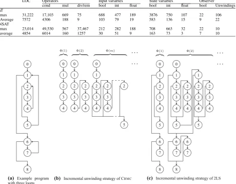
Consider the control flow graph (CFG) in Fig.5(a). The unwinding strategy is illustrated for this CFG in Fig.5(b). The program has three loops with loop heads 1, 2 and 6 (2 is nested inside 1). The symbolic execution that generates the incremental BMC formula(k)(see Sect.3.2) traverses the CFG and stops each time when it encounters an edge in the CFG that returns to a loop head (a so-calledback-edge). Fig.5(b) shows three snapshots of the partially unwound CFG that correspond to the parts of the program considered by instances of the incremental BMC formula(k)fork 1,2,m. We write(1)for the formula up to the first back-edge encountered that returns to the loop head of the inner loop (2). Formula(2)extends(1)by one further unwinding of the inner loop.

12 _{For a comparison with alternative verification approaches, we refer to the results of the Software Verification Competition}

(http://sv-comp.sosy-lab.org), where BMC-based tools rank in the top 3 every year.

(12)

[image:12.595.74.535.107.465.2]

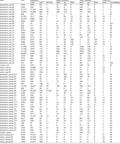
Table 1.Benchmark characteristics of industrial programs

LOC Operators Input variables State variables Observer

cond mul div/rem bool int float bool int float bool Unwindings SAT

max 31,222 17,103 669 75 688 477 189 3876 750 107 22 106

Average 7572 4306 188 9 103 79 19 583 136 15 9 22

UNSAT

max 23,014 49,530 567 37,467 212 282 188 708 663 32 22 10

average 4854 6014 160 1257 30 51 9 163 73 3 7 10

0 1 2 3 4 5 6 7 8

(a) Example program

with three loops

Φ(1) Φ(2) Φ(m)

_{. . .}

. . .

0 1 2 3 4 0 1 2 3 4 2 3 4 0 1 2 3 4 2 3 4 2 5

(b) Incremental unwinding strategy of CBMC

Φ(1) Φ(2)

_{. . .}

. . .

0 1 2 3 4 5 6 7 8 0 1 2 3 4 2 3 4 5 6 7 6 7 8 1 2 3 4 2 3 4 5

(c) Incremental unwinding strategy of 2LS

Fig. 5.Incremental unwinding strategies

Assume thatmis the maximum number of unwindings of the inner loop, then(m)shows the extension of the formula to the case where the inner loop has been unwound up to this maximum number within the first iteration of the outer loop (with loop head 1). Formula (m+ 1)will then extend(m)by a first unwinding of the inner loop (up to program location 4) for the second iteration of the outer loop. This process continues until a failed assertion or the end of the program (8) is reached.

Implementation of Incremental BMC in 2LS. We implement a different approach to incremental BMC in the static analysis tool 2LS [SK16,BJKS15].15_{2LS unwinds}_all_loops_k_{times and incrementally adds the}₍_k_{+ 1)}_{th for}_all_{loops instead of unwinding only the} first loop encountered until it has been fully unwound.

We illustrate this unwinding strategy in Fig.5(c), which shows the first two partial unwindings of the CFG in Fig.5(a) that correspond to(1)and(2), respectively. Formula(1)consists of one unwinding (up to, but not including the back-edge) for the loops 1, 2, and 6. Formula(2)then adds another unwinding to each loop. Note that we have two times two unwindings of the inner loop (with loop head 2) now, two for each unwinding of the outer loop (loop head 1).

Structurally, this unwinding strategy is the same as the one that we use in non-incremental CBMC when calling with fixed values fork. In comparison with incrementally unwinding a single loop, the incremental extension of the formula fromktok+ 1unwindings in Eq. (5) is now also non-monotonic because ofT(and not only because of). This renders many optimisations that non-incremental CBMC performs during symbolic execution such as constant propagation impossible.

(13)

0 1 2 3 4 5

ni

ni+s

ni+s+p

ni+s+p+r

i

i+s

i+s+p

i+s+p+r

average speedup

(a) Effect of slicing, SAT formula preprocess-ing and bitvector refinement

10-1 100 101 102 103 104

ni+s+p

i+s+p 10x speedup

10x slowdown

3600 sec. timeout

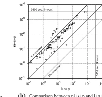
[image:13.595.135.463.82.252.2] [image:13.595.292.461.88.249.2]

(b) Comparison between ni+s+p and i+s+p (+SAT instances; UNSAT instances)

Fig. 6.Incremental versus non-incremental BMC

4.2. Incremental BMC for embedded software

We report results on industrial programs for the integration of CBMCwith BTC EMBEDDEDTESTERand EMBEDDEDVALIDATOR. For these experiments, we used 60 industrial benchmarks, which are original, unmodified code from BTC customers, mainly from automotive applications. Unfortunately, software in the automotive domain is closed source, and hence, being subject to NDAs, these benchmarks cannot be made public.16_{These benchmarks have exactly one unbounded loop. Half of the benchmarks are bug-free (UNSAT instances),} half contain a bug (SAT instances). This benchmark suite is suitable for evaluating the performance of model checking tools in an industrial setting as it covers a representative spectrum of embedded software.

A summary of the benchmark characteristics is listed in Table1. Besides the number of lines of code, we give the number of conditional operators, multiplications and divisions or remainder operations, which are a good indicator for the difficulty of the benchmark, because they generate large formulae — for instance, for each “/” occurring in the program, CBMChas to generate a divider circuit. The surprisingly high number of conditional operators in most of the benchmarks is due to the preprocessing of conditional assignments by BTC EMBED -DEDTESTERand hints at the amount of branching in these benchmarks. Moreover, we list the number of input and state variables, and the variables introduced by the observer instrumentation.

For these benchmarks, CBMCis called in incremental mode by using the option--incremental-check main.0wheremain.0 is the loop identifier of the unbounded loop to be unwound and checked incrementally. The loop identifiers can be obtained using the option --show-loops.

Runtimes. We compared the incremental (i) with the non-incremental (ni) approach and evaluated the impact of slicing (s), SAT prepro-cessing (p) and bitvector refinement (r).17_{The incremental and non-incremental approaches were compared by activating none of the three} techniques, with slicing only (+s), with slicing and preprocessing (+s+p), and with all three options activated (+s+p+r). The maximum number of loop unwindings was fixed to 10 for the UNSAT instances in order to balance a significant exploration depth with reasonable analysis runtimes. For SAT instances, a maximum number of loop unwindings was not fixed since the incremental and non-incremental approaches are bound to terminate when the unwinding depth reaches the depth of the bug. The number of unwindings are listed in the last column in Table1.

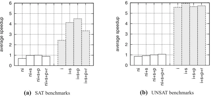
Fig.6a gives the average geometric mean [FW86] speedup of instances that were solved by all approaches. Fig.7provides these results split into SAT and UNSAT instances. We consider the (ni+s+p) approach as the baseline since it is the best non-incremental approach. Each bar gives the average geometric mean speedup of each approach when compared to (ni+s+p). For example, (ni) has a speedup of 0.77, i.e., (ni) is on average 0.77×as fast as (ni+s+p). On the other hand, all incremental versions are much faster than the non-incremental versions. For example, (i) is on average over 3.5×faster than (ni+s+p) and (i+s+p) is on average over 5×faster than (ni+s+p). We observe the following effects of the tool options: (i) slicing shows significant benefits overall (also on peak memory consumption), although the effect is less significant for UNSAT than for SAT instances; (ii) not using formula preprocessing is a bad idea in general; and (iii) bitvector refinement provides benefits for UNSAT instances, but produces the overhead for SAT instances, which deteriorates the overall performance of the tool (see Fig.7(a)). Even though the tool options have some positive effects, they are minor in comparison to the performance gains from using the incremental approach.

Since the best incremental and non-incremental approaches were obtained with the configuration (+s+p), we will use this configuration for both approaches for the results described in the remainder of the article.

(14)

0 1 2 3 4 5 6

ni

ni+s

ni+s+p

ni+s+p+r

i

i+s

i+s+p

i+s+p+r

average speedup

(a) SAT benchmarks

0 1 2 3 4 5 6

ni

ni+s

ni+s+p

ni+s+p+r

i

i+s

i+s+p

i+s+p+r

average speedup

[image:14.595.131.472.90.248.2]

(b) UNSAT benchmarks

Fig. 7.Effect of slicing, SAT formula preprocessing and bitvector refinement

Incremental BMC: 27% % 2151s

Non-incremental BMC: 28% % 11,811s

Last iteration of non-incremental BMC: 784s 7 3317s

Fig. 8.Solving time versus overall runtime

Fig.6b is a scatter plot with runtimes of the best non-incremental (ni+s+p) and incremental (i+s+p) approaches. Each point in the plot corresponds to an instance, where the x-axis corresponds to the runtime required by the incremental approach and the y-axis corresponds to the runtime required by the non-incremental approach. If an instance is above the diagonal, then it means that the incremental approach is faster than the non-incremental approach, otherwise it means that the non-incremental approach is faster. SAT instances are plotted as crosses, whereas UNSAT instances are plotted as squares. Incremental BMC significantly outperforms non-incremental BMC. For SAT instances, the advantage of incremental BMC is negligible for the easy instances, whereas speedups are around a factor of 10 for the medium and hard instances. For UNSAT instances, speedups are also significant and most instances have a speedup of more than a factor of 5.

Solving vs. overall runtime. Since CBMCis used as a black-box with BTC EMBEDDEDTESTERand EMBEDDEDVALIDATOR, the non-incremental approach has to re-parse files in each iteration. One might argue that removing this overhead is the main reason for the speedup observed. However, the overhead for parsing files, symbolic execution and slicing when compared to generating and solving SAT formula is similar for the incremental and non-incremental approach: 27% of the time taken by the incremental approach are spent in solving the SAT formula (582 out of 2151 s), compared with 28% of the time taken by the non-incremental approach (3317 out of 11,811 s). We illustrate this observation in the bar chart in Fig.8, which plots the total runtime consisting of the time spent in generating the SAT formula and solving it (light grey) and the overhead (dark grey) for incremental and non-incremental BMC. Unsurprisingly, as shown in the third bar in Fig.8, solving the instance for the largestkin the non-incremental approach (white) takes a considerable amount of time (around 24%), when compared to the total time (white+grey) for solving the SAT formulae for iterations 1 to k (784 out of 3317 s).

An explanation for these speedups might be the size of the queries issued in both approaches. The average number of clauses per solver call is halved from 1367k clauses for the non-incremental approach to 709k clauses for the incremental approach. Similarly, the average number of variables is less than a third in the incremental approach when compared to the non-incremental approach, being 217 and 746k respectively.

Peak memory consumption. Smaller query sizes also have an effect on peak memory consumption, which is reduced by 30% for UNSAT benchmarks; for SAT benchmarks, however, we observed a 10% increase.

4.3. Code coverage on

F

UEL

S

YS

using BTC E

MBEDDED

T

ESTER

(15)

10-2 10-1 100 101 102

Non-Incremental

[image:15.595.220.374.84.238.2]

Incremental

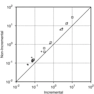
Fig. 9.Incrementalk-induction (+BC instances;2SC instances)

10-1 100 101 102 103 104

10-1 100 101 102 103 104 10x speedup

10x slowdown

1800 sec. timeout

Non-Incremental

[image:15.595.220.374.270.416.2]

Incremental

Fig. 10.Incremental versus non-incremental BMC on the SystemC category (+SAT instances;2UNSAT instances)

4.4. Incremental

k

-induction for embedded software

To compare the performance of incremental and non-incremental approaches fork-induction, we considered the subset of UNSAT bench-marks for whichk-induction required more than 1 iteration. Note that whenk-induction requires only 1 iteration, the performance of both approaches is similar.

Figure9shows a scatter plot with the runtimes of incremental and non-incrementalk-induction using the tool options (+s+p). Instances that correspond to the base case are plotted as crosses, whereas instances that correspond to the step case are plotted as squares. The runtimes for both incremental and non-incremental checking are relatively small. These are due to the small number of iterations required byk-induction to prove the unreachability of the properties present on these benchmarks (between 2 and 4 iterations with an average of 2.4 iterations per instance). Incremental checking is on average 2×faster than non-incremental checking, on both base and step cases.

4.5. Incremental BMC for programs with multiple loops

Incremental BMC is not restricted to programs with a single loop and may also be applied to programs with multiple loops. To evaluate the performance of incremental BMC on this kind of program, we compared the performance of incremental and non-incremental approaches on the 62 benchmarks from the SystemC category of the Software Verification Competition benchmark set,18_{because these benchmarks,} which were derived from SystemC models [CMNR10], contain many loops. Of these benchmarks, 25 are bug-free (UNSAT instances) and 37 contain a bug (SAT instances). These benchmarks have between 2 and 19 loops with an average of 10.3 loops per instance. For SAT instances, the depth of the bug ranges from 1 to 5 with an average depth of 2.5. When compared to industrial benchmarks, SystemC benchmarks are smaller and have shallow bugs, which illustrates some of the differences between industrial and academic benchmarks. For more details on these benchmarks see Table3in the “Appendix B”.

(16)

10-1 100 101 102 103 104

10-1 100 101 102 103 104 10x speedup

10x slowdown

1800 sec. timeout

Non-Incremental

Incremental

(a) Incremental vs. non-incremental BMC on additional loop bench-marks (+SAT instances; UNSAT instances)

10-1 100 101 102 103 104

10-1 100 101 102 103 104 10x speedup

10x slowdown

1800 sec. timeout

Non-Incremental

2LS

[image:16.595.117.475.90.241.2]

(b) 2LS vs. non-incremental BMC on additional loop benchmarks (+SAT instances; UNSAT instances)

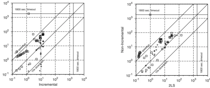
Fig. 11.Incremental and 2LS versus non-incremental BMC on additional loop benchmarks

We have fixed the maximum number of loop unwindings to 10 for both SAT and UNSAT instances. Note that this unwind depth is larger than the depth of the bugs for the SAT instances. Formula slicing is not yet fully supported in incremental CBMCfor programs with multiple loops, and has been disabled for the incremental approach.

Fig.10gives a scatter plot with the runtimes of the incremental and non-incremental approaches for SystemC benchmarks. For the majority of the instances, the incremental approach outperforms the non-incremental approach and for many SAT and UNSAT instances the speedup is larger than a factor of 10. However, there are a few instances for which the non-incremental approach performs better. The non-incremental approach unwinds all loops until a fixed unwind depth, whereas the incremental approach fully unwinds one loop before continuing to the next loop. For some instances, fully unwinding each loop may result in the generation of larger formulae, particularly for SAT instances. Not using slicing for the incremental approach may also result in larger formulae. The increase in formula size may explain the observed slowdown for some instances. Overall, when considering instances solved by both approaches, the incremental approach is faster than the non-incremental approach and the average geometric speedup is larger than a factor of 3.

Comparison with 2LS. We compared the incremental BMC implementations of CBMC and 2LS with non-incremental CBMC on 83 benchmarks from the Software Verification Competition benchmark set (categories Simple and Control Flow). These benchmarks are representative for general, i.e. transformational rather than reactive, programs. Most of these programs have only one loop, but the assertion is outside the loop, which distinguishes them from the embedded benchmarks. For more details on these benchmarks see Table4in the “Appendix C”.

Figure11presents the results. Although incremental CBMC is an order of magnitude faster than non-incremental CBMC on many benchmarks, there is a number of SAT benchmarks on which incremental CBMC is significantly slower than the non-incremental version (Fig.11a). The reason for this is that the unwinding strategy implemented in incremental CBMC is optimised for embedded software with a single unbounded loop (and with the assertions inside the loop). By contrast, this behaviour cannot be observed when comparing 2LS with non-incremental CBMC (Fig.11b). Although 2LS is slower than incremental CBMC on many benchmarks, the unwinding strategy of 2LS is advantageous for benchmarks where bugs “after” loops can be found with low numbers of unwinding. On such benchmarks 2LS clearly outperforms incremental CBMC and non-incremental CBMC.

We illustrate this observed behavioural difference on the example in Fig.5(a). Let us assume that the assertion is at program location 3 and that it fails in the third iteration of the inner loop of the first iteration of the outer loop. In this case incremental CBMC can find the bug by only unwinding a very small part of the program that considers only one unwinding of loop 1 and three unwindings of loop 2. By contrast, 2LS constructs a formula that has three unwindings of each loop (and actually nine instances of the inner loop!), which results in a large formula that slows down 2LS in comparison with incremental CBMC. On the other hand, let us assume that the assertion is at program location 8 and that it fails without entering any of the loops. Then the unwinding strategy of 2LS can find the bug in formula(1), whereas the unwinding strategy of incremental CBMC first has to unwind all the loops up to their maximum number of iterations before it is able to reach location 8.

5. Related work

Most related is recent work on a prototype toolNBIS[GW14], which implements incremental BMC using SMT solvers. They show the advantages of incremental software BMC. However, they do not consider industrial embedded software and have evaluated their tool only on small benchmarks that are very easy for both incremental and non-incremental approaches (runtimes<1 s).19

(17)

Bit-precise formal verification techniques are indispensable for embedded system models and implementations, that have low-level, i.e. C language, semantics like discrete-time SIMULINKmodels. The importance of this topic has recently attracted attention as shown by publications on verification using SMT Solving [HRB13,MMBC11], test case generation [PRS+12], symbolic analysis for improving simulation coverage [AKRS08], and directed random testing [SYR08]. Yet, all these works have not exploited incremental BMC.

The test vector generation tool FSHELL[HSTV09] uses incremental SAT solving to check the reachability of a set of test goals. However, it assumes a fixed unwinding of the loops. There is no reason why incremental BMC should not boost its performance when increasing loop unwindings need to be considered. Test vector generation tools like KLEE[CDE08] use incremental SAT solving to extend the paths to be explored. However, they consider only single paths at a time, whereas BMC explores all paths simultaneously.

Incremental SAT solving has important applications in other verification techniques like the IC3 algorithm [Bra12, EMB11] and incremental BMC is standard for hardware verification [JS05,Wie11]. We show that the speedups of incremental SAT solving reported in [ES03b] regardingk-induction on small HW circuits carry over to industrial embedded software.

6. Conclusions and future work

We claim that incremental BMC is an indispensable technique for industrial embedded software verification based on BMC. To underpin this claim, we report on the successful integration of our incremental extension of CBMCinto an industrial embedded software verifica-tion tool. Our experiments demonstrate one-order-of-magnitude speedups from incremental approaches on industrial embedded software benchmarks for BMC andk-induction. These performance gains result in faster property verification and higher test coverage, and thus, a productivity increase in embedded software verification.

Incremental BMC is effective on embedded software because of its specific properties (one big unbounded loop, whereas other loops are bounded). Nonetheless, we can also expect benefits for general software where loops and control structures are more irregular. We implement support for incremental BMC for programs withmultiple loopsin two tools, using different loop unwinding strategies. Our experimental evaluation shows that the version of incremental BMC implemented in CBMC works well on programs with multiple loops that are akin to embedded programs, whereas 2LS’s approach is better suited for general programs. Even though the engineering aspects of both approaches for multiple loops can still be improved, we already observe significant speedups in comparison to the non-incremental approach that show the applicability of incremental BMC beyond embedded software.

There are several opportunities to further improve the performance of BMC andk-induction for embedded programs in practice. It is often difficult to find bugs that require many unwindings using BMC because of the exponentially increasing amount of time and memory necessary to solve the generated SAT formulae. Kroening et al. [KLW15] present aloop accelerationtechnique that is sound for BMC, i.e. it adds short-cut paths to the program that have the effect of many loop iterations without introducing spurious behaviour. We would like to investigate how this technique can be combined with incremental BMC.

It has been shown [BDW15,BJKS15] that powerful verification tools can be built by strengthening the step case ink-induction with additional invariants that are inferred using abstract interpretation techniques. This approach can be further extended by using incremental loop unwindings [BJKS15]. However, a comprehensive study on the practical benefit for embedded programs has not yet been conducted. Regarding general programs, we are planning to implement support for recursion in 2LS so that we can compare it with incremental unfolding of recursions in CBMC. Also, we would like to add a slicing operator that supports multiple loops and recursion.

A promising application of incremental BMC is the analysis of concurrent programs through sequentialisations (e.g. [ITF+14]). In-crementality could be exploited in two ways in this context: by incrementally increasing the number of unwinding of loops (which might also augment the number of threads) and for increasing the number of context switches that are considered. The challenge is to find good encodings of these sequentialisations that allow us to use incremental SAT solving efficiently.

Open Access This article is distributed under the terms of the Creative Commons Attribution 4.0 International License (http://creativecommons.org/licenses/by/4.0/), which permits unrestricted use, distribution, and reproduction in any medium, provided you give appropriate credit to the original author(s) and the source, provide a link to the Creative Commons license, and indicate if changes were made.

Appendix A: Industrial benchmark characteristics

See Table2.

Appendix B: SystemC benchmark characteristics

See Table3.

Appendix C: Additional loop benchmarks characteristics

(18)

[image:18.595.70.534.126.683.2]

Table 2.Embedded software benchmark characteristics (name of the benchmark and application domain, lines of code, number of operators (cond(a?b:c), mul(*), div/rem(/,%)), number of boolean/integer/floating point input and state variables, number of boolean variables introduced by the observer instrumentation, number of loop unwindings considered; k-induction was performed on the instances marked with *)

Name LOC Operators Input variables State variables Observer

cond mul div/rem bool int float bool int float bool Unwindings

automotive sat 01 3762 2032 82 1 14 282 0 229 50 0 3 12

automotive sat 02 1854 189 79 1 78 4 0 165 7 0 3 15

automotive sat 03 15,277 17,103 669 75 230 244 0 868 275 0 1 9 automotive sat 04 13,853 16,908 601 59 208 219 0 741 266 0 1 12

automotive sat 05 469 193 90 11 1 0 0 17 3 0 3 21

automotive sat 06 10,702 5117 646 1 7 54 19 28 60 22 16 5

automotive sat 07 10,970 5068 646 1 7 54 19 27 62 22 15 4

automotive sat 08 3656 2657 79 1 14 61 26 20 68 30 16 2

automotive sat 09 253 34 79 1 0 3 0 23 4 0 3 103

automotive sat 10 604 117 79 1 23 7 0 81 10 0 3 40

automotive sat 11 592 115 79 1 23 7 0 79 10 0 3 48

automotive sat 12 1978 2201 79 1 0 0 0 4 172 0 3 53

automotive sat 13 1980 2198 79 1 0 0 0 4 172 0 3 55

automotive sat 14 1222 216 79 1 0 26 0 94 67 0 3 56

automotive sat 15 5020 3172 79 1 18 4 0 115 22 0 3 17

automotive sat 16 2578 4572 89 4 1 20 105 3 22 107 17 2

automotive sat 17 2580 4592 89 4 1 20 105 2 22 107 18 1

automotive sat 18 2740 4718 89 4 1 20 105 2 24 107 16 2

automotive sat 19 27,456 3579 177 7 546 95 0 3426 438 0 1 12 automotive sat 20 27,456 3579 177 7 546 95 0 3426 438 0 1 16 automotive sat 21 31,222 3705 178 7 688 477 0 3876 750 0 1 12 automotive sat 22 30,834 3620 177 7 652 476 0 3837 744 0 1 14

automotive sat 23 1270 508 102 5 6 66 0 79 124 9 16 1

automotive sat 24 1272 501 102 5 6 66 0 78 124 9 17 3

automotive sat 25 1282 506 102 5 6 67 0 79 128 9 15 1

automotive sat 26 321 28 79 1 6 2 0 36 2 0 3 106

avionics sat 2214 1413 79 2 30 16 0 189 52 0 1 20

fuelsys sat 01 9402 16,603 311 6 0 0 4 31 5 8 22 1

fuelsys sat 02 9404 16,757 311 6 0 0 4 31 5 8 22 1

fuelsys sat 03 5746 8521 224 3 0 0 4 30 5 7 19 1

automotive unsat 01* 3761 2032 82 1 14 282 0 229 50 0 3 10

automotive unsat 02 3762 2032 82 1 14 282 0 229 50 0 3 10

automotive unsat 06 13,259 16,672 545 59 188 207 0 708 232 0 1 10

automotive unsat 08 23,014 49,530 536 37,467 92 220 0 697 304 0 1 10

automotive unsat 11 12142 5859 567 0 7 54 19 27 60 22 17 10 automotive unsat 12 12518 6242 567 0 7 54 19 27 62 22 15 10 automotive unsat 13* 4726 3091 42 0 14 61 26 30 71 32 16 10

automotive unsat 19* 7979 12,127 119 15 0 0 0 5 16 0 3 10

avionics unsat 2329 1413 79 2 30 16 0 188 52 0 1 10

fuelsys unsat 01* 5146 17,271 214 5 0 0 3 11 0 5 21 10

fuelsys unsat 02 7806 19,764 215 6 0 0 4 31 5 8 22 10

fuelsys unsat 03 7804 19,764 215 5 0 0 4 31 5 8 22 10