City, University of London Institutional Repository
Citation
:
Lucker, F. ORCID: 0000-0003-4930-9773, Seifert, R. W. and Bicer, I. (2018). Roles of inventory and reserve capacity in mitigating supply chain disruption risk.International Journal of Production Research, doi: 10.1080/00207543.2018.1504173
This is the accepted version of the paper.
This version of the publication may differ from the final published
version.
Permanent repository link:
http://openaccess.city.ac.uk/id/eprint/20295/Link to published version
:
http://dx.doi.org/10.1080/00207543.2018.1504173Copyright and reuse:
City Research Online aims to make research
outputs of City, University of London available to a wider audience.
Copyright and Moral Rights remain with the author(s) and/or copyright
holders. URLs from City Research Online may be freely distributed and
linked to.
Roles of inventory and reserve capacity in mitigating
supply chain disruption risk
Abstract
This research focuses on managing disruption risk in supply chains using
in-ventory and reserve capacity under stochastic demand. While inin-ventory can
be considered as a speculative risk mitigation lever, reserve capacity can be
used in a reactive fashion when a disruption occurs. We determine optimal
in-ventory levels and reserve capacity production rates for a firm that is exposed
to supply chain disruption risk. We fully characterize four main risk
mitiga-tion strategies: inventory strategy, reserve capacity strategy, mixed strategy
and passive acceptance. We illustrate how the optimal risk mitigation strategy
depends on product characteristics (functional versus innovative) and supply
chain characteristics (agile versus efficient). This work is inspired from a risk
management problem of a leading pharmaceutical company.
Keywords: Supply chain resilience, Supply chain management, Disruption
management, Inventory management, Stochastic models
1. Introduction
Boosted by recent high impact disasters, like the nuclear catastrophe in
Japan, the topic of supply chain resilience has emerged as an important
supply chains (WEF, 2013; Snyder et al., 2012). The impact of supply chain
disruptions on the financial performance of a company can be severe.
Hen-dricks and Singhal (2005) use an empirical approach to quantify the effect of
supply chain disruptions on long-run stock price performance. Analyzing a
time period starting one year before the disruption and lasting until two years
after the disruption, they find that the average abnormal stock return after
announcing a supply chain disruption is nearly -40%.
To mitigate the negative consequences of supply chain disruptions,
compa-nies often adopt the practice of building up supply chain resilience using risk
mitigation inventory (RMI) and reserve capacity (Tomlin, 2006). RMI is extra
inventory that is designed to be used to meet customer demand in the event of
a supply chain disruption (Simchi-Levi et al., 2014; L¨ucker et al., 2016). It is
different from the operational safety stock which is held to cope with demand
uncertainty. Reserve capacity refers to reserving free capacities that can be
used for production in the event of a supply chain disruption (Chopra and
Sodhi, 2004; L¨ucker and Seifert, 2016).
Take for example a pharmaceutical company that produces life saving
can-cer drugs such as Roche’s Avastin. The production of the biological compound
of the drug is exposed to substantial risks such as a biological contamination
at a production site or a fire, resulting in a shut down of the production site
for several months. After such an incident, the production site can only be
re-used after regulatory approval, which can be time consuming. Roche
gen-erated with this drug 6.8bn CHF revenue in 2016. Besides the regulatory
margin, providing the firm incentives to build up RMI and/or reserve capacity.
In this paper we focus on understanding the optimal use of RMI and reserve
capacity to deal with disruption risk at a single location under stochastic
demand. An important objective in this research is to understand and describe
factors that lead to increasing RMI or reserve capacity levels. To simplify our
models, we ignore safety stock and focus entirely on RMI, reserve capacity and
supply chain disruption risk. Holding RMI causes inventory holding costs. The
reserve capacity is associated with fixed costs for reserving the capacity as well
as emergency production costs that are incurred when the capacity is deployed.
There is a cost for stocking out.
We derive theoretical insights related to the optimal use of RMI and
re-serve capacity under supply chain disruption risks. Our analytical results
demonstrate that the optimal reserve capacity increases with the coefficient of
variation of demand, whereas the optimal RMI either decreases or increases,
depending on the inventory holding costs. We also show that under certain
conditions the RMI level is constant in the penalty cost.
The remainder of this paper is structured as follows. In Section 2 we
review the relevant literature, focusing mainly on reserve capacity strategies,
inventory policies and statistical risk measures. In Section 3 we present our
mathematical model, followed by managerial insights (Section 4). Finally, we
2. Literature Review
Our paper is related to the studies that focus on the role of reserve
ca-pacity and/or inventory management in mitigating the disruption risk. We
also refer the reader to Chopra and Sodhi (2004); Snyder et al. (2012) for
extensive reviews of alternative risk mitigation strategies against supply chain
disruptions.
Research on the use of RMI (also known as speculative capacity) and
re-serve capacity (also known as reactive capacity) mainly focuses on dealing with
demand uncertainty under different settings such as multi-product newsvendor
(Reimann, 2011), unexpected demand surges (Huang et al., 2016), and
heavy-tailed demand (Bi¸cer, 2015). These papers are based on the work by Cattani
et al. (2008), who provide a general solution procedure for models with
spec-ulative and reserve capacity in the fashion industry. Bi¸cer and Seifert (2017)
develop an analytical model that allows optimization of inventory and capacity
levels over time when demand forecasts are updated according to an additive
or a multiplicative process. The common assumption in these papers is that
there is no supply disruption. We extend the models studied by these
re-searchers by simultaneously considering the demand risk and the disruption
risk.
The literature on the supply chain disruption risks focuses on the supply
risks, generally ignoring the impact of demand uncertainty on the risk
mitiga-tion strategies. Tomlin (2006) investigates dual sourcing and reserve capacity
scenarios in the presence of supply chain disruption risk. His model is based on
He characterizes high-level risk mitigation strategies, but does not jointly
opti-mize RMI and reserve capacity decisions under stochastic demand. L¨ucker and
Seifert (2016) study a model in which a pharmaceutical firm determines
opti-mal RMI levels under supply chain disruption risk and deterministic demand.
Further related papers focus on the role of dual sourcing in mitigating the
dis-ruption risk under deterministic demand (Parlar and Perry, 1996; G¨urler and
Parlar, 1997). We contribute to this literature stream by jointly optimizing
RMI and reserve capacity levels under stochastic demand and deriving novel
structural insights.
The impact on the supply chain networks of supply disruptions is widely
studied by different scholars (Schmitt et al., 2015; Liberatore et al., 2012;
Berger et al., 2004; Ruiz-Torres and Mahmoodi, 2007; Li et al., 2010; Yu
et al., 2009; Sarkar and Kumar, 2015; Niknejad and Petrovic, 2016). Schmitt
et al. (2015) analyze the role of inventory to safeguard against supply chain
disruptions in a multi-location supply chain. The propagation of disruption
in a network is analyzed by Liberatore et al. (2012). Berger et al. (2004) and
Ruiz-Torres and Mahmoodi (2007) present a decision tree approach that helps
to determine the optimal number of suppliers under disruption risk. In Li
et al. (2010) the authors align the sourcing strategy with the pricing strategy
of a firm that is exposed to supply chain disruption risk. Closely related is the
work of Yu et al. (2009) who analyzes dual sourcing decisions for non-stationary
and price-sensitive demand under disruption risk. Behavioral factors in
multi-echelon supply chains that are prone to supply chain disruptions are studied
cause higher order variability compared to the base case without disruptions.
Niknejad and Petrovic (2016) propose a risk evaluation method for global
production networks that is based on a dynamic fuzzy model. However, this
research stream lacks the optimality structures for the joint use of RMI and
reserve capacity.
In summary, our paper contributes to the literature by providing structural
insights into optimal RMI and reserve capacity decisions under stochastic
de-mand and the disruption risk. We illustrate how the optimal risk mitigation
strategy depends on product characteristics (functional versus innovative) and
supply chain characteristics (agile versus efficient).
3. Mathematical Model
In this section we present a stylized mathematical model that is based on
a single product and a single location subject to supply chain disruptions.
In the event of a supply chain disruption the firm can instantaneously use
the available RMI and the reserve capacity to meet customer demand. The
reserve capacity is characterized by its production rate that determines how
many goods can be produced in a given time. The research problem is to find
the optimal combination of RMI and reserve capacity production rate under
stochastic demand.
Since RMI levels are decided before a disruption has occurred, there is a
risk of keeping either too much RMI (overage cost) or too little (underage
cost). The overage costs are the RMI holding costs h, which are incurred as
only excess inventory is charged with the holding cost hduring the disruption
time τ. The reserve capacity production ratea is decided before a disruption
has occurred. The actual production volumes given a specific reserve
capac-ity, however, are only decided after a disruption has occurred, and hence this
mitigation strategy provides more flexibility. In particular, there is no risk
of overproduction and hence no overage cost due to using the reserve
capac-ity. The reserve capacity is associated with an upfront fixed component for
reserving the capacity, denoted by ˆcA, and a variable production cost of cA,
which is incurred based on actual production volumes. The underage costs for
unmet demand during the disruption timeτ are the penalty costsp(e.g., unit
selling price minus unit production cost plus goodwill). The firm minimizes its
expected costs by deciding for RMI levels I and reserve capacity production
rate a.
As a simplification we assume that only one disruption of the length τ
occurs at a given point in time with probability ωτ. This assumption is
rea-sonable for applications in the pharmaceutical industries where the
determinis-tic disruption time represents a worst-case scenario which the pharmaceudeterminis-tical
company considers for risk mitigation (e.g. mitigating longer disruptions are
out of scope of the company). Demand during the disruption timeτ is
charac-terized as a non-negative, continuous random variableX with the distribution
Our optimization problem can be written as follows:
min
I≥0,a≥0 L(I, a)
=ωτ p
Z ∞
I+aτ
x−I −aτfτ(x)dx
+h
Z I
0
(I−x)fτ(x)dx+cA
Z I+aτ
I
(x−I)fτ(x)dx
+cAaτ
1−Fτ I+aτ
!
+ 1−ωτ
hI + ˆcAa. (1)
In the objective function, the first term (starting with ωτ) represents the
penalty, inventory holding and reserve capacity production costs in case a
disruption occurs. Penalty costs are only incurred for demand larger than
I +aτ. Holding costs are incurred if the demand is smaller than I. Costs
for emergency production are incured if demand is larger than I. The second
term ((1−ωτ)hI) gives the inventory holding costs in cases where no
disrup-tion occurs. The reservadisrup-tion costs for the reserve capacity ˆcA are incurred for
all time, independent of the occurrence of disruptions. A complete list of all
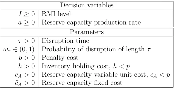
parameters is given in Table 1. Proposition 1 characterizes the optimal risk
Decision variables
I ≥0 RMI level
a≥0 Reserve capacity production rate
Parameters
τ >0 Disruption time
ωτ ∈(0,1) Probability of disruption of lengthτ
p >0 Penalty cost
h >0 Inventory holding cost,h < p
cA>0 Reserve capacity variable unit cost, cA< p ˆ
[image:10.612.158.455.106.257.2]cA>0 Reserve capacity fixed cost
Table 1: Decision variables and parameters of the model
Proposition 1. The optimal RMI I∗ and reserve capacity production rate a∗
are as follows:
I: Inventory strategy: If cˆA≥∆1 and p >
ˆ
h
ωτ, then
I∗ =F−1
τ
ωτp−ˆh
(p+h)ωτ
and a∗ = 0.
II: Mixed strategy: If ∆1 >cˆA>∆2, then
I∗ =Fτ−11− hτ−ˆcA
(h+cA)ωττ
and a∗ = F
−1
τ 1−
ˆ
cA
(p−cA)ωτ τ
−I∗
τ .
III: Process flexibility strategy: If cˆA≤∆2 and (p−cA)ωττ >cˆA, then
a∗ = 1τF−1
τ 1−
ˆ
cA
(p−cA)ωττ
and I∗ = 0,
IV: Passive acceptance: If p≤ ˆh
ωτ and {cˆA≥∆1 or ˆcA ≤∆2}, then
I∗ = 0 and a∗ = 0,
All proofs are provided in the appendix. If the reserve capacity fixed cost
ˆ
cAexceeds the threshold ∆1, the inventory strategy (I) is preferable (for
suffi-ciently large penalty costs) because the reserve capacity is too expensive. The
threshold depends on various model parameters, including RMI holding cost
and reserve capacity variable unit cost. If the reserve capacity fixed cost ˆcA is
below the threshold ∆2 (and the fixed cost for the reserve capacity is not too
high), reserve capacity strategy (III) is preferred, since RMI is becoming too
expensive compared to sourcing from the reserve capacity. In between these
two cases, the mixed strategy (II) is optimal. Otherwise, a passive acceptance
of supply chain disruption risk is optimal (IV).
The threshold ∆1 can be interpreted as the effective penalty costs (e.g.,
penalty costs reduced by the actual reserve capacity production costs) that
are gauged from the relative holding costs to total penalty and holding costs.
The threshold ∆2 can be interpreted as the expected effective inventory
hold-ing costs (e.g., the expected inventory holdhold-ing costs reduced by the expected
reserve capacity production costs). The dependence of ∆1 and ∆2 onh,cˆAand
cA as key parameters is presented in Figures 1 and 2 (withτ = 10, ωτ = 0.05
andp= 40). Sections I, II, and III indicate the areas where inventory strategy,
mixed strategy or reserve capacity strategy, respectively, are optimal. Clearly,
for holding costshand reserve capacity fixed costs ˆcAthat are too high (upper
right-hand corner of the graphs), a passive acceptance of the risk is optimal
(I∗ = 0 anda∗ = 0).
According to Proposition 1, for the inventory strategy, optimal RMI levels
0 0.5 1 1.5 2 2.5 3 3.5 0 2 4 6 8 10 12 14 16 18 20
RMI holding costh
R es er v e ca p a ci ty fi x ed co st ˆ
cA ∆1
∆2
IV
II
[image:12.612.113.492.115.254.2]III I
Figure 1: Phase space for the thresholds ∆1,
∆2 andcA= 15
0 0.5 1 1.5 2 2.5 3 3.5 0 2 4 6 8 10 12 14 16 18 20
RMI holding costh
R es er v e ca p a ci ty fi x ed co st ˆ
cA ∆1
∆2 IV
III II
I
Figure 2: Phase space for the thresholds ∆1,
∆2 andcA= 20
ωτ. For the mixed strategy, the optimal RMI level depends on the expected
additional cost of production through the reserve capacity (ωτcA−ˆh) as well
as the reserve capacity reservation cost ˆcA. The lower this expected additional
cost and the cheaper the reservation cost for the reserve capacity, the lower the
optimal RMII∗and vice versa. The firm’s optimal reserve capacity production
ratea∗ depends on the lost profit (e.g., the difference between penalty cost and
production cost (p−cA)) as well as the reserve capacity reservation cost ˆcA.
The smaller the lost profit and the cheaper the reservation cost for the reserve
capacity, the larger the optimal reserve capacity production rate a∗.
Regarding a sensitivity analysis, the following lemma holds:
Lemma 1. Let the mixed strategy be optimal. Then: 1)I∗ is constant inpand
a∗ increases with p, 2)a∗ decreases withτ for sufficiently largeτ ifhˆ−ωcA≤0
andp > ˆcA+cAωττ
ωττ , 3) ∃ωτ, > ω 0
τ = τ h−ˆcA
τ h+cA such thata
∗
decreases withωτ on the
interval (ωτ0, ωτ,) if ˆcA< τ h.
find:
Lemma 2. Let the mixed strategy be optimal and let demand follow a
nor-mal distribution Fτ( · ). Then: 1) I∗ decreases (increases) with CV if h >
cAωττ+2ˆcA
τ(2−ωτ) (h <
cAωττ+2ˆcA
τ(2−ωτ) ), 2) a
∗ increases with the coefficient of variation of
demand CV.
In other words, it is best to deal with increasing demand volatility by
building up more reserve capacity and by holding more RMI as long as
inven-tory holding costs are not too high. If inveninven-tory holding costs are high, it is
best to deal with increasing demand volatility by holding less RMI. Further
managerial insights based on these findings are discussed in the subsequent
section.
4. Managerial Insights
A manager is typically concerned with two main questions: First, which
risk mitigation strategy is optimal for which products? Second, what are
optimal RMI and/or reserve capacity levels?
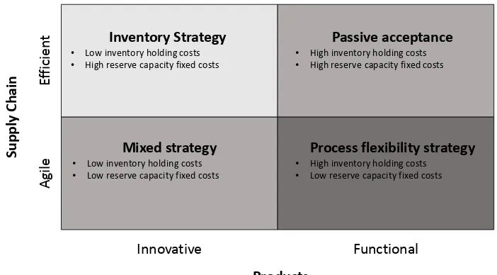
To address the first question, we refer to the typology in Figure 3, where
we identify high (low) inventory holding costs with functional (innovative)
products and high (low) fixed cost for the reserve capacity with an efficient
(agile) supply chain. In the automotive industry, for example, profit margins
are generally low, so the inventory holding costs are relatively high compared to
the total revenue generated. The industry is also capital intensive, resulting
in high fixed costs for the reserved capacity. Therefore, automotive supply
the passive acceptance of supply chain disruption risks is optimal, given the
high inventory holding costs and efficient supply chains. In contrast, for the
innovative pharmaceutical segment of the drug manufacturer Pfizer, the 2015
annual report lists an average cost of sales of 11.2% of revenues (http://
www.pfizer.com/investors). Clearly, for such innovative products, either
an inventory strategy, or a mixed strategy is optimal, depending on the agility
of the supply chain.
Another way to analyze Figure 3 is to identifying the y-axis with demand
uncertainty. An agile [efficient] supply chain corresponds in this scenario to
high [low] demand uncertainty. Our risk mitigation classification matrix can
then be seen as an extension of the classical push-pull process to supply chain
disruption risk where- depending on the product’s characteristic we have to
decide for the right risk mitigation strategy, besides the push-pull boundary
(Simchi-Levi et al., 2004).
To address the second question, we provide structural insights on optimal
RMI and reserve capacity levels. From Lemma 1 and 2 we find the following
main insights:
• The optimal RMI level is constant in the penalty cost.
• The optimal production rate of the reserve capacity may decrease with
the disruption probability.
• While the optimal production rate of the reserve capacity always
in-creases with the coefficient of variation for normally distributed demand,
Products
Innovative Functional
Suppl
y C
ha
in
Ag
ile
Eff
ic
ie
nt • Low inventory holding costsInventory Strategy
• High reserve capacity fixed costs
Mixed strategy
• Low inventory holding costs • Low reserve capacity fixed costs
Passive acceptance
• High inventory holding costs • High reserve capacity fixed costs
Process flexibility strategy
[image:15.612.122.473.119.313.2]• High inventory holding costs • Low reserve capacity fixed costs
Figure 3: Four risk mitigation strategies
variation.
In the following we discuss each insight in detail.
The optimal RMI level is constant in the penalty cost.
This insight is interesting as one might expect that the RMI level increases
with the penalty cost. However, keeping in mind that we apply a mixed
strategy, we observe that only the production rate of the reserve capacity
increases with the penalty cost, and the RMI level remains constant. Once a
certain threshold for the penalty cost is passed, building up reserve capacity
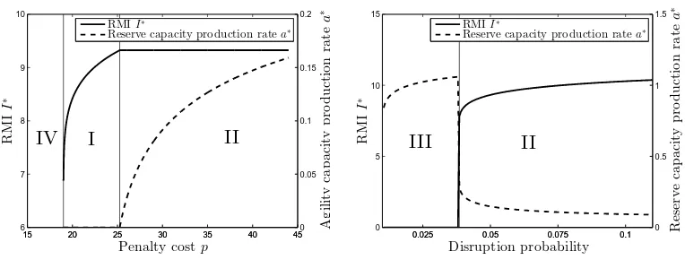
becomes more cost-efficient than building up RMI. We illustrate this insight in
Figure 4, where we show the impact of the penalty cost on RMII∗ and reserve
capacity production rate a∗. The solid curve represents RMI I∗ (levels are
given on the left y-axis) and the dashed curve represents the reserve capacity
graph in two sections. Section I shows the inventory strategy with ˆcA ≥ ∆1.
Section II shows the mixed strategy with ∆1 > cˆA > ∆2. The inventory
strategy (I) is optimal in the approximate range 19 < p < 25, where I∗
increases with p. For p > 25 we pass the breaking point and I∗ remains
constant while a∗ increases with p (mixed strategy II). This plot and the
following ones are based on the following parameters: p= 40, cA = 20, cˆA=
2, τ = 10, ωτ = 0.05 and a normally distributed demand with µ = 1 and
σ = 0.3. In this context, it is important to discuss when the transition from
the inventory strategy to the mixed strategy occurs. From Proposition 1 we
read that the longer the disruption, the more likely the disruption, or the
cheaper the reserve capacity the more likely it is to transit from strategy I to
II.
15 20 25 30 35 40 45
6 7 8 9 10
Penalty costp
R
M
I
I
∗
15 20 25 30 35 40 450 0.05 0.1 0.15 0.2 Ag il it y ca p a ci ty p ro d u ct io n ra te a ∗
RMII∗
Reserve capacity production ratea∗
[image:16.612.120.502.398.543.2]IV I II
Figure 4: Penalty costp
0.025 0.05 0.075 0.1 0 5 10 15 Disruption probability R M I I ∗
0.025 0.05 0.075 0.1 0 0.5 1 1.5 R es er v e ca p a ci ty p ro d u ct io n ra te a ∗ RMII∗
Reserve capacity production ratea∗
II III
Figure 5: Probability of disruptionωτ
The optimal production rate of the reserve capacity may decrease
with the disruption probability.
This insight states that RMI and reserve capacity do not necessarily both
mitigated with reserve capacity only (under some mild assumptions). As the
disruption probability increases, RMI becomes an efficient mitigation lever
and the increase in RMI may cause a decrease in reserve capacity. Figure 5
shows how I∗ and a∗ depend on the disruption probability ωτ. Clearly, for
low disruption probabilities (ωτ <0.04), reserve capacity is the preferred risk
mitigation strategy (section III). The expected overage costs of RMI are too
high compared to the reserve capacity costs. Forωτ >0.04, the mixed strategy
is preferred and we observe that a∗ decreases with ωτ while I∗ increases with
ωτ. This result may be interpreted such that it is not cost effective to keep
inventory and be exposed to high excess inventory charges when disruptions
are rare. Instead, reserving capacity is more cost effective than building up
RMI if disruptions are less likely.
Let us shortly discuss this insight in the context of the pharmaceutical
company. For the pharmaceutical supply chain upstream sites that may
in-volve complex biological manufacturing processes are more likely to be
dis-rupted than downstream sites that rather focus on simple packaging
proce-dures. Thus, the higher disruption probability at the upstream sites may
induce the firm to hold less RMI and more reserve capacity upstream, whereas
the downstream sites with the lower disruption probability are better-off with
While the optimal production rate of the reserve capacity always
increases with the coefficient of variation for normally distributed
demand, the optimal RMI level may decrease or increase with the
coefficient of variation.
This insight reveals a key difference between RMI and reserve capacity. As
RMI is decided prior to the occurrence of a disruption, there is the risk of
incurring overrage costs (inventory holding costs) or underage coasts (penalty
costs). Clearly, if inventory holding costs are high [low], it is optimal to hold
less [more] RMI as demand uncertainty increases (compare discussion of the
newsvendor problem). RMI is an on-going decision that can be adapted to the
demand uncertainty of the product (for example due to life-cycle changes). In
contrast reserve capacity is a design decision that is likewise decided prior to
the occurrence of a disruption. However, the production rate that is used in
the event of a disruption can be adapted after the occurrence of the disruption.
Thus, there is no additional overrage cost in the event of a disruption. Thus,
the reserve capacity increases as demand uncertainty increases.
In Figure 6 we show how I∗ and a∗ depend on the disruption time τ. As
expected, RMI increases with the disruption time τ. In contrast, the reserve
capacity shows a non-trivial result. For 4 < τ ≤ 15, a∗ and I∗ increase with
τ. Both risk mitigation levers are complements. Forτ >15, a∗ decreases with
τ whereas I∗ increases with τ. The decrease of a∗ can be explained by the
0 10 20 30 40 50 60 0
50 100
Disruption timeτ
R
M
I
I
∗
0 10 20 30 40 50 600
0.1 0.2
R
es
er
v
e
ca
p
a
ci
ty
p
ro
d
u
ct
io
n
ra
te
a
∗
RMII∗
Reserve capacity production ratea∗
[image:19.612.216.404.113.258.2]I II
Figure 6: Disruption timeτ
5. Conclusion and Outlook
We have examined optimal RMI and reserve capacity decisions under
sup-ply chain disruption risk and stochastic demand. We quantify four main risk
mitigation strategies: inventory, mixed and reserve capacity strategy, and
de-rive structural insights. We illustrate how the optimal risk mitigation strategy
depends on product characteristics (innovative vs functional) and supply chain
characteristics (agile versus efficient).
A main limitations of our modeling framework is the assumption of a zero
lead time. Clearly, this assumptions allow us to focus the analysis entirely on
the role of disruptions risk when determining optimal RMI and reserve capacity
quantities. However, by doing so, we neglect potential synergies between safety
inventory, which is neglected due to zero lead time, and RMI.
As an avenue for future research we suggest to expand this framework
to include multi-echelon supply chains with product transformation at each
echelon. Given that various factors push RMI and reserve capacity up- and
Appendix A. Proof of Proposition 1
Proof. The firm minimizes the expected loss L(I, a) by determining the
opti-mal RMI I and reserve capacity production rate a, which are non-negative:
min
I≥0,a≥0 L(I, a)
=ωτ p
Z ∞
I+aτ
x−I −aτfτ(x)dx
+h
Z I
0
(I−x)fτ(x)dx+cA
Z I+aτ I
(x−I)fτ(x)dx
+cAaτ
1−Fτ I+aτ
!
+ 1−ωτ
hI + ˆcAa. (A.1)
We introduce the Lagrangian multipliers λI and λA to satisfy the constraints
I ≥0 and a≥0. The Karush-Kuhn-Tucker condition leads to four cases:
• I = 0, a ≥0 with λI ≥0, λa = 0 (Process flexibility strategy)
• I ≥0, a≥0 withλI = 0, λa = 0 (Mixed strategy)
• I ≥0, a= 0 with λI = 0, λa≥0 (Inventory strategy)
• I = 0, a = 0 with λI ≥0, λa≥0 (Passive acceptance of risk)
For the mixed strategy we find:
0 = ∂L(I, a)
∂I = ˆh−λI+ωτ
−p+Fτ I+aτ
(p−cA) +Fτ(I)(h+cA)
where ˆh= 1−ωτ
h, and
0 = ∂L(I, a, τ)
∂a (A.3)
= ˆcA−λA+ωτ
cAτ−pτ +Fτ I+aτ
(p−cA)τ
.
Both solutions are unique. We have:
Fτ(I+aτ) =
ωτ(p−cA)τ−cˆA
ωτ(p−cA)τ
(A.4)
and
Fτ(I) =
ωτ[p−Fτ(I+aτ)(p−cA)]−ˆh
ωτ(h+cA)
, (A.5)
which leads to
Fτ(I) =
(ωτcA−ˆh)τ + ˆcA
ωττ(h+cA)
. (A.6)
For the inventory strategy we note that a= 0 for ˆcA ≥∆1. We find from Eq.
(A.2):
Fτ(I) =
ωτp−ˆh (p+h)ωτ
. (A.7)
For reserve capacity we note that I = 0 for ˆcA≤∆2. We find from Eq. (A.4):
Fτ(aτ) =
ωτ(p−cA)τ −ˆcA
ωτ(p−cA)τ
. (A.8)
Second-order condition: We calculate the matrix elements of the corresponding
Hessian matrix: ∂I∂a∂2L =ωττ(p−cA)fτ(I+aτ), ∂
2L
∂I2 =ωτ(p−cA)fτ(I+aτ) + (h+cA)fτ(I), and ∂
2L
Hessian is given by:
|H| = ω2(τ)
(p−cA)fτ(I+aτ) + (h+cA)fτ(I) τ(p−cA)fτ(I+aτ)
τ(p−cA)fτ(I+aτ) τ2(p−cA)fτ(I+aτ)
= ω2(τ)τ2(p−cA)fτ(I+aτ)
(p−cA)fτ(I+aτ) + (h+cA)fτ(I) 1
(p−cA)fτ(I+aτ) 1
= ω2(τ)τ2(p−cA)(h+cA)fτ(I+aτ)fτ(I)
≥ 0. (A.9)
Appendix B. Proof of Lemma 1
Proof. It is sufficient to look at the following sensitivities: Sensitivity of I∗
with h:
d dh
1− hτ −ˆcA
(h+cA)ωττ
=− cAωττ
2+ ˆc
A
(h+cA)ωττ
2 <0.
Sensitivity ofI∗ with ωτ:
d dωτ
1− hτ−cˆA
(h+cA)ωττ
= hτ −ˆcA
(h+cA)τ ω2τ
.
This term is greater than zero because ˆcA < ∆1 = τ
hp+ph − hcA
p+h
≤ τ h for
the mixed strategy. Sensitivity of I∗ with cA:
d dcA
1− hτ−cˆA
(h+cA)ωττ
= hτ −ˆcA
(h+cA)ωττ
ωττ =
hτ −ˆcA (h+cA)
Sensitivity ofa∗ with cA:
d dcA
1− ˆcA
(p−cA)ωττ
=− cˆA
(p−cA)ωττ
2ωττ =−
ˆ
cA
(p−cA)
2
ωττ
<0.(B.2)
Sensitivity ofa∗ with p:
d dp 1−
ˆ
cA (p−cA)ωττ
= ˆcA
(p−cA)ωττ
2ωττ =
ˆ
cA (p−cA)2ωττ
>0. (B.3)
Regarding the sensitivity of a∗ with ωτ, we assume that ˆcA < τ h. For
ωτ =ωτ0 = τ h−ˆcA
τ h+cA we have a ∗
0 >0 andI
∗
= 0 (risk mitigation strategy III). For
ωτ > ωτ0 we havea
∗
0 >0 and I
∗ >0, and dI∗
dωτ >0 (risk mitigation strategy II).
Therefore,∀ >0 ∃ωτ =ωτ,> ωτ0 : I
∗(ω
τ =ωτ,) = . Then:
d(I∗+a∗τ)
dωτ
|ωτ=ωτ, =
ˆ
cA
fτ(I∗+a∗τ)(p−cA)ω2ττ
|ωτ=ωτ, =
ˆ
cA
fτ(+a∗τ)(p−cA)ωτ,2 τ
=K.
(B.4)
and
dI∗ dωτ
|ωτ=ωτ, =
hτ −cˆA
fτ(I∗)(h+cA)τ ω2τ
|ωτ=ωτ, =
hτ −ˆcA
fτ()(h+cA)τ ω2τ,
=K0
Since fτ(x) is a smooth and positive functions for x > 0 with fτ(0) = 0, we
can choose a ωτ, > ωτ0 such that K < K
0 and therefore d(I∗+a∗τ)
dωτ |ωτ=ωτ, <
dI∗
dωτ|ωτ=ωτ,. Therefore
da∗
dωτ <0 on the interval (ω 0
τ, ω
0
Appendix C. Proof of Lemma 2
Proof. If the demand distribution is given by a normal distribution N(µ, σ),
we have:
I∗ =F−1(β) = µ+σ√2 erf−1(2β−1) (C.1)
withβ = (ωτcA−ˆh)τ+ˆcA
(h+cA)ωττ . Using the Maclaurin series for the inverse error function
erf−1, we have:
I∗ =F−1(β) = µ+σ√2
∞
X
k=0
ck 2k+ 1
√ π
2 (2β−1)
2k+1
(C.2)
where c0 = 1 and ck =
Pk−1
m=0
cmck−1−m
(m+1)(2m+1). Since ck ≥ 0 ∀k ∈ {1, ..,∞} we
have thatI∗ increases with CV, if β > 12 and I∗ decreases with CV, if β < 12.
Otherwise, I∗ remains constant.
If the demand distribution is given by a normal distribution N(µ, σ), we
have:
a∗ = 1
τ
F−1(α)−F−1(β)=σ √
2
τ (erf −1
(2α−1)−erf−1(2β−1)) (C.3)
withα = (p−cA)ωττ−ˆcA
(p−cA)ωττ . Using the Maclaurin series for the inverse error function
erf−1, we have:
a∗ =σ √ 2 τ ∞ X k=0 ck 2k+ 1
√ π
2
2k+1
(2α−1)2k+1−(2β−1)2k+1 (C.4)
References
Berger, P.D., A. Gerstenfeld, A.Z. Zeng. 2004. How many suppliers are best?
a decision-analysis approach. Omega 32 9–15.
Bi¸cer, I. 2015. Dual sourcing under heavy-tailed demand: an extreme value
theory approach. International Journal of Production Research 53 (16)
4979–4992.
Bi¸cer, I¸sık, Ralf W Seifert. 2017. Optimal dynamic order scheduling under
capacity constraints given demand-forecast evolution. Production and
Op-erations Management 26 (12) 2266–2286.
Cattani, K., E. Dahan, G. Schmidt. 2008. Tailored capacity: Speculative and
reactive fabrication of fashion goods. International Journal of Production
Economics 114 416–430.
Chopra, S., M.S. Sodhi. 2004. Managing risk to avoid supply-chain breakdown.
MIT Sloan Management Review 46 52–62.
G¨urler, ¨U., M. Parlar. 1997. An inventory problem with two randomly available
suppliers. Operations Research 45 (6) 904–918.
Hendricks, K.B., V.R. Singhal. 2005. An empirical analysis of the effect of
supply chain disruptions on long-run stock price performance and equity
risk of the firm. Production and Operations Management 14 35–52.
Huang, L., J-S. Song, J. Tong. 2016. Supply chain planning for random
de-mand surges: Reactive capacity and safety stock. Manufacturing & Service
Li, J., S. Wang, T.C.E. Cheng. 2010. Competition and cooperation in a
single-retailer two-supplier supply chain with supply disruption.
Interna-tional Journal of Production Economics 124 137–150.
Liberatore, F., M.P. Scaparra, M.S. Daskin. 2012. Optimization methods for
hedging against disruptions with ripple effects in location analysis. Omega
40 (1)21–30.
L¨ucker, F., S. Chopra, R.W. Seifert. 2016. Disruption risk management for
two-echelon supply chains: Early commitment to finished goods. Working
paper, Swiss Federal Institute of Technology EPFL, Lausanne .
L¨ucker, F., R.W. Seifert. 2016. Building up resilience in a pharmaceutical
sup-ply chain through inventory, dual sourcing and agility capacity.Forthcoming
in Omega .
Niknejad, A., D. Petrovic. 2016. A fuzzy dynamic inoperability input–output
model for strategic risk management in global production networks.
Inter-national Journal of Production Economics 179 44–58.
Parlar, M., D. Perry. 1996. Inventory models of future supply uncertainty with
single and multiple suppliers. Naval Research Logistics 43 191–210.
Reimann, M. 2011. Speculative production and anticipative reservation of
reactive capacity by a multi-product newsvendor. European Journal of
Op-erational Research 211 (1)35–46.
Ruiz-Torres, A.J., F. Mahmoodi. 2007. The optimal number of suppliers
Sarkar, S., S. Kumar. 2015. A behavioral experiment on inventory
manage-ment with supply chain disruption. International Journal of Production
Economics 169 169–178.
Schmitt, A.J., S.A. Sun, L.V. Snyder, Z-J.M. Shen. 2015. Centralization versus
decentralization: Risk pooling, risk diversification, and supply uncertainty
in a one-warehouse multiple-retailer system. Omega 52 201–212.
Simchi-Levi, D., W. Schmidt, Y. Wei. 2014. From superstorms to factory fires:
Managing unpredictable supply-chain disruptions.Harvard Business Review
January-February.
Simchi-Levi, D., E. Simchi-Levi, M. Watson. 2004. Tactical Planning for
Rein-venting the Supply Chain. Springer, USA.
Snyder, L.V., Z. Atan, P. Peng, Y. Rong, A.J. Schmitt, B. Sinsoysal. 2012.
Or/ms models for supply chain disruptions: A review. Working Paper URL
http://papers.ssrn.com/sol3/papers.cfm?abstract_id=1689882.
Tomlin, B. 2006. On the value of mitigation and contingency strategies for
managing supply chain disruption risks. Management Science 52 639–657.
WEF. 2013. Building resilience in supply chains. World Economic Forum,
Industry Agenda .
Yu, H., A. Zeng, L. Zhao. 2009. Single or dual sourcing: Decision-making in