A hybrid model based on functional decomposition for vortex shedding simulations

(1)

City, University of London Institutional Repository

Citation

:

Li, Q. (2017). A hybrid model based on functional decomposition for vortex shedding simulations. (Unpublished Doctoral thesis, City, Universtiy of London)

This is the accepted version of the paper.

This version of the publication may differ from the final published

version.

Permanent repository link:

http://openaccess.city.ac.uk/19667/

Link to published version

:

Copyright and reuse:

City Research Online aims to make research

outputs of City, University of London available to a wider audience.

Copyright and Moral Rights remain with the author(s) and/or copyright

holders. URLs from City Research Online may be freely distributed and

linked to.

(2)

1

A HYBRID MODEL BASED ON FUNCTIONAL

DECOMPOSITION FOR VORTEX SHEDDING

SIMULATIONS

By

Qian Li

B. Eng.

Supervisor

Prof. Qingwei Ma

A thesis submitted to

City, University of London

for the degree of

Doctor of Philosophy

School of Mathematics, Computer Science and Engineering

City, University of London

(3)

2

LIST OF FIGURES

Figure 1.1.1 Offshore pipeline near the free surface (Bluewater) ...23

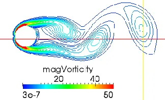
Figure 1.1.2 Illustration of vorticity distribution around a cylinder ...24

Figure 1.1.3 Examples of hybrid numerical models ...26

Figure 1.1.4 Proposed multi-model hybrid approach ...27

Figure 3.3.1 Sketch of the domain size and mesh block configuration ...52

Figure 3.3.2 Lift coefficient variation with three meshes ...54

Figure 3.3.3 Drag coefficient variation with three meshes ...54

Figure 3.3.4 Converged M2 with different Courant numbers ...55

Figure 3.3.5 Distribution of the turbulent viscosity around the cylinder using (a) k-ε model and (b) k-ω SST with Re = 103_...56

Figure 3.3.6 Comparison of mean drag coefficient as the function of Re ...57

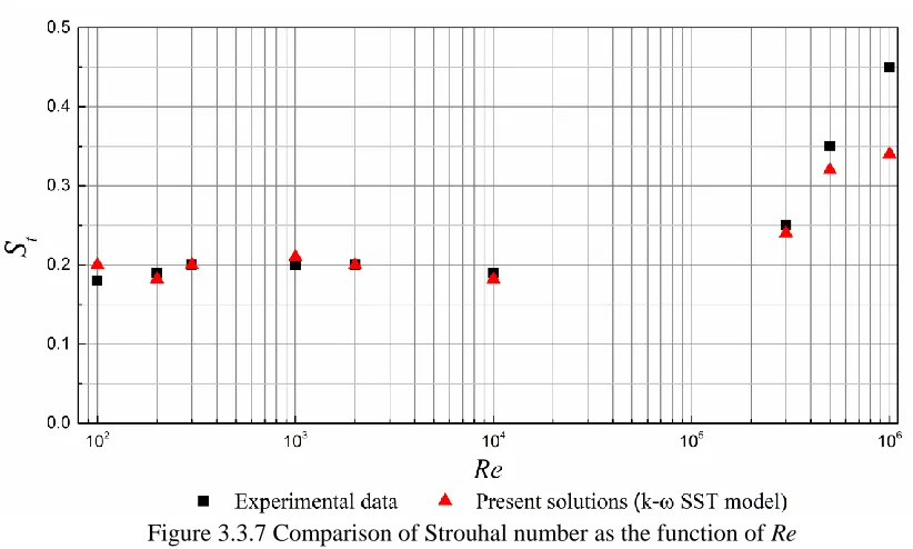
Figure 3.3.7 Comparison of Strouhal number as the function of Re ...57

Figure 3.4.1 Spatial distribution of vorticity and viscosity around the cylinder at Re = 200...60

Figure 3.4.2 Spatial distribution of turbulent viscosity and vorticity around the cylinder at Re = 200 ...60

Figure 3.4.3 Spatial distribution of vorticity and viscosity around the cylinder at Re =106 ...61

Figure 3.4.4 Spatial distribution of turbulent viscosity and vorticity around the cylinder at Re = 106 ...61

Figure 3.4.5 Sketch shows the positions where the profiles are plotted along the transverse and in-line direction ...62

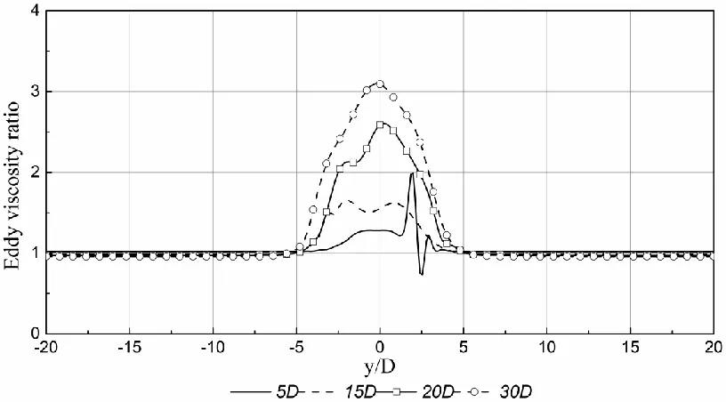
Figure 3.4.6 Turbulent viscosity at Re=1000 along the transverse direction...63

(8)

7

Figure 3.4.8 Turbulent viscosity at Re=1000 along the in-line direction ... 64

Figure 3.4.9 Turbulent viscosity at Re=10000 along the in-line direction ... 64

Figure 3.4.10 Longitudinal distribution of vorticity in the cases of Re=200 and 104_{.. 65}

Figure 3.4.11 Vorticity distribution near moving cylinder at Re=185 for Fr=0.8 ... 66

Figure 3.4.12 Vorticity distribution near moving cylinder at Re=185 for Fr=1.1 ... 66

Figure 3.4.13 Turbulent viscosity from the case of (Re, A/D, Fr) = (185, 0.2, 0.9) along the transverse direction ... 67

Figure 3.4.14 Turbulent viscosity from the case of (Re, A/D, Fr) = (2300, 0.2, 1.1) along the transverse direction ... 67

Figure 3.4.15 Turbulent viscosity distributions of (Re, A/D, Fr) = (2300, 0.5, 0.6) along the transverse direction ... 68

Figure 3.4.16 Turbulent viscosity of (Re, A/D, Fr) = (185, 0.2, 0.9) along the in-line direction... 68

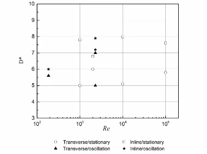
Figure 3.4.19 Range of D* under different working conditions ... 70

Figure 3.5.1 Sketch of the studied multiphase flow problem ... 71

Figure 3.5.2 Working condition matrix for the influential parameters of Froude number and gap ratio ... 72

Figure 3.5.4 Vortex shedding and free surface for different Froude numbers (a) 𝐹𝑟′ = 0.25 (b) 𝐹𝑟′=0.36 at same gap ratio h/D=2. ... 73

Figure 3.5.5 Time history of CL for the h/D=1 with 𝐹𝑟′=0.25 and 𝐹𝑟′=0.36 ... 74

Figure 3.5.6 Vortex shedding and free surface for Froude numbers of 0.25 for a gap ratio of (a) h/D =3; (b) h/D=2; (c) h/D=1; (d) h/D= 0.5 for the Re =100. ... 75

Figure 3.5.7 Time history of CL for the Re=100, 𝐹𝑟′=0.36 with h/D=2.5 and h/D=1 . 76 Figure 3.5.8 Time history of CL for the Re =200 with 𝐹𝑟′=0.25 and 𝐹𝑟′=0.36 ... 76

Figure 3.5.9 Zone 1 and Zone 2 for the tested working conditions ... 77

Figure 4.1.1 Sketch of the hybrid method computational domain ... 81

(9)

8

Figure 4.1.3 Sketch of the viscosity fields mapping order ...86 Figure 4.2.1 Sketch of the boundary conditions for the typical two-phase flow past a circular cylinder ...91 Figure 4.2.2 Sketch of the hybrid method computational domain with the presence of the free surface ...92 Figure 4.2.3 Sketch of the viscosity fields mapping order for the multiphase solver ...95 Figure 5.2.1 Flow chart of the hybrid model algorithm ...99 Figure 5.3.1 Flow chart for the two-phase hybrid solver algorithm ...101 Figure 5.4.1 The face f whose owner is P and neighbour N ...104 Figure 6.1.1 Sketch of two meshes ( • denotes the cell centre of the truncated

overlapping domain mesh; × denotes the cell centre of the quasi-turbulent domain with a coarser mesh) ...111 Figure 6.1.2 Sketch of the block mesh configuration for both the quasi-turbulent and the overlapping domains ...112 Figure 6.1.3 Sketch of the vortex shedding simulation whole procedure using the hybrid method...114 Figure 6.1.4 Time histories of drag and lift coefficients at Re=185 with A/D =0.2 and

𝐹𝑟=0.9 ...115 Figure 6.1.5 Comparison of CD and CLrms between the hybrid model and original RANS

solver for A/D=0.2 ...117 Figure 6.1.6 Comparison of CD and CLrms between the hybrid model and original RANS

solver for A/D=0.4 ...117 Figure 6.1.7 Time histories of drag coefficients with 𝐹𝑟=1.1 and A/D=0.2 at Re=1000 ...118 Figure 6.1.8 Time histories of lift coefficients with 𝐹𝑟=1.1 and A/D=0.2 at Re=1000 ...118 Figure 6.1.9 Comparison of CD as a function of 𝐹𝑟 ...120

Figure 6.1.10 Comparison of CLrms as a function of 𝐹𝑟 ...120

Figure 6.1.11 Power spectra of CL for: (a) 𝐹𝑟=0.8, (b) 𝐹𝑟=0.9, (c) 𝐹𝑟=1.0, (d) 𝐹𝑟=1.1,

(10)

9

Figure 6.1.12 Instantaneous vorticity contours in one period (from (a) to (d)) for cases at low-frequency stage with a 2S mode; (e) time history of lift and drag coefficient for

the same case ... 124

Figure 6.1.13 Instantaneous vorticity contours in one period (from (a) to (d)) for cases at high-frequency stage with a 2P mode; (e) time history of lift and drag coefficient for the same case ... 125

Figure 6.2.1 Configuration of the numerical wave tank ... 126

Figure 6.2.2 Comparison of the wave surface elevation profiles ... 128

Figure 6.2.3 Free surface time history at (x-xc)/𝜆 = -0.4 ... 128

Figure 6.2.4 Free surface time history at (x-xc)/𝜆 =0.055 ... 129

Figure 6.2.5 Free surface time history at (x-xc)/λ =0.4052 ... 129

Figure 6.2.6 Free surface time history at (x-xc)/𝜆 =1.006 ... 129

Figure 7.1.1 CPU time saving against the Reynolds number for the studies cases ... 135

Figure 7.2.1 Streamlines of velocity in the multiphase flow with the dashed line representing the free surface ... 137

Figure 7.2.2 Streamlines of velocity in the single-phase flow with Re=1000 ... 137

Figure 8.2.1 Sketch of the hybrid model deals with different flow properties with different models ... 141

(11)

10

LIST OF TABLES

Table 2.1.1 A summary of the experimental studies for VIV problems ...33

Table 2.2.1 Comparisons of RANS, LES and DNS models in VIV simulation ...36

Table 2.2.2 Numerical simulation of flow past circular cylinder considering the free surface ...38

Table 2.2.3 Comparison of two decomposition approaches ...42

Table 3.3.1 Meshes and Courant number tested ...53

Table 4.2.1 Boundary condition configuration ...91

Table 6.1.1 Disparity between the two solvers under Re=1000 ...114

Table 6.1.2 Disparity between the two solvers under Re=10000 ...114

Table 6.1.3 Comparison between the hybrid model and original RANS solver for the case (Re, A/D, Fr) = (185, 0.2, 1.2) ...116

Table 6.1.6 Comparison between the hybrid model and original RANS solver for the case (Re, A/D, Fr) = (2300, 0.2, 08) ...119

Table 6.2.1 Wave parameters...127

Table 6.2.2 Mesh generation configuration ...127

Table 7.1.1 Comparison of efficiency between the original RANS solver and hybrid model with a stationary cylinder ...133

(12)

11

Table 7.2.1 Comparison of efficiency between the original RANS solve and multiphase hybrid solver ... 138

(13)

12

ACKNOWLEDGEMENTS

I would like to express my sincere gratitude to my supervisor Prof. Qingwei Ma, for his continuous support and guidance. His keen enthusiasm for research always inspire me and encourage me. I really appreciate the knowledge and the insight he has shared with me in our weekly meeting.

Many thanks go to my second supervisor Dr. Shiqiang Yan. I appreciate the patient and generous help he gives me every time I stuck in my research. His high standard requirement and hard-working attitude towards work inspired me a lot as a researcher. Prof. Qingwei Ma and Dr.Shiqiang Yan, they both have taught me so much, and set a good example for my career and life.

Furthermore, the accomplish of this thesis has benefited from the valuable comments given by Prof. Qingwei Ma, Dr. Shiqiang Yan and Dr. Jinghua Wang.

Special thanks to the members of our research group with who I have spent an unforgettable time together and friends in the department have helped me along the way. I am very thankful for the guidance comes from Prof. Weiping Huang and Prof. Lin Zhao. Thanks for their support and encouragement at the Ocean University of China throughout my master study.

I appreciate the sponsorship provided by China Scholarship Council. Also, thanks for the scholarship from Prof. Qingwei Ma and Dr. Shiqiang Yan during my study.

(14)

13

DECLARATION

No portion of the work referred in the thesis has been submitted in support of an application for other degree or qualification of this or any other university or other institute of learning.

I grant powers of discretion to the City, University of London’s Library to allow this thesis to be copied in whole or in part without any reference to me. This permission covers only single copies made for study purpose subject to the normal condition of acknowledgement.

(15)

14

ABSTRACT

Vortex-Induced Vibration (VIV) is one of the significant physics that encounter in the engineering practice. The good understanding of the structure response and technologies to suppress the significant vibration and undesirable forces induced by VIV is of vital importance for the entire design/planning procedure. However, for both the single-phase and multiphase flow, the main challenge is how to significantly improve the simulation efficiency and meanwhile maintain the accuracy.

This research aims to develop a hybrid model which can simulate VIV significantly more efficiently. A novel framework for a hybrid model which is based on the functional decomposition is proposed. The theoretical hypothesis of the hybrid model is that the viscous effect is only significant near the offshore structures or breaking waves, and may be ignored in other areas. In this model, all physical variables are split into two parts. One part is solved by a quasi-turbulent model in whole domain and the other part solved by using a residual turbulent model in a smaller domain. The two models are implemented simultaneously based on their respective meshes and time steps. Due to this feature, the techniques such as the sub-cycle strategy are employed for the improvement of the efficiency without the deterioration of the accuracy.

(16)

15

(17)

16

LIST OF SYMBOLS AND

TECHNICAL TERMS

𝐴 Oscillation amplitude 𝐴/𝐷 Amplitude ratio

𝐷 Cylinder diameter 𝐺 Spatial filter

𝑁 Number of members of the ensemble

𝑇 Wave period

𝑈 Free stream flow velocity

𝐶_𝐷

̅̅̅̅ Mean drag coefficient

𝐶_{𝐿 𝑟𝑚𝑠} Root mean square lift coefficient 𝐶𝐿, 𝐶𝐷 Drag and lift coefficients

𝐶_𝐿𝐴 Amplitude of the fluctuating lift coefficient

𝐶_𝜇 𝐶_𝜇 = 0.09, constant in the k-ε turbulent model

𝐷_𝑐 Crossflow direction domain size 𝐷𝑖𝑛 Distance between inlet and cylinder

𝐷_𝑜𝑢𝑡 Cylinder to outlet distance 𝐹𝐿, 𝐹𝐷 Fluid drag and lift force

𝐹_𝑇 Transition frequency

𝐹_𝑟 Frequency ratio 𝐹𝑟′ Froude number

𝑁𝑐 Critical sub-cycle number

(18)

17

𝑁_𝑡 Total number of independent samples 𝑅𝑒 Reynolds number (𝑈𝐷 𝑣⁄ )

𝑆_𝑡 Strouhal number

𝑈̅ Assemble average velocity of the flow

𝑈_𝑚𝑎𝑥 Maximum velocity magnitude estimated by quasi-turbulent

model

𝑈_𝑚𝑎𝑥∗ Maximum velocity magnitude estimated by the residual model 𝑈𝑟 Reduced velocity

𝑊_𝐶 Critical width of the significant turbulent viscosity zone

𝑓_𝑛 Fundamental natural frequency 𝑓𝑜 Exciting frequency

𝑓_𝑠 Vortex-shedding frequency

𝑚∗ Fluid added masses

𝑢∗_,_𝑝∗ _{Velocity and pressure of the residual field}

𝑢_𝑇, 𝑝_𝑇 Velocity and pressure of the total field

𝑢_𝑛𝑖(𝑥_𝑖, 𝑡) 𝑢(𝑥𝑖, 𝑡) at the nth series

𝑢𝑝𝑖 Potential component of the total velocity in the complementary

RANS equations

𝑦+ Distance from the wall measured in viscous lengths 𝑦_𝑤 Distance from the centre of the first cell to the wall

d Water depth

h Distance from the cylinder to the free surface

h/D Submerged depth

c Coupling boundary in the hybrid method

R Overlapping sub-domain

𝜏_𝑖𝑗𝐿𝐸𝑆 Shear stress term in LES

𝑇 Quasi-turbulent solver domain

_𝑇1 Same domain size to R but different solver is implemented

𝑢𝑖′𝑢𝑗′

̅̅̅̅̅̅ Reynolds stresses

(19)

18

𝑎𝑖𝑗 Deviatoric part of the Reynolds stresses

𝑐α Interface compression coefficient

𝑢_𝑏𝑖 Velocity with which the integration boundary (𝑟) moves.

𝑢_𝑖′(𝑥_𝑖, 𝑡) Fluctuation of the time-averaged value 𝑢_𝜏 Friction velocity

𝛿𝜈 Viscous length scale

𝜇_𝑎𝑖𝑟, 𝜇_𝑤 Dynamic viscosity of air and water

𝜇𝑒𝑓𝑓(𝑥𝑖, 𝑡) Effective dynamic viscosity

𝜈𝑇(𝑥𝑖, 𝑡) Turbulent /eddy viscosity

𝜈_𝑒𝑓𝑓(𝑥𝑖, 𝑡) Effective kinematic viscosity

𝜌_{𝑎𝑖𝑟,} 𝜌_𝑤 Densities of air and water

𝜏_𝑤 Wall shear stress

𝜑_{𝑙𝑖𝑓𝑡} Lift angle

∆𝐿 Minimum mesh size in the quasi-turbulent domain ∆𝑇1 Time step for the quasi-turbulent field

∆𝑇2 Time step for the residual solver

∆𝑙 Minimum mesh size in the residual field domain α Volume fraction

γ Diffusion coefficient

Δ𝑓 Filter width

σ Surface tension coefficient

к Local interfacial curvature 𝑘 Turbulent kinetic energy 𝛷 Velocity potential

𝛻1 𝑓

Surface gradient operator

𝛿 Boundary-layer thickness 𝜀 Turbulent dissipation

(20)

19

𝜆 Wavelength

𝜇 Dynamic viscosity

𝜇′(𝑥_𝑖, 𝑡) Effective dynamic viscosity of the quasi-turbulent field

𝜈 Constant molecular viscosity

𝜈′(𝑥𝑖, 𝑡) Effective kinematic viscosity of the quasi-turbulent field

𝜌 Flow density

𝜔 Specific turbulent dissipation rate

Abbreviation

2G-URANS Second-Generation URANS ALE Arbitrary Lagrangian–Eulerian DES Detached Eddy Simulation DNS Direct Numerical Simulation DOF Degree of freedom

FEM Finite Element Method FFT Fast Fourier Transform

FNPT Fully Nonlinear Potential Theory FSI Fluid-Structure Interaction FVM Finite Volume Method

HOS Higher-Order Spectrum method HPC High-Performance Computing

HR High Reynolds number wall treatment

IMLPG_R Improved Meshless Local Petrov Galerkin method with Rankine source solution

KC Keulegan Carpenter number LES Large Eddy Simulations

LR Low Reynolds number wall treatment MLPG Meshless Local Petrov Galerki

MPS Moving Particle Semi-implicit

(21)

20 2P Two vortex pairs each cycle PANS Partially Filtered Navier-Stokes

PISO Pressure Implicit with Splitting of Operators QALE Quasi-Arbitrary-Lagrangian-Eulerian

QDNS Quasi-Direct Numerical Simulation

RANS Reynolds-Averaged Navier–Stokes equations RKE Realizable k-ω turbulent model

RMS Root mean square

2S Two single vortices shed each cycle S-A Spalart–Allmaras turbulent model SGS Sub Grid Scale

SPH Smoothed Particle Hydrodynamics SST Shear-Stress-Transport model

SWENSE Spectral Wave Explicit Navier-Stokes Equations approach URANS Unsteady Reynolds-averaged Navier–Stokes equations

VEM Vortex Element Methods VIV Vortex Induced Vibration VLES Very-Large Eddy Simulation

(22)

21

1

INTRODUCTION

1.1 Background

(23)

22

damage, the issues associated with VIV must be carefully addressed during the entire design/planning procedure, such as towing, installation, operation and demolishment. For this purpose, understanding of the structure response and technologies to suppress the significant vibration and undesirable forces induced by VIV become highly demanded.

(24)

23

Figure 1.1.1 Offshore pipeline near the free surface (Bluewater, 2017)

No matter which way is applied, the computational cost for the VIV modelling is often high. In order to achieve reasonable results in an allowable CPU time, most of the numerical simulation of this kind is limited to a small computational domain surrounding the structures (~100D, where D is the characteristic dimension of the structure) and/or in two-dimension. It has also been demonstrated by Pope (2001) that, to capture the evolution of small eddies and to maintain the numerical stability, there are decreases of the spatial scales and temporal scales with the relationship of

𝑅𝑒−34 _and 𝑅𝑒− 1

2 _{respectively with the increase of the Reynolds number. The}

computational cost may be dramatically increases if a free surface flow is involved. In fact, for most of the offshore structures, which are often exposed to water waves, the free surface effect may need to be taken into account, especially, for the pipe segments near the water surface, as illustrated in Figure 1.1.1, and transmission pipelines during loading/offloading operation. Within the NS solver, one need to track or identify the free surface to correctly model the free surface flow and water waves. Classic models include multi-phase NS with volume of fluid technology (short as VOF and proposed by Hirt & Nichols (1981)), single-phase/multi-phase level set methods, multi-phase NS with marker-and-cell approach and single-phase/multi-phase meshless methods (e.g. Smoothed Particle Hydrodynamics (SPH), Moving Particle Semi-implicit method (MPS) and the Meshless Local Petrov Galerkin methods (MLPG)). Not only the extra cares on effectively resolving the free surface and accurately modelling the water wave

FPSO

(25)

24

[image:25.612.208.370.303.402.2]

propagating, another constraint induced by the free surface flow is the size of the computational domain. It may be essential to cover the dimension in the depth direction from the water surface to the seabed, i.e. thousands meters for deep water application; at least 5~10 wave lengths (Wang 2016) in the horizontal plane at a scale of hundreds to thousands meter. Unfortunately, all the above-mentioned methods are too time-consuming for practical applications for such a large computational domain. Thus, simplified and empirical numerical models are widely used in the industrial design practices, with aid of experimental investigation. “Is there any way to accelerate the computing without loss of accuracy?” may be one of the most frequently questions in the numerical practices for VIV, high-Re problems and other problems with significant turbulent effects.

Figure 1.1.2 Illustration of vorticity distribution around a cylinder

One direct way for accelerating the numerical simulation is to conduct highly parallel computing using high-performance computing (HPC). On the other hand, efforts have been devoted to developing more robust modelling strategy or methodologies. The developments in these two directions do not conflict with each other and shall be combined to maximise the computational efficiency. In this work, the latter is focused.

(26)

25

modelling takes effects in the entire computational domain. In fact, the turbulent effects and vortex shedding may only be significant near the structure and in the wake area, as demonstrated by Figure 1.1.2, which shows the vorticity distribution around a fixed cylinder subjected to constraint inflow. Far away from these regions, the flow may be dominated by inertia force, e.g. gravity-driven flow, and the viscous effects may be ignored. In many cases, the potential flow may be sufficient to describe the flow feature in these regions, e.g. the propagation of the waves from far-field towards near field. This fact initiates the development of hybrid approaches, which combining different numerical methods and physical models.

(27)

26

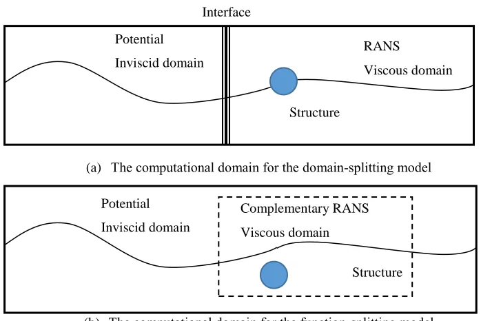
(a) The computational domain for the domain-splitting model

[image:27.612.102.451.93.326.2]

(b) The computational domain for the function-splitting model

Figure 1.1.3 Examples of different hybrid numerical models

By using these strategies, a few hybrid models have been developed. The majority couple (1) potential model and other higher-order potential model (e.g. Wang et al., 2016); (2) potential theory (or other equivalent simplified model, e.g. nonlinear Schrödinger’s equation and Euler’s equation) and NS solver, e.g. RANS with or without

turbulent modelling (e.g. Sriram et al., 2014); (3) incompressible NS solver with compressible NS solver (e.g. Martínez Ferrer et al., 2016); and (4) RANS approach with turbulent model and LES (Fan et al.,2017; Wei et al., 2016; Sajjadi et al., 2017; Kocutar

et al., 2015; Gopalan et al., 2013). Considering the fact that the turbulence modelling is essential near the structure for the problems concerned here, i.e. VIV problems, available hybrid models may only couple the turbulent NS solver with either a potential theory (2) or another turbulent NS solver (4). Option (4) couples two turbulent NS solvers and, therefore, its computational efficiency may be impractical low; whereas Option (2) may suffer from a sudden change of the fluid properties from an inviscid/irrotational flow (no viscosity) to a turbulent flow (constant physical viscosity and unsteady turbulent/eddy viscosity), especially for high-Re problems, and consequently may be either numerically unstable or computationally costly (e.g.

RANS

Viscous domain Potential

Inviscid domain

Interface

Structure

Potential Inviscid domain

Complementary RANS Viscous domain

(28)

27

requires large transitional zone for a smooth transition of viscous effects, large domain for solving turbulent models small time step size and so on).

Figure 1.1.4 Proposed multi-model hybrid approach

This issue can be addressed by replacing the turbulent NS solver in Option (2) by a hybrid model coupling simplified RANS solver (e.g. the RANS without turbulent models) and turbulent NS solver (e.g. the RANS with turbulent model). Overall, one example of the new approach can be illustrated in Figure 1.1.4. The induction of the laminar NS solver (constant physical viscosity) between the inviscid/irrotational flow solver (no viscosity) and the turbulent flow solver (constant physical viscosity and unsteady turbulent/eddy viscosity) makes the viscous effects changes step by step, increasing the numerical instability. For the viscous domain, the solution of the turbulent modelling may only require in a small region near the structure, saving the CPU time on resolving the turbulent/eddy viscosity. To the best of my knowledge, no attempts have been found in the public domain to couple a simplified RANS solver with a turbulent solver.

1.2 Aim and objectives

This research aims to develop a hybrid model coupling a simplified RANS solver with a turbulent RANS solver for effectively modelling VIV. The functional decomposition (velocity decomposition) strategy is adopted. The objectives comprise:

1. Understanding the spatial-temporal distribution of the turbulent/eddy viscosity associated with flow around submerged structures with or without free surface effects, which is the foundation to develope the hybrid model;

RANS

Viscous domain No turbulent viscosity Potential

Inviscid domain

Interface

Structure

(29)

28

2. Developing the hybrid model to couple the simplified RANS and turbulent RANS solvers;

3. Numerically investigating the performance of the developed hybrid model, e.g. the computational efficiency, accuracy and convergence;

4. Investigating the feasibility of coupling the developed hybrid model with a fully nonlinear potential model in a domain-splitting way, as sketched in Figure 1.1.4.

It is noted that only two-dimensional development and investigation will be considered in this thesis. One may apply the developed model to many scenarios, e.g. a long-span horizontal pipeline subjected to a unidirectional wave/current; a strip of the 2D fluid-structure interaction model in the above-mentioned strip method. One may also consider this research as a conceptional study, which proves the superiority of the hybrid model over the conventional model in terms of computational robustness, for the development of 3D hybrid model in the future.

1.3 Outline of the thesis

(30)

29

2

LITERATURE REVIEW

This section of the literature review starts with the classical VIV problem studied by both experimental and numerical approaches regarding both the single- and multi-phase flow. Due to the complexity of the VIV study, the movement of the cylinder is usually classified into two types: the free vibration and the forced vibration. Hence, review of the free and forced vibration will be given separately. After that, the numerical simulation models, both the traditional single models and the hybrid models belonged to different categories are compared and reviewed. At last, discussions are given about the existing problems, and the objective of this study is described.

2.1 Experimental researches

2.1.1 Free and forced vibration studies

(31)

30

Brika & Laneville (1993, 1995), were the first to show evidence of the 2P (P is short for vortex pairs) vortex wake mode from free vibration and confirmed the earlier explanation by Williamson & Roshko (1988) for the hysteresis loop in terms of a change in wake vortex patterns. Brika & Laneville (1993, 1995) found a clear correspondence of the 2S mode with the initial branch of response, and the 2P mode with the lower branch. However, Khalak & Williamson (1997) observed that the phenomena at low mass ratios and low mass damping are distinct from those mentioned above. A direct comparison is made between the response in water by Khalak & Williamson (1997) with the largest-response plot of Feng (1968). The lighter body has a value of mass ratios yielded a much higher peak amplitude. Khalak & Williamson (1997) also observed the existence of three distinct branches, in which the low mass ratio type of response is characterised by not only the initial branch and the lower branch, but also by the new appearance between the other two branches of a much higher upper response branch. Regarding the phenomenon of ‘‘lock-in’’ or synchronization, however, for the low mass ratio in water in the experiment of Khalak & Williamson (1997), the body oscillates at a distinctly higher frequency, is different to the traditional concept in the studies of Blevins (1990) and Sumer & Fredsoe (2006).

(32)

31

these modes from controlled vibration is that they provide a map of regimes, within which we observe certain branches of free vibration. One deduction from the Williamson & Roshko’s (1988) study was that the jump in the phase of the transverse force in Bishop & Hassan’s (1964) classical forced vibration study, and also the jump in phase measured in Feng’s (1968) free vibration experiments, were caused by the changeover of mode from the 2S to the 2P mode. This has since been confirmed in a number of free-vibration studies like Brika & Laneville (1993), etc. Cheng & Moretti (1991) conducted a series of experiments with a circular cylinder subjected to forced transverse vibration in a uniform cross-flow at Reynolds numbers of 1500 and 1650. Blevlns & Burton (1976) have provided extensive data for the amplitude ratio versus the lift coefficient for a variety of conditions. Hover et al. (1997); Hover et al. (1998) and Hover et al. (2001), Gopalkrishnan et al. (1994), developed a novel virtual cable testing apparatus and conducted a series of tests using this faculty. A further significant result has been presented by Bearman et al. (2001), who have presented an excellent agreement between in-line response measurements at Re=104 and Re=105. There was also good agreement for the limited transverse VIV response data at these Reynolds numbers. Sheridan et al. (1998) and Carberry et al.(2001, 2003, 2004, 2005) made extensive measurements of force from controlled vibrations of cylinders, providing a number of interesting results and data can be used for numerical validation.

2.1.2 VIV subject to the free surface

(33)

32

Kármán wake with the amplitude of the fluctuating lift force larger than that for deep water case. The periodic vortex shedding appears to be suppressed and the lift varies little with time in both Modes II and III. The flow over the top of the cylinder remains attached to and separates from the free surface for Modes II and III, respectively. In Mode III, the separated flow forms a jet which can either remain attached to the cylinder or flow downwards obliquely. Saelim (1999) investigated the one-degree-of-freedom (one-DOF) transverse VIV of an elastically mounted rigid horizontal circular cylinder beneath a free surface. The results showed that, for small h/D, very large regions of hysteresis occur in the variation of vibration amplitude as a function of reduced velocity. For large values of h/D, the vibration frequency is higher than natural structure frequency and lower than the vortex shedding frequency in the lock-in zone; for very small h/D, the vibration frequency takes on values close to the vortex shedding frequency, hence much higher than natural structure frequency. Rockwell et al. (2003) later presented some typical vortex shedding regimes for h/D = 0. Cetiner & Rockwell (2001) experimentally investigated the stream wise oscillations under several combinations of amplitude ratio and frequency ratio. They found that the transverse force is phase-locked to the cylinder motion when h/D≈0 and such locked-in states are

destabilised because of an instantaneous jet-like flow mentioned above when h/D is finite. Sheridan et al. (1997) conducted experiments using the PIV technique and found that close to a free surface the near-wake structure falls under a number of modes which are very different from those of the deeply submerged cylinder wake. Carberry (2002) observed three different wake states as gap ratios decreases which also found by other experimental (Sheridan et al., 1997) and numerical (Reichl et al., 2005) studies.

(34)

33

cylinder circumference and integrated it to yield the in-line force. The results were given in terms of drag and inertia coefficients as functions of the KC number and the reduced velocity. Yokoi & Kamemoto (1994a) examined the vortex shedding frequency and pattern of an in-line oscillating circular cylinder in uniform flow at rather small KC

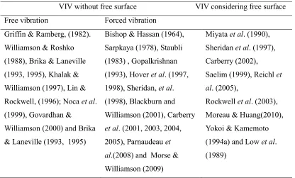
[image:34.612.125.541.274.525.2]

numbers and found that the vortex shedding frequency was synchronised with multiples of the oscillation frequency. The summary of the experimental studies carried out for both free and forced/controlled vibration situation with or without the presence of the free surface are given in Table 2.1.1.

Table 2.1.1 A summary of the experimental studies for VIV problems

VIV without free surface VIV considering free surface Free vibration Forced vibration

Griffin & Ramberg, (1982). Williamson & Roshko (1988), Brika & Laneville (1993, 1995), Khalak & Williamson (1997), Lin & Rockwell, (1996); Noca et al. (1999), Govardhan &

Williamson (2000) and Brika & Laneville (1993, 1995)

Bishop & Hassan (1964), Sarpkaya (1978), Staubli (1983) , Gopalkrishnan (1993), Hover et al. (1997, 1998), Sheridan, et al. (1998), Blackburn and Williamson (2001), Carberry

et al. (2001, 2003, 2004, 2005), Parnaudeau et al.(2008) and Morse & Williamson (2009)

Miyata et al. (1990), Sheridan et al. (1997), Carberry (2002),

Saelim (1999), Reichl et al. (2005),

Rockwell et al. (2003), Moreau & Huang(2010), Yokoi & Kamemoto (1994a) and Low et al. (1989)

2.2 Numerical simulations

2.2.1 Single models

(35)

34

resolve all details. In RANS model, the turbulent flow behaviour is approximated modelled by using the Reynolds-Averaging concept to simplify Navier-Stokes equations. This model provides results for mean quantities with engineering accuracy at moderate cost for a wide range of turbulent flow problems. Therefore, RANS is the most widely used turbulent in the VIV simulations. Guilmineau & Queutey (2004) conducted a simulation adopting the incompressible two-dimensional RANS equations together with a SST k-ω model for a low mass-damping case, where the Reynolds number is in the range 900–15000. The simulations predicted correctly the maximum amplitude. However, fail to match the upper branch found experimentally. Ünal, et al. (2010) investigated four turbulent models: Spalart–Allmaras (S–A), Realizable k-ε (RKE), Wilcox k-ω (WKO) and Shear-Stress-Transport k-ω (SST), and found that both WKO and SST models exhibited successful performance producing highly correlated predictions of the main flow characteristics with the experimental data. In order to provide a reliable and useful assessment tool for the engineering design work, Ong et al. (2009) conducted a simulation covering the supercritical to upper-transition flow regimes around a 2D smooth circular cylinder.

The model of LES is based on a filtering concept (Leonard, 1975). If a spatial filter

𝐺 = 𝐺_𝛥𝑓is applied to a variable 𝜙, this yields a smoothed counterpart 𝜙̅ with scales smaller than the filter width Δ𝑓 being removed. Numerical simulations of VIV using LES are extensive. For instance, Al-Jamal & Dalton (2004) have performed a 2D LES study of the VIV response of a circular cylinder at a Reynolds number of 8000 with a range of damping ratios and natural frequencies. Kim (2014) examined the transition process between two different wake states in the frame of LES for the high Reynolds number flows range from 5500 to 41300. Other simulations include Selvam (1997), Wang & Catalano (2001), Catalano, et al.( 2003) and Breuer (2000).

(36)

35

same order as the viscous stresses, since the typical eddy-viscosity levels are very close to the molecular viscosity. The cost of LES in the entire boundary layer exceeds the computing power by orders of magnitude. As a result, RANS is the only choice for most of the boundary layer. RANS and LES show their advantage in the boundary layer and separation regions, separately. However, regarding the three-dimensional separation, it is beyond the capability of RANS and the LES model is often employed.

DNS is model-free numerical simulations of turbulence. DNS differs from the RANS in that the turbulence is explicitly resolved, rather than modelled by a closure model. It also differs from LES in scales, even the very smallest ones are captured and no need for a subgrid-scale model. Its advantage is the ability to provide complete knowledge, unaffected by approximations within the simulation period (Coleman & Sandberg 2010). This ability, however, comes at a high price and severe limitation on the maximum Reynolds number and complex geometry that can be considered, which prevents DNS from being used as a general-purpose design tool. DNS as a powerful model has been adopted in the VIV simulations as well. Dong & Karniadakis (2005) conducted a DNS simulation for turbulent flows past a stationary circular cylinder and a rigid cylinder undergoing forced harmonic oscillations at Re =10000. Comparisons with the available experimental data show that the simulation has captured the flow physical quantities and the statistics of the cylinder wake correctly. Dong et al. (2006) investigated the effects of Reynolds number (at Re=3900, 4000 and 10000) by combining PIV measurements and DNS simulations. The statistical characteristics of the cylinder wake and on the shear-layer instability in the transitional range are observed altered with the variation of Reynolds number.

Comparing the three models, there are not only differences but similarities. As for RANS modelling, the nonlinear convection term in the transport equation introduces an unclosed term, describing the impact of the sub-filter scales on the resolved motion, it is replaced by a model term 𝜏_𝑖𝑗𝐿𝐸𝑆 in LES. For the efficiency reason, the ratio of the filter width Δ𝑓 to the step size of the grid Δ𝑔 is usually set equal to one or a small integer.

(37)

36

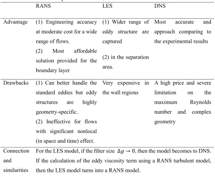
[image:37.612.71.492.177.524.2]

limit Δ𝑔 → 0, the SGS model vanishes so that the simulation turns into a DNS without turbulence model. This structural similarity is also the foundation of the RANS/LES/DNS hybrid method. The comparisons of RANS, LES and DNS models are given in Table 2.2.1.

Table 2.2.1 Comparisons of RANS, LES and DNS models in VIV simulation RANS LES DNS

Advantage (1) Engineering accuracy at moderate cost for a wide range of flows.

(2) Most affordable solution provided for the boundary layer

(1) Wider range of eddy structure are captured

(2) in the separation area.

Most accurate and approach comparing to the experimental results

Drawbacks (1) Can better handle the standard eddies but eddy structures are highly geometry-specific.

(2) Ineffective for flows with significant nonlocal (in space and time) effect.

Very expensive in the wall regions

A high price and severe limitation on the maximum Reynolds number and complex geometry

Connection and

similarities

For the LES model, if the filter size Δ𝑔 → 0, then the model becomes to DNS. If the calculation of the eddy viscosity term using a RANS turbulent model, then the LES model turns into a RANS model.

(38)

37 2.2.2 Single models considering the free surface

Regarding the flow past a circular cylinder, the most studied case is the stationary circular cylinder subject to the inline steady flow. However, fewer considering the influence of the free surface. According to the previous studies, it is generally agreed that the pressure distribution and the near wake structure of the circular cylinder near the free surface are very different to that deeply submerged cylinder situations.

Considering the effect of the submerged depth, Chung (2015) numerically compared the cases of gap ratio= 0.4, 0.8 to deep water situation. The jump of the amplitude and phase of lift was also reported, however not accompanied by considerable changes in vortex shedding timing. The magnitude of the negative time-averaged lift increases with decreasing h/D. The cylinder approaching a free surface suppresses occurrence of beating in the temporal variation of lift. Sheridan (1997) investigated the weak behaviours of 2D flow past a cylinder close to a free surface at a Re =180. The Froude numbers ranging from 0.03 to 0.7 and gap ratios between 0.1 and 5.0 is examined. His simulations reveal that this problem shares many features in common with flow past a cylinder close to a no-slip wall, and the flow is largely governed by geometrical constraints in the low Froude number. The study of Bozkaya et al. (2011) also reported the effects of gap ratio and frequency ratio on the mode, period, and geometry of vortex shedding as well as the lock-in phenomena.

For an oscillatory flow with a fixed cylinder, a great deal of work has been done on the inline hydrodynamic force, in the context of Morison equation, to investigate the drag and added-mass coefficients. However, much less work was done on the cross-flow force, among them, one can find the works by Verley (1982), Bearman et al. (1984). The key conclusion is that the lift force has many frequency peaks typically at multiples of the oscillatory flow frequency. Al-Mdallal et al. (2007) carried out a numerical investigation on the vortex shedding modes for very low Reynolds number and KC

numbers.

(39)

38

lift-phase jump at frequency ratio around 0.82 for various gap ratio considered. The vortex shedding appears to be inhibited but not eliminated when the gap ratio decreases. Table 2.2.2 demonstrates the state-of-the-art regarding the multiphase flow past a circular cylinder.

Table 2.2.2 Numerical simulation of flow past circular cylinder considering the free surface Flow

conditions

Steady flow with the free surface

Oscillatory flow Collinear steady and oscillatory flow

Previous studies

Chung (2015), Sheridan (1997), Bozkaya et al. (2011),

Verley (1982), Bearman et al. (1984)

Al-Mdallal et al. (2007), Yokoi & Kamemoto (1994a), Low et al. (1989)

2.2.3 Hybrid models

Besides the traditional single models, continuous efforts have been carried out to couple different models to make the best use of their advantages. The numerical approach that adopts such strategy is usually referred to as a hybrid model. The theoretical hypothesis of the hybrid models is that the viscous/turbulent effects are only significant in a limited area (Li et al., 2015; Edmund et al., 2013), suggesting that the turbulent viscosity is only confined to a small region such as near the offshore structures or breaking waves, and may be ignored in other areas. In term of the role that played by the viscous effects in the hydrodynamic problems, researchers have investigated the interactions between inviscid and viscous flows since Prandtl’s boundary layer theory

(40)

39

displacement thickness is sensitive to small velocity changes in the outer parts of the viscous layer and does not has the capability to deal with the flow separation.

The terminologies for the developed hybrid methods varied in different publications. In this thesis, based on the nature of the various hybrid models, they can be classified into two broad categories: (1) the first one is the coupling of RANS model with more computationally efficient and therefore simplified solver, e.g., Euler or potential model. This method is aimed to handle the multi-properties flow, like propagation of wave and the fluid-structure interaction issues, in a less computationally expensive way. This method is referred as simplified /RANS hybrid method in this thesis. (2) The second category is the coupling of RANS with higher fidelity models like LES and DNS models. This method mainly focuses on the turbulent flow only and requires at least a RANS solver. In this thesis, the methods belong to this category are referred as RANS/LES/DNS hybrid method.

2.2.3.1 Simplified /RANS hybrid models

Within the regime of the simplified/RANS hybrid method, it can be further divided into two categories: (1) the velocity/function decomposition approach that splits either the velocity or the model/function and (2) the domain/zonal decomposition approach, which conducted in the spatial point of view.

(41)

40

dividing the total velocity is not unique, Hafez et al. (2006) proposed a Helmholtz-type velocity decomposition technique to simulate the two-dimensional steady laminar incompressible flows. The potential function is used to represent the near and far velocity fields and the pressure is computed using the Bernoulli’s law. The rotational velocity components within the viscous flow regions are calculated by the integration of the momentum equations. Hafez et al. (2009), extended their approaches to the unsteady laminar flow cases where the gradient of the potential is augmented with a correction accounting for the vorticity effects in the modified viscous layers. Helmholtz decomposition is also applied by Kim et al. (2005). A complementary set of RANS was developed for the steady incompressible turbulent flow, in which the hybrid solver in the coarse grid shows a solution as good as or even better than that corresponding to the original solver in the medium grid with a CPU time that is more than ten times less. Edmund (2012), Kim (2004) and Rosemurgy et al. (2012) apply a similar approach as Kim, but they did not solve the decomposed equations. An improvement was made by including the viscous effects in the potential flow with the viscous potential velocity acting as the inlet and far-field boundary conditions for the total fluid velocity. This allows the computational domain to be reduced to just beyond the vortical region. In the steady flow research done by Edmund (2012) and Edmund et al. (2013), the accuracy is retained and the computation time was reduced between 3% and 68%.

(42)

41

method. Sriram et al. (2014) have developed a novel algorithm to couple the FNPT solver based on the Quasi-Arbitrary-Lagrangian-Eulerian Finite Element Method (QALE-FEM) and NS solver based on the improved Meshless Local Petrov Galerkin method with Rankine source solution (IMLPG_R) to study the breaking waves.

2.2.3.2 RANS/LES/DNS hybrid models

RANS/LES/DNS hybrid method is designed to deal with the turbulent problems only in the way of intermediate cost and degree of accuracy with respect to the traditional single models (Girimaji & Abdol-Hamid 2005). Most of the modification and trials are focused on RANS and LES combination since the shared structural similarity with respect to the transport equations and turbulent models. Researches regarding RANS/LES/DNS hybrid method including two different attempts: (1) the first one is the decomposition method that divides either the model or function and (2) the second one is related to the domain/zonal decomposition with an interface.

The approach Partially Filtered Navier-Stokes (PANS) developed by Girimaji & Abdol-Hamid (2005) belongs to the first type. It contains a term defining the ratio between resolved and modelled fluctuations (Menter et al., 2003) and is prescribed prior to a given simulation. The resolution of the flow is controlled by suitably specifying the unresolved kinetic energy parameter. Various modelled-to-resolved scale ratios ranging from RANS to DNS can be conducted by this method.

(43)

42

agreement between mono-domain and multi-domain results. An investigation of a unified RANS–LES model regarding computational development, accuracy and cost are conducted by Gopalan et al. (2013). The Linear Unified Model (LUM) is compared to LES, the advantage of the LUM is a cost reduction of high-Reynolds number simulations by a factor of 0.07Re0.46.

It is important to note that there are models different to the zonal model like the segregated models, the transition of variables between different subdomains without discontinuity since only a source term in the auxiliary equation changes smoothly, e.g., Spalart, et al. (1997) and Spalart (2000) developed the model of Detached Eddy Simulation (DES) which offers RANS in the boundary layers and LES after massive separation. Eddies internal to the boundary layer are treated as attached eddies. Combining of the DES with different turbulence models are discussed separately with and in S-A (DES-SA) (Spalart et al. 1997) and SST model (DES-SST) (Menter 1994). Besides the above unified mesh strategy, a dual-mesh framework is applied by Xiao & Jenny (2012), in which both of the two meshes covering the whole domain. The consistency between the LES and RANS solutions is enforced via drift terms in the corresponding equations.

Table 2.2.3 Comparison of two decomposition approaches

Domain decomposition Functional/velocity/model decomposition Advantage Straightforward methodology Easy implementation for the two solvers sharing the same structure of the governing equation

Drawbacks/ limitation

Either artificial transition zone need or additional iterations procedure required to make the consistent of coupled solvers

Special treatment of the coupling boundary needed

2.3 Discussions

(44)

43

oscillations are driven by the past and the prevailing state of the motion and the forces arising from it. The prediction of the structure responding to free vibration is very challenging. The shedding depends on a significant number of independent parameters. The relationship between these parameters (e.g., virtual mass, forces and body acceleration) is non-linear and not yet fully understood (Vecchi 2009). While in the forced vibration, the amplitude and the frequency of motion can be varied independently. Therefore, a useful approach to understand and eventually predict such complex problem is represented by forced vibrations simulations. Despite these differences, if the sinusoidal forced oscillation accurately represents the vortex-induced motion of the cylinder then the wakes for the two cases should be the same (Carberry et al. 2005). According to the above review, the study of the forced vibration can provide more insights into the interactions between the vortex mode and the cylinder movement (Kim 2014). Furthermore, forced oscillation experiments represent an idealisation of most features of VIV problems. The forced oscillation conducted so far show encouraging agreement with data from free cases (Sarpkaya 2003). Furthermore, the study presented in this thesis is mainly focused on the hydrodynamic characteristic of VIV which can be revealed by the forced oscillation of the structure. Thus, the forced vibration is applied in this research.

(45)

44

2.4 Existing problems, objectives and main contribution

It should be noted that VIV simulation is one of the applications of the hybrid model proposed in this thesis. This hybrid solver is capable of dealing with other turbulent related problems. Furthermore, it should be able to extend to a multiphase solver aimed at the free surface related issues. Comparing to the second broad category (RANS/LES/DNS hybrid method) in the above review which is characterised by computationally expensive and aimed at the turbulent flow only, the first type (simplified /RANS hybrid method) is more suitable to be employed in this study. Based on the literature review, despite their success, there are still problems related to the existing methods. To be more specific, there are three aspects need to be improved.

(1) The developed model should not be limited to the steady turbulent flow (Edmund

et al., 2013; Ferrant et al., 2007) and laminar flow (Monroy & Ducrozet 2009). The hybrid method proposed is intended to deal with the unsteady turbulent flow, especially for the complex moving wall-bounded cases. Besides, in contrast to the DES-SA model (Spalart et al., 1997) or DES-SST model (Menter et al., 2003), it should not be limited by to a specific turbulent model but could work with variant turbulent models.

(46)

45

rarely found in the public domain. In this thesis, the studies of the subdomain size based on the investigation of the turbulent viscosity properties will be given.

(3) Although all the existing hybrid models are claimed to be efficient, only a few researches (Edmund et al., 2013, Kim, et al., 2005) have reported the details of the efficiency increase such as CPU time-saving. In this hybrid method, a sub-cycle strategy aimed at efficiency improvement is proposed. The sub-cycle technique is based on the difference between the mesh scale and time step for the simplified solver and the complex turbulent solver. The efficiency of the hybrid method can be boosted by both the spatial domain truncation and temporal sub-cycle. The comparison of the hybrid method and original solver efficiency will be demonstrated in various working conditions in this thesis.

In summary, the hybrid method of this thesis is intended for complex flows that many single models are likely to be invalid. The main purpose of this hybrid method is to improve the performance of the current single model while overcoming some drawbacks of the existing hybrid models. The theoretical hypothesis of the hybrid method is following the assumption that the turbulent viscosity effects are only confined to a limited region. This hypothesis is based on the investigation of the turbulent viscosity that given in Chapter 3. In response to (1), a hybrid numerical method aimed to deal with the unsteady turbulent flow is developed. In this work, RANS model is selected to coupling with the simplified solver under the consideration of numerically affordable. The algorithm allows the hybrid method to work with different turbulent models for the specific flow problems. Due to this study is confined to flow past a circular cylinder, investigations are carried out for which turbulent model is better by comparing the solutions from the different turbulent models(k-ε or k-ω SST model) with the experimental data and other numerical results (see Chapter 3.4). To resolve (2) and (3), as a distinguished feature, a two-way transformation strategy and sub-cycle technique are proposed. By doing so, the efficiency of the simulation using the hybrid method is substantially increased.

(47)

46

(48)

47

3

CONVENTIONAL MODELS

AND PRELIMINARY

INVESTIGATIONS

(49)

48

3.1 Fundamental equations of conventional model

The fundamental basis of the fluid dynamics are the Navier-Stokes equations and the continuity equation. Considering an incompressible Newtonian fluid, the momentum and continuity equations are described, respectively, as

𝜕𝑢𝑖

𝜕𝑡 + 𝑢̅𝑗 𝜕𝑢𝑖

𝜕𝑥𝑗

= −1 𝜌

𝜕𝑝 𝜕𝑥𝑖

+ 𝜈 𝜕𝑢𝑖 𝜕𝑥𝑗𝜕𝑥𝑗

(𝑖 = 1,2) (3.1.1)

and

𝜕𝑢𝑗

𝜕𝑥𝑗

= 0 (3.1.2)

where 𝑥 is the Cartesian coordinate, u is the velocity, 𝑡 is the time, 𝑝 is the pressure, ρ is the density, 𝜈 is the dynamic viscosity. Subscripts i and j are summation indexes, which represent relevant Cartesian components. They equal to 1 and 2 for 2D problems (1, 2 and 3 for 3D problems). Here and throughout this thesis, whenever the same index appears twice in any term, a summation over the range of that index is implied.

In the RANS model, the ensemble averaging method is generally used for the unsteady turbulent flow. The concept of this method is to imagine a set of flows in which all variables that can be controlled are identical, but the initial conditions are generated randomly. All unsteadiness in the flow is ensemble averaged out and regarded as part of the turbulence. The flow variables, in this example one component of the velocity, are represented as the sum of two terms:

𝑢𝑖(𝑥𝑖, 𝑡) = 𝑢̅ (𝑥𝑖 𝑖) + 𝑢𝑖′(𝑥𝑖, 𝑡) (𝑖 = 1,2) (3.1.3)

where the symbols (‘ − ’) and the (‘ ′ ’) represent the average and the fluctuating values, respectively.

Considering a series of measurement with the number of 𝑁𝑡 identical experiments,

the mathematical form can be written as

𝑢̅ (𝑥𝑖 𝑖, 𝑡) =

1 𝑁𝑡

∑ 𝑢𝑛𝑖(𝑥𝑖, 𝑡) 𝑁𝑡

𝑛=1

(𝑖 = 1,2) (3.1.4)

(50)

49

𝜕𝑢̅𝑗

𝜕𝑥𝑗

= 0 (𝑖 = 1,2) (3.1.5)

Substituting Equation (3.1.3) to the incompressible momentum equation, it results in the RANS equation

𝜕𝑢̅𝑖 𝜕𝑡 + 𝑢̅𝑗

𝜕𝑢̅𝑖 𝜕𝑥𝑗

= −1 𝜌

𝜕𝑃̅ 𝜕𝑥𝑖

+ 𝜈 𝜕𝑢̅𝑖 𝜕𝑥𝑗𝜕𝑥𝑗

−𝜕𝑢𝑖 ′_𝑢

𝑗′ ̅̅̅̅̅̅

𝜕𝑥𝑗

(𝑖 = 1,2)(3.1.6)

which can be rearranged as

(𝜕𝑢̅𝑖 𝜕𝑡 + 𝑢̅𝑗

) = 𝜕 𝜕𝑥𝑗

[−1

𝜌𝑃̅𝛿𝑖𝑗+ 𝑣 ( 𝜕𝑢̅𝑖 𝜕𝑥𝑗

+𝜕𝑢̅𝑗 𝜕𝑥𝑖

) − 𝑢̅̅̅̅̅̅]𝑖′𝑢𝑗′ (𝑖 = 1,2)(3.1.7)

In the right-hand side, there are three stress terms: −1

𝜌𝑃̅𝛿𝑖𝑗is the mean pressure field,

𝛿_𝑖𝑗 is the Kronecker delta (𝛿_𝑖𝑗 = 1 if i=j and 𝛿𝑖𝑗 = 0 if i ≠ j), 𝑣 ( 𝜕𝑢̅̅̅𝑖 𝜕𝑥𝑗+

𝜕𝑢̅̅̅𝑗

𝜕𝑥𝑖) is the

viscous stress from the momentum transfer at molecular level, 𝑢̅̅̅̅̅̅𝑖′𝑢𝑗′ is the Reynolds

stresses arising from the fluctuating velocity field.

Because of the symmetry of the Reynolds stress tensor 𝑢_𝑖′_𝑢 𝑗′

̅̅̅̅̅̅_{, there are six}

independent elements of the tensor and therefore six more unknowns for 3D problems (three for 2D problems). Therefore, the system consisting of the continuity and momentum equations is not closed (under-determined). To close the system, i.e. get the same number of equations as the unknowns, one must provide extra equations to model the Reynolds stresses in some way. In the Newton’s law of viscosity, the viscous stress

is taken to be proportional to the velocity gradient. For the incompressible fluid, this gives

𝜏𝑖𝑗 = 𝜇𝑠𝑖𝑗 = 𝜇 (

𝜕𝑢̅𝑖

𝜕𝑥𝑗

) (𝑖 = 1,2)(3.1.8)

where 𝜇 = 𝑣𝜌 is the dynamic viscosity of the flow. In this stress tensor matrix, the diagonal components are the normal stresses, and the off-diagonal components are the shear stresses. The turbulent kinetic energy, k is the half trace of the Reynolds stress tensor.

𝑘 =1 2𝜌𝑢𝑖

′_𝑢 𝑖 ′

̅̅̅̅̅̅ (𝑖 = 1,2)(3.1.9)

The isotropic stress is defined as3

(51)

50

𝑎𝑖𝑗 = 𝑢̅̅̅̅̅̅ −𝑖′𝑢𝑗′ 3

2𝑘𝛿𝑖𝑗 (𝑖 = 1,2)(3.1.10)

It is observed that the turbulent stresses increase as the mean rate of deformation increase. Analogy to the stress-strain relation for a Newtonian fluid, i.e. Equation (3.1.8), Boussinesy introduced the turbulent-viscosity hypotheses in 1877. According to the hypotheses, the turbulent stress can be found by

𝜏𝑖𝑗 = −𝑢̅̅̅̅̅̅ = 𝜈𝑖′𝑢𝑗′ 𝑇(

𝜕𝑢̅𝑖

𝜕𝑥𝑗

) −3

2𝑘𝛿𝑖𝑗 (𝑖 = 1,2)(3.1.11)

where the scalar field 𝜈𝑇 = 𝜈𝑇(𝑥𝑖, 𝑡) is called the turbulent or eddy viscosity. This

hypothesis introduces the macroscopic representations of the micro-scale fluctuating flow. It gives the possibility to model the overall effects of small vortexes by correlations and, therefore, resolve the larger eddies in the numerical simulation. This dramatically reduce the CPU time, compared to the DNS, where the fluctuating flow and the small eddies are modelled directly.

Submitting Equation (3.1.11) into Equation (3.1.7), it leads to

𝜕𝑢̅𝑖 𝜕𝑡 + 𝑢̅𝑗

= 𝜕

𝜕𝑥𝑗 [𝜈𝑒𝑓𝑓(

)] −1 𝜌

𝜕 𝜕𝑥𝑗

(𝑃̅ +2

3𝜌𝑘) (𝑖 = 1,2)(3.1.12)

in which the effective viscosity 𝜈_𝑒𝑓𝑓(𝑥_𝑖, 𝑡) consists of two components, including a constant molecular viscosity ν and a spatial-temporal dependent turbulent/eddy

viscosity 𝜈𝑇(𝑥𝑖, 𝑡) , i.e.

𝜈𝑒𝑓𝑓(𝑥𝑖, 𝑡) = 𝜈 + 𝜈𝑇(𝑥𝑖, 𝑡) (𝑖 = 1,2) (3.1.13)

Further details of the treatment of viscous stress tensor can be found in Appendix A.

3.2 RANS in Arbitrary Lagrangian-Eulerian form

(52)

51

domain and the computational mesh are updated following the motion of the structure and non-slip boundary condition is applied on the structure surface boundary; the motion of the structure is then modelled by Newton’s 2nd_{law in which the force due to}

the fluid on the structure is obtained by the pressure/stress on the structure surface boundary modelled by above equations; these two models are coupled in an iterative manner. This means that the above equation needs to be solved by using a computational grid/mesh which is neither fixed (Eulerian view) or following the fluid velocity. For this reason, one needs to write the above equations to an Arbitrary Lagrangian–Eulerian (ALE) form, i.e.

𝜕𝑢𝑇𝑗

𝜕𝑥𝑗

= 0 (3.2.1)

𝜕𝑢𝑇𝑖

𝜕𝑡 + (𝑢𝑇𝑗− 𝑢𝑏𝑗) 𝜕𝑢𝑇𝑖

𝜕𝑥𝑗

= 𝜕 𝜕𝑥𝑗

[𝑣𝑒𝑓𝑓(

𝜕𝑢𝑇𝑖

𝜕𝑥𝑗

+𝜕𝑢𝑇𝑗 𝜕𝑥𝑖

)] −1 𝜌

𝜕𝑝𝑇

𝜕𝑥𝑖

(𝑖 = 1,2) (3.2.2) 𝜈𝑒𝑓𝑓(𝑥𝑖, 𝑡) = 𝜈 + 𝜈𝑇(𝑥𝑖, 𝑡) (𝑖 = 1,2) (3.2.3)

where 𝑢_𝑇 and 𝑝_𝑇 are the ensemble averaged flow velocity and pressure. For clarity, the over-bar (‘ − ’) representing the ensemble averaged value is omitted here and the rest of the thesis.

Considering the movement of the mesh when the flow subjected to the motion of the structure, an additional term, related to the nodal velocity, 𝑢_𝑏𝑗, is introduced in the convective term to accommodate the movement of meshes. If the computational grid/mesh is fixed, i.e. 𝑢_𝑏= 0, Equation (3.2.2) become the corresponding Eulerian form, i.e. Equation (3.1.12); whereas if the nodal velocity equals to the fluid velocity, i.e. 𝑢_𝑏𝑗 = 𝑢_𝑇𝑗, Equation (3.2.2) is identical to the corresponding Lagrangian form. More details of the dynamic mesh can be found in Appendix B.

3.3 Validation of the original solver in OpenFOAM