Multivariate FX models with jumps: triangles, Quantos and implied correlation

City, University of London Institutional Repository

Citation

:

This is the accepted version of the paper.

This version of the publication may differ from the final published

version.

Permanent repository link:

Link to published version

:

Copyright and reuse:

City Research Online aims to make research

outputs of City, University of London available to a wider audience.

Copyright and Moral Rights remain with the author(s) and/or copyright

holders. URLs from City Research Online may be freely distributed and

linked to.

City Research Online: http://openaccess.city.ac.uk/ [email protected]

Multivariate FX models with jumps: triangles, Quantos and implied

correlation

Laura Ballotta§∗, Griselda Deelstra† and Gr´egory Ray´ee‡

§Cass Business School, City, University of London

†Universit´e libre de Bruxelles, Department of Mathematics, ECARES

‡Universit´e libre de Bruxelles, Department of Mathematics, SBS-EM, ECARES

February 13, 2017

Abstract

We propose an integrated model of the joint dynamics of FX rates and asset prices for the pricing of FX derivatives, including Quanto products; the model is based on a multivariate construction for L´evy processes which proves to be analytically tractable. The approach allows for simultaneous calibration to market volatility surfaces of currency triangles, and also gives access to market consistent information on dependence between the relevant variables. A successful joint calibration to real market data is presented for the particular case of the Variance Gamma process.

Keywords: Option pricing, Calibration procedure, Implied correlation, Multivariate L´evy pro-cesses, Quanto products.

JEL Classification: G13, G12, C63, D52

1

Introduction

The aim of this paper is to introduce an extended multivariate model for FX rates and equity indices

based on L´evy processes, with the aim of recovering market consistent information on the correlation between financial assets using suitable derivatives contracts.

The interest in market implied metrics of correlation is motivated by the fact that correlation risk is

attracting interest for hedging and regulatory purposes. This risk is in fact present in the trading books of a wide range of buy and sell side market participants, such as bank structuring desks and hedge

funds for example. Further, the Basel III supervisory regime (Basel, 2010) is focussing in particular on the impact of wrong-way risk effects on the quantification of counterparty credit risk through

metrics such as Credit Value Adjustment (CVA), wrong-way risk denoting the dependence between

the counterparty credit worthiness and the value of the investor’s position. Capturing correlation risk requires both suitable models for the joint distribution of the relevant variables, and

easy-to-implement procedures for the quantification of the parameters controlling the behaviour of the joint

∗

distribution of choice. Specifically, regarding the latter issue, we note that possible information sources

are either past observed values of the variables in question, or derivatives whose quoted price offers an

estimate of the market perception of correlation. The estimation of historical correlation from time series though is significantly affected by the length of the sample, the frequency of observation and

the weights assigned to past observations. Further, as historical measures are backward-looking, they

do not necessarily reflect market expectations of future joint movements in the financial quantities of interest, which are instead necessary for the assessment of derivatives positions and related capital

requirements. Alternatively, over the past few years the CBOE has made available daily quotes

of the CBOE S&P 500 Implied Correlation Index (Chicago Board Options Exchange, 2009), which replaces all pairwise correlations with an average one. Although this index in general reflects market

capitalization, it might not be suitable for example for pricing and assessing counterparty credit risk, due to the equi-correlation assumption.

In light of the previous considerations, our analysis is based on traded multivariate derivative

products linked to the existing level of correlation. In particular, we focus on the case of the FX market; due to the presence of currency triangles, liquid options on FX rates, including cross rates,

and more sophisticated structures such as Quanto products, the FX market does indeed offer a wide

range of derivatives contracts which are exposed to correlation risk and, at the same time, supported by sufficient liquidity. Quanto products are, in fact, financial products with a payoff paid in a different

currency from the one in which the underlying asset is traded, allowing investors to participate in the

assets profit without facing any exposure to foreign exchange rate risk. Due to these features, such contracts are particularly popular in those markets in which the provision of investments in foreign

assets is tightly governed by exchange control regulations; this is for example the case in South Africa

where commodity investments, such as crude oil, must be listed and settled in South African Rand, although the commodity itself is a dollar-denominated asset.

The choice of using L´evy processes as building blocks for the multivariate FX model is justified by

the following considerations. In first place, as reported in the literature, implied correlation - similarly to implied volatility - shows skew patterns (see Da Fonseca et al., 2007; Ballotta and Bonfiglioli, 2016,

and references therein, for example) which are not fully consistent with the standard framework based

on the Brownian motion, i.e. the Gaussian distribution. L´evy processes represent a simple but effective way of replacing the Gaussian distribution, as many analytical formulas established for models based

on the Brownian motion can be easily extended to this more general class of processes. Secondly, we

note that the features of asymmetry and excess kurtosis typical of the distributions generated by L´evy processes are consistent with empirical evidence provided for example by Carr and Wu (2007). Thirdly,

for a consistent pricing of FX derivatives the multivariate model of choice needs to show symmetries with respect to inversion and triangulation (see De Col et al., 2013, for example); as L´evy processes are

invariant under linear transformation, the required symmetries are therefore automatically preserved.

Application of L´evy processes for FX modelling at univariate level is relatively well established in the literature, see for example Eberlein and Koval (2006) and references therein.

Multivariate constructions for L´evy processes have attracted interest in the literature over the

survey of which we refer for example to Itkin and Lipton (2015); Luciano et al. (2016) and references

therein, in the following we adopt the factor construction of Ballotta and Bonfiglioli (2016), in which

the overall risk is split in two components: a systematic one originated by sudden changes affecting the whole market (which is also consistent with the results of Atanasov and Nitschka, 2015), and an

idiosyncratic one capturing instead shocks originated by asset specific issues. This factor construction

also implies that the model shows a flexible correlation structure, a linear dimensional parameter com-plexity, and readily available characteristic functions, which guarantee a high ease of implementation,

and facilitate an integrated calibration procedure providing access to information on the dependence

structure between the relevant components. We point out that although our framework is based on the model of Ballotta and Bonfiglioli (2016), in which convolution conditions required to recover a known

distribution for the margin processes are derived and applied, our model does not need these restrictive conditions, as they are not necessary to retain its mathematical tractability and a limited number of

parameters. As observed for example by Eberlein et al. (2008), in fact, the presence of convolution

conditions aimed at separating the behaviour of the margin processes from the correlation structure, although intuitive, leads to a biased view of the dependence in place and reduces the flexibility of the

factor model as it fails to recognize the different tail behaviour shown by the components of any given

multivariate vector. This particular feature distinguishes this approach from the constructions based on multivariate subordinators as for example in Luciano et al. (2016).

In light of the discussion above, this paper offers the following contributions. Firstly, we develop

a L´evy processes-based multivariate extended FX framework, which includes additional names to cater for the underlying assets of Quanto products such as Quanto futures and Quanto options. The

proposed framework is very general as it can be applied to any class of L´evy processes admitting

closed form expressions for their characteristic function. Secondly, we show that the part of the framework concerning the multivariate FX model satisfies symmetries with respect to inversion and

triangulation. We note that although these properties are important in order to guarantee a fully

consistent FX model, it is not trivial to preserve them once we move out of the standard Black-Scholes framework to allow for more realistic stylized features; for further details on this matter, we refer for

example to De Col et al. (2013). Concerning non-Gaussian frameworks for Quanto products, we cite

amongst others Branger and Muck (2012), who offer an integrated pricing approach for both Quanto and plain-vanilla options on the stock as well as the foreign exchange rate based on Wishart processes.

Thirdly, the proposed model leads to analytical results (up to a Fourier inversion) for the price of both

vanilla and Quanto options, which allow for efficient calibration to market quotes in almost real time for both FX triangles and Quanto products. Finally, our model gives access to analytical formulae for

the correlation coefficient and the indices of tail dependence, which facilitate the recovery of market implied correlation and the assessment of joint movements on the risk position of investors.

In Section 2, we review the general features of the factor-based multivariate L´evy processes, with

particular attention to the results required for the construction of the multivariate FX model, which is introduced in Section 3. In Section 3, we also introduce calibration procedures based on FX triangles

and Quanto futures. The numerical analysis is offered in Section 4 together with some considerations

2

Preliminaries: Multivariate L´

evy processes via linear

transforma-tion

The aim of this section is to provide a comprehensive review of the main results regarding multivariate

L´evy processes obtained by linear transformation, which will be used for the construction of the multivariate FX model of Section 3.1, and the pricing results offered in Sections 3.2 and 3.3.

Consider a filtered probability space (Ω,F,{F_t}_t≥0,P). Let L(t) be a L´evy process in Rn, then in virtue of the celebrated L´evy-Khintchine representation its characteristic function isφL(u;t) =etϕ(u) with

ϕ(u) =ihγ,ui −1

2hu,Σui+

Z

Rd

eihu,xi−1−ihu,xi1E(x)

κ(dx), (1)

whereγ ∈Rn, Σ is a symmetric, non-negative definiten×nmatrix capturing the variance/covariance matrix of the Gaussian component, E={x:|x| ≤1}, andκ is a positive measure onRn such that

κ({0}) = 0, Z

Rd

|x|2∧1κ(dx)<∞.

The triplet (γ,Σ, κ) represents the generating triplet of L(t) and ϕ(·) denotes the characteristic ex-ponent. For the purpose of the financial model put forward in the following sections, we require

in particular the finiteness of the moments of the processes of interest; this is guaranteed if each component ofL(t) satisfies

Z

|x|>1

|x|p_{κ(dx)<∞ p∈}

R+ (2)

(finite absolute p-th moment), and

Z

|x|>1

epxκ(dx)<∞ p∈R (3)

(finite exponential moment), see Sato (1999, Theorem 25.3) for example. In particular, the finiteness

of exponential moments of order 1 can be achieved if the process satisfies

Z

|x|>1

euxκ(dx)<∞ for all u∈[−M, M], M >1 (4)

whereM is a constant, see for example Eberlein (2013) and references therein. In this framework, the elements of the variance/covariance matrix of the process L(t) are of the form

Cov(Lj(t), Lk(t)) =

Σjk+

Z

Rd

xjxkκ(dxj×dxk)

t j, k= 1,· · · , n.

Further, the indices of skewness and excess kurtosis of each component of L(t) are respectively

skew(t) =

R Rx

3_κ(dx)

Σjj+R

Rx

2_κ(dx)3/2√ t

, kurt(t) =

R Rx

4_κ(dx)

Σjj+R

Rx

2_κ(dx)2 t.

are specifically controlled by the jump size distribution.

In order to construct a multivariate L´evy process with dependent components and explicit

rep-resentation of the characteristic triplet, we use the property that these processes are invariant under linear transformations (see for example Sato, 1999, Proposition 11.10, and Cont and Tankov, 2004,

Theorem 4.1). Specifically, with the aim of providing a full argument for the core of the paper, in the

following we revisit and elaborate the results presented in Ballotta and Bonfiglioli (2016).

Proposition 1 LetΛ(t) = (Y1(t),· · · , Yn(t), Z(t))> be a L´evy process inRn+1with mutually indepen-dent components, each with characteristic functions φYj(u;t), j= 1,· · ·, n, andφZ(u;t) respectively, and generating triplets (βj, σj, νj), j = 1,· · · , n, and (βZ, σZ, νZ). Then, for aj ∈ R, j = 1, ..., n,

L(t) = (Y1(t) +a1Z(t),· · ·, Yn(t) +anZ(t))> is a multivariate L´evy process inRn with characteristic function

φL(u;t) =φZ





n

X

j=1

ajuj;t





n

Y

j=1

φYj(uj;t),

and generating triplet (γ,Σ, κ) such that

- γ ∈ Rn, γ = (β1+a1βZ,· · ·, βn+anβZ)>+

R

Rnx(1E(x)−1D(x))κ(dx), for E = {x ∈ R

n _:

Pn

j=1x2j ≤1} and D={(y1+a1z,· · · , yn+anz)∈Rn:Pnj=1y2j +z2 ≤1},

- Σ is a n×n matrix with entries Σjj =σ2j +a2jσZ2 andΣjk =ajakσZ2 for all j6=k,

- κ(B) =Pn

j=1νj(Bj) +νZ(Ba),

for B ∈ B(Rn),

Bj ={y ∈R: (0,· · ·,0

| {z }

j−1times

, y,0,· · · ,0

| {z }

n−jtimes

)∈B},

Ba={z:z∈A} andA={z∈R: (a1z,· · · , anz)∈B}.

Proof. See Appendix A.1.

Corollary 2 Let L(t) be a Rn- L´evy process as constructed in Proposition 1, with generating triplet (γ,Σ, κ). Then, forj = 1,· · · , n, Lj(t) is a L´evy process in R with triplet (γLj, c2j, κj) defined as

- γLj=γj+

R Rnxj

1_x2 j≤1−1

Pn j=1x2j≤1

κ(dx)

- c2_j =σ_j2+a2_jσ_Z2

- κj(B) =κ({x:xj =yj +ajz∈B}) =νj(Bj) +νZ(Baj) for B∈ B(R), Bj ={yj ∈R:yj ∈B},

Baj={z∈R:z∈Aj} and Aj ={z∈R:ajz∈B}.

Proof. See Appendix A.2.

For the case of the proposed construction, the dependence between components of the multivariate L´evy process L(t) is correctly described (see Embrechts et al., 2002, for example) by the pairwise linear correlation coefficient

ρL_jk =Corr(Lj(t), Lk(t)) =

ajakVar(Z(1))

p

Var(Lj(1))

p

Var(Lk(1))

which is well defined as all processes have finite moments of second order due to the condition in

equation (2). For further details on the dependence structure, we refer to Ballotta and Bonfiglioli

(2016).

In terms of tail dependence, the following results apply to the proposed multivariate construction.

Proposition 3 Consider the multivariate process L(t) generated by Proposition (1). Then

a) For lj, lk ↓ −∞ j 6= k, j = 1,· · ·, n, P(Lj(t)< lj, Lk(t)< lk) > 0 for all t > 0 if and only if

ρL_jk >0, and

P(Lj(t)< lj, Lk(t)< lk)'







P

Z(t)<minnlj

aj,

lk

ak

o

if aj, ak >0 P

Z(t)>max

n lj aj , lk ak o

if aj, ak <0.

(6)

b) For lj, lk ↑ ∞ j 6= k, j = 1,· · ·, n, P(Lj(t)> lj, Lk(t)> lk) > 0 for all t > 0 if and only if

ρL

jk >0, and

P(Lj(t)> lj, Lk(t)> lk)'







P

Z(t)>maxnlj

aj,

lk

ak

o

if aj, ak>0 P

Z(t)<minn− lj

|aj|,−

lk

|ak|

o

if aj, ak<0.

(7)

Proof. See Appendix A.3.

The above Proposition shows that the tail dependence behaviour is governed by the tail

probabili-ties of the systematic risk process. Further, results (a)−(b) imply that the indices of upper/lower tail dependence are different from zero only when the margin processes are positively correlated, which is consistent with the fact that these coefficients provide a measure of concordance of jumps (see

Embrechts et al., 2002).

We conclude this section by revisiting the results presented in Eberlein et al. (2009) for the mul-tivariate construction given in Proposition 1. In particular, we consider the case of an Esscher

probability measure (see Gerber and Shiu, 1994, for example) Phj with parameter hj ∈ R defined with respect to the j-th component of the vector L(t). We note that in virtue of condition (2) the “big” jumps of all the relevant L´evy processes have finite first moment (i.e. R

|x|>1xν(dx) < ∞);

this implies that we can compensate them to form a martingale. Consequently, the processes have triplets (γ_Lj0 = γLj +

R

|x|>1xν(dx), cj2, κj), (βj0 = βj +

R

|y|>1yν(dy), σj2, νj) for j = 1,· · ·, n and (β_Z0 =βZ+

R

|z|>1zν(dz), σ 2

Z, νZ). For sake of simplicity, we suppress the notation γ·0,β0· and write γ·,

β· instead. The characteristic exponents now take form

ϕLj(u) = iuγLj− u2 2 c 2 j+ Z R

eiux−1−iux

κj(dx) j = 1,· · · , n

ϕYj(u) = iuβj− u2 2 σ 2 j + Z R

eiuy−1−iuyνj(dy) j= 1,· · · , n

ϕZ(u) = iuβZ−

u2 2 σ 2 Z+ Z R

eiuz−1−iuz

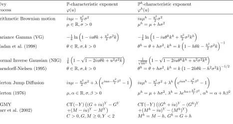
L´evy P-characteristic exponent Ph-characteristic exponent

process ϕ(u) ϕh_(u)

Arithmetic Brownian motion iuµ−u₂2σ2 _iuµh₋u2

2σ 2

µ∈R, σ >0 µh=µ+hσ2

Variance Gamma (VG) −1 kln

1−iuθk+u2

2σ

2_{k −}1 kln

1−iuθh_kh₊u2

2σ 2_kh

Madan et al. (1998) θ∈R, σ, k >0 θh=θ+hσ2,kh=k

1−hθk−h2

2σ 2_k−1

Normal Inverse Gaussian (NIG) 1_k

1−√1−2iuθk+u2_σ2_{k √}1 kkh

1−√1−2iuθh_kh_+u2_σ2_kh

Barndorff-Nielsen (1995) θ∈R, σ, k >0 θh=θ+hσ2,kh=k 1−2hθk−h2σ2k−1/2

Merton Jump Diffusion iuµ−u2

2σ 2_+λ

eiuα−u

2 2β

2

−1

iuµh₋u2

2σ 2_+λh

eiuαh−u

2 2β

2

−1

Merton (1976) µ, α∈R, σ, β >0 µh=µ+hσ2,λh=λehα+

h2

2β2,αh=α+hβ2

CGMY CΓ(−Y) (G+iu)Y _−GY _{CΓ(−Y) (G}h_+iu)Y _−(Gh₎Y

Carr et al. (2002) +(M−iu)Y −MY +(Mh−iu)Y −(Mh)Y

C >0, G, M≥0, Y <2 Mh=M−h,Gh=G+h

Table 1: Entries summarize the characteristic exponent for each L´evy process specification under both

Pand the Esscher measure of parameterh,Ph.

The Esscher change of measure is formalized in the following.

Proposition 4 Let Λ(t) and L(t) be multivariate L´evy processes as given in Proposition 1; further, let Phj be an equivalent probability measure defined by the density process

η(t) = dP hj dP Ft

=e−ϕLj(−ihj)t+hjLj(t)

, hj ∈R,

for any j= 1,· · ·, n. Then, Λ(t) andL(t)remain L´evy processes under Phj. Further, the components of Λ(t) under Phj for any j= 1,· · ·, n have characteristic exponent

ϕhj

Yj(u) = iu

βj+hjσj2+

Z

R

y(ehjy_−1)ν

j(dy)

−u 2 2 σ 2 j + Z R

eiuy−1−iuy ehjy_ν

j(dy)

ϕhj

Yk(u) = ϕYk(u), k6=j, k= 1,· · · , n ϕhj

Z(u) = iu

βZ+hjajσ2Z+

Z

R

z(ehjajz_−1)ν

Z(dz)

−u 2 2 σ 2 Z+ Z R

eiuz−1−iuz

ehjajz_ν

Z(dz).

Proof. See Appendix A.4

The corresponding characteristic exponents of the components ofL(t) underPhj follow from Propo-sition 1 and Corollary 2 (see also Eberlein et al., 2009).

Proposition 4 implies that L´evy processes are invariant under an Esscher change of measure; in other words any L´evy process remains L´evy after an appropriate redefinition of the process parameters.

A direct consequence of Proposition 4 (and the condition in equation 4) is

Ehj

eLk(t)−tϕ_Lk(−i)

=eqhjt _{k6=j (8)}

with

qhj =hjCov(Lk(1), Lj(1)) +

∞

X

n=3

n−1

X

l=1

an_k−lhl jalj

l!(n−l)!

Z

R

znνZ(dz). (9)

The result follows from the Taylor expansion of the exponential function about the origin and the

binomial theorem. This result will be useful in Section 3.3.1 in order to gauge the impact of dependence on the so called ‘quanto adjustment’.

Unless otherwise stated, all the assumptions listed in this section hold throughout the rest of the

paper.

3

A multivariate L´

evy (extended) Foreign Exchange market

3.1 The general setting

Consider a frictionless and arbitrage free market in whichN currencies are traded. In what follows, we use the convention that the spot FX rate between the l-th and them-th currency, Xm|l(t), is quoted as the amount of currency (l) per unit of currency (m). Further, we assume that interest rates are constant and we letrl>0,l= 1,· · · , N denote the continuously compounded interest rate in thel-th currency.

For the purpose of including the pricing of Quanto products, we also consider an assetS(t) traded in the market using the l-th currency. Hence, the total number of assets considered is n = N + 1. We note that for ease of exposition and notation, in the following we consider only the case of one

underlying asset; however, the model can be generalized to the case of sayM assets, so thatn=N+M. In order to model the risk dynamics of S(t) and Xm|l(t), let LS(t), LXk|l(t), k6=l

be a L´evy

process inRn with dependent components and respecting the construction given in Proposition 1, so that

Lj(t) =Yj(t) +ajZ(t), j=S, Xk|l, k6=l.

As shown in Section 2, the full description of

LS(t), LXk|l(t), k6=l

depends on the idiosyncratic risk

processes

YS(t), YXk|l(t), k6=l

and the systematic risk processZ(t); hence for simplicity of notation, we focus only on the properties of these components.

Finally, let Pl be the risk neutral martingale measure defined by the l-th currency. We note that the proposed market model is incomplete and consequently the risk neutral martingale measure is not unique. Hence, we follow standard practice for incomplete markets and fix the risk neutral

measure with respect to the chosen currency through the prices of derivative contracts traded in the

the characteristic exponents are therefore

ϕl_Yj(u) = −u

2

2 σ

2

j +

Z

R

(eiuy−1−iuy)νj(dy) j =S, Xk|l, k6=l (10)

ϕl_Z(u) = −u

2

2 σ

2

Z+

Z

R

(eiuz−1−iuz)νZ(dz). (11)

We note that in the interest of highlighting the generality of our approach, in the following we refer to the characteristic exponentϕ·(u) in its general formulation as from the L´evy-Khintchine representation

(see Section 2). For practical purposes, this exponent admits closed form expression in all the cases

of processes usually adopted in the finance literature, as the ones reported for example in Table 1. In this set-up, the index quoted in thel-th currency,S(t), and the FX spot rateXm|l_{(t) under the} risk neutral measure Pl are assumed to be of the form

S(t) = S(0)eµSt+LS(t)_{, S(0)>0}

Xm|l(t) = Xm|l(0)eµXm|lt+LXm|l(t)_{, X}m|l_(0)>0

with

µS = rl−ϕlLS(−i) =rl−ϕ

l

YS(−i)−ϕ

l

Z(−aYSi), µXm|l = rl−rm−ϕ

l L_Xm|

l(

−i) =rl−rm−ϕlY_Xm|

l(

−i)−ϕl_Z(−aXm|li).

This choice guarantees that e−rlt_{S(t) and e}−(rl−rm)t_Xm|l_{(t) (i.e. the discounted value of one unit of}

currency (m) invested in them-denominated currency money market account and converted in the (l) currency) are Pl-martingales.

Up to now, the given market is specified under the risk neutral measure defined by thel-th currency; for practical purposes it is at times convenient to change the measure to any other one based on a

num´eraire denominated in any other of theN currencies included in the FX market. Without loss of generality, we consider the risk neutral martingale measure defined by them-th currency. In the given framework, due to the change-of-num´eraire method introduced by Geman et al. (1995), Pm ∼ Pl is defined by the density process

η(t) = dP m

dPl

_F

t

= e

rmt_Xm|l_(t) erltXm|l(0)

= e

−ϕl

LX_m|l(−i)t+LXm|l(t)

. (12)

denoted by ϕm_· , follow directly from Proposition 4.

ϕm_Y

Xm|l

(u) = iu

σ2_X

m|l+ Z

R

y(ey−1)νXm|l(dy)

−u

2

2 σ

2 Xm|l+

Z

R

(eiuy−1−iuy)eyνXm|l(dy) (13)

ϕmYj(u) = −

u2 2 σ 2 j + Z R

(eiuy−1−iuy)νj(dy) j=S, Xk|l, k6=l, m (14)

ϕmZ(u) = iu

aXm|lσ 2 Z+

Z

R

z(eaXm|lz_−1)ν

Z(dz) −u 2 2 σ 2 Z+ Z R

(eiuz−1−iuz)eaXm|lz_ν

Z(dz). (15)

In the case of the processes considered in Table 1, these exponents admit closed form expressions reported in the last column of Table 1 by settingh= 1.

We note that the proposed multivariate FX model is consistent in terms of symmetries with respect

to inversion and triangulation. The result is formalized in the following.

Proposition 5 a) Symmetry with respect to inversion. Let Xl|m(t) = 1/Xm|l(t) be the “flipped” FX rate; consider the probability measure Pm defined by (12). Then underPm

Xl|m(t) =Xl|m(0)e

(rm−rl−ϕm_LX l|m

(−i))t+L_Xl|

m(t)

, (16)

for LXl|m(t) = YXl|m(t) +aXl|mZ(t), YXl|m independent of Z(t) and aXl|m = −aXm|l. Further, the component processes have characteristic exponents ϕm_Y

Xl|m

(u) = ϕm_Y Xm|l

(−u) and ϕm_Z(u) for ϕm

Y_Xm |l

(u), ϕm

Z(u) as in equations (13)-(15).

b) Symmetry with respect to triangulation. Let Xm|g(t) = Xm|l(t)/Xg|l(t) be inferred cross rate; further define Pg∼Pl by

ξ(t) = dP g

dPl

_F t =e

−ϕl

LX_g|l(−i)t+LXg|l(t) .

Then under Pg

Xm|g(t) =Xm|g(0)e

(rg−rm−ϕg_LX m|g

(−i))t+L_Xm|

g(t)

, (17)

for LXm|g(t) = YXm|g(t) +aXm|gZ(t), YXm|g independent of Z(t) and aXm|g = aXm|l −aXg|l. Further, the component processes have characteristic exponents

ϕg_Y

Xm|g

(u) = ϕY_Xm|

l(u) +ϕ

g Y_Xg

|l

(−u) (18)

ϕg_Y

Xg|l

(u) = iu

σ_X2

g|l+ Z

R

y(ey−1)νXg|l(dy)

−u

2

2 σ

2 Xg|l+

Z

R

(eiuy−1−iuy)eyνXg|l(dy) (19)

ϕg_Z(u) = iu

aXg|lσ 2 Z+

Z

R

z(eaXg|lz−_1)ν

Z(dz) −u 2 2 σ 2 Z+ Z R

(eiuz−1−iuz)eaXg|lz_ν

Z(dz). (20)

Proof. See Appendix A.5.

Same consideration as above holds for the recovery of the characteristic exponents in closed form.

These symmetries ensure that for the cases in which options on the inferred rates are actively traded in the market, the proposed model is able to consistently reprice vanilla options written on the different

3.2 Pricing FX options: implied correlation

The framework introduced in the previous section leads to analytical results (up to a Fourier inversion) for the price of vanilla options on FX rates. More precisely, consider a call option on a generic FX rate

Xm|l(t) struck atKm|l and maturityT. By risk neutral valuation, the option premium (expressed in the relevantl-th currency) is

C(Km|l, T) =e−rlT

El[(Xm|l(T)−Km|l)+]; (21)

for the computation of the above, the Carr and Madan (1999) methodology can be adopted so that

C(Km|l, T) = e

−αlnKm|l π

Z ∞

0

e−ivlnKm|lψl_m|l(v)dv, (22)

ψl_m|l(v) = e

−rlT_φl

m|l(v−(α+ 1)i;T)

α2_+α−v2_{+i(2α+ 1)v} , (23)

with

φl_m|l(u;T) =eiulnX m|l₍₀₎₊

iuµ_Xm|l+ϕl

Ym|l(u)+ϕ l Z(am|lu)

T

, (24)

and α a dampening coefficient. The relevant characteristic exponents are obtained by applying equa-tions (10)-(11).

The option pricing equations (22)-(23) show that the FX option price is necessarily a function of

both the idiosyncratic and the systematic factors composing the margin process driving the relevant

FX rate. This implies that model calibration is non-trivial as these factors are not directly observable in the market. However, in the context of the setting introduced in Section 3, due to the highlighted

symmetry with respect to triangulation, the proposed model allows a simple and effective way to

solve this problem as, in presence of actively traded options on the inferred cross rates, the required information on the risk factors can be recovered by simultaneous calibration to the three market

volatility surfaces. For the case of the cross rate Xm|g(t) given in the previous section, in fact, the option pricing formulas (22)-(23) can be restated as

C(Km|g, T) = e

−αlnKm|g π

Z ∞

0

e−ivlnKm|gψ_mg_|g(g)dv, (25) (26)

ψ_mg_|g(v) =

e−rgT_φg

m|g(v−(α+ 1)i;T)

α2_+α−v2_{+i(2α+ 1)v} , (27)

where

φg_m|g(u;T) =eiuln(X

m|g₍₀₎₎₊

iuµ_Xm|g+ϕg

Ym|g(u)+ϕ g Z(am|gu)

T

, (28)

µXm|g = rg −rm −ϕ

g L_Xm

|g

(−i), and the relevant characteristic exponents are given by equations (18)-(20).

calibrated and target implied volatilities, denoted σmod and σmkt respectively. σmod is recovered by inversion of the Black-Scholes formula in correspondence of input prices computed using the pricing

formulas above. We choose a norm in implied volatility rather than a norm in price as to avoid the introduction of bias due to the large numerical range of option price - for a detailed discussion we refer

to De Col et al. (2013) and references therein. Consequently, the objective function of our calibration

problem is

F(ˆθ) = X i

X

j

σmod

Xm|l, K_im|l, Tj; ˆθm|l

−σmkt

Xm|l, K_im|l, Tj

2

+X i

X

j

σmod

Xg|l, K_ig|l, Tj; ˆθg|l

−σmkt

Xg|l, K_ig|l, Tj

2

+X i

X

j

σmod

Xm|g, K_im|g, Tj; ˆθ

−σmkt

Xm|g, K_im|g, Tj

2

, (29)

where we sum the total number of possible strikes and maturities available for each contract in the

dataset (which we omit in the interest of readability). In equation (29) ˆθ is an element of the set of feasible vectors Θ defined as

Θ ={θˆ= (Y_m|l,Y_g|l,Z, am|l, ag|l)∈Rn¯m|l+¯ng|l+¯nZ+2 |c(ˆθ)},

where Y_m|l, Yg|l and Z are the parameter sets describing the idiosyncratic and systematic risk fac-tors of the relevant FX rates, ˆθ_m|l and ˆθg|l refer resp. to the components ˆθm|l = (Ym|l,Z, am|l) and

ˆ

θg|l = (Yg|l,Z, ag|l) of ˆθ ∈Θ, ¯n· is the number of parameters describing the process of choice for the

idiosyncratic and systematic factors (from Table 1 we observe, for example, that in the case of the VG process ¯n·= 3), andc(ˆθ) denotes the vector of all possible constraints on the parameters (like the

ones listed in Table 1 for the processes presented therein). Finally, the optimization problem used to estimate the model parameters can be stated as follows

min

ˆ

θ∈Θ

F(ˆθ). (30)

As a result of this procedure, we can also recover as a by product the implied correlation between

the relevant FX rates.

3.3 Quanto products: quanto adjustment and implied correlation

3.3.1 Quanto futures

In the following, we show how to recover market consistent information on the dependence structure between FX rates and the index S via Quanto products. As Quanto futures are the most frequently traded contracts, we analyse their pricing in the proposed setting as to gain insight into the quanto adjustment.

To this purpose, given that Quanto futures involve only one underlying asset and one FX rate, in

in Section 3.1, with only two currencies: the domestic currency (d), and the foreign (f) currency. Further, for simplicity of notation, we drop the sub-indices from all processes involved, so that under

the Foreign Risk Neutral (FRN) martingale measurePf, the underlying asset price att >0 is

S(t) =S(0)eµfSt+LS(t)_{, S(0)>0;}

in accordance with the notation introduced in Section 3.1, the relevant spot FX rate isXd|f(t) defined as

Xd|f(t) =Xd|f(0)eµfXt+LX(t), Xd|f(0)>0,

with

µf_S = rf −ϕfYS(−i)−ϕ

f

Z(−aSi),

µf_X = rf −rd−ϕfYX(−i)−ϕ

f

Z(−aXi).

It follows by standard no-arbitrage arguments that the price in the foreign economy at timet≥0 of the futures on S with maturity T equals

Ff(S;t, T) =erf(T−t)_{S(t); (31)}

similarly, under the assumption that the applied FX rate between the two currencies is set to 1d/f(see Giese, 2012, for example), the Quanto futures price in the domestic economy (i.e. under the Domestic

Risk Neutral - DRN - martingale measure Pd) is given by

Fd(S;t, T) = Ed[S(T)| Ft]

= eq(T−t)Ff(S;t, T), (32)

where q is the quanto adjustment given by

q=Covf(LS(1), LX(1)) +

∞

X

n=3

n−1

X

l=1

an_S−lal_X l!(n−l)!

Z

R

znνZ(dz), (33)

in virtue of equations (8)-(9) with hj = 1. In this respect, we note that, in the case in which the driving processes are all Brownian motions (i.e. continuous processes with no jumps), the quanto adjustment reduces to the well known “Black-Scholes type” quanto adjustment

q=aSaXσZ2 =ρSX

p

Var(LX(1))Var(LS(1)), (34)

and therefore it only depends on the linear pairwise correlation coefficient between the relevant driving processes. In the more general case, though, equation (33) shows that the quanto adjustment also

depends on higher order cumulants of the pure jump part of the systematic risk process calculated

on the “implied” correlation existing between the log-returns of the index and spot FX rate.

The previous observation leads to a 2-step calibration procedure structured as follows. In first

place, we assume that in the market there are Quanto futures prices onM different underlying assets (S1, ..., SM); further, we assume that the M assets are traded in the foreign market with currencyf. The Quanto futures are instead cash settled and traded in the domestic currency d. Thus, the first step consists in the calibration of the parameters of the systematic risk process, Z, and the loading factors (a1, . . . , aM, aX) using Quanto futures. With a similar notation to the one adopted in Section 3.2, this is achieved by defining the objective function F(ˆθ) as

F(ˆθ) =X i

X

j

F_modd (Si, t, Tj; ˆθ)−F_mktd (Si, t, Tj)

Fd

mkt(Si, t, Tj)

!2

, (35)

and solving the optimization problem

min

ˆ

θ∈Θ

F(ˆθ) (36)

with

Θ ={θˆ= (Z, a1, . . . , aM, aX)∈R¯nZ+M+1|c(ˆθ)}.

Conditioned on the parameters values obtained in the first step, the second step is given byM+ 1 independent minimization problems, one per each asset S and the FX rate, aimed at recovering the parameters of the idiosyncratic components. In more details, we achieve this by calibration to the implied volatility surfaces of the corresponding margin processes; consequently, the relevant objective

functions are

Fi(ˆθYi) =

X

k

X

l

σmod

Si, Ki,k, Ti,l; ˆθYi

−σmkt(Si, Ki,k, Ti,l)

2

i= 1, . . . , M (37)

FX(ˆθYX) =

X

k

X

l

σmod

Xd|f, Kk, Tl; ˆθYX

−σmkt

Xd|f, Kk, Tl

2

. (38)

Note the different norm in equation (35); this is to ensure consistency in scale with equations (37)-(38)

as to avoid the introduction of bias also in this case (see previous section). The actual calibration is

the solution to the optimization problems

min

ˆ

θ_Yi∈Θ_Yi

Fi(ˆθYi), i= 1, . . . , M (39)

min

ˆ

θ_YX∈Θ_YX

FX(ˆθYX) (40)

with

ΘYi = {θˆYi =Yi∈R

¯

ni _|c(ˆθ

Yi)}, i= 1, . . . , M

ΘYX = {θˆYX =YX ∈R

¯

nX _|c(ˆθ

YX)}.

dimension of the vector ˆθ, the first step of the calibration procedure described above is ill-posed. In this situation, we recommend a joint calibration formulated as follows

min

ˆ

θ∈Θ,θˆ_Yi∈Θ_Yi,i=1,...,M,θˆ_YX∈Θ_YX

F(ˆθ) +X i

Fi(ˆθYi) +FX(ˆθYX). (41)

Alternatively to the calibration procedure described above which is essentially based on the idea of recovering information on the dependence in place using Quanto futures, one could instead resort to

common market practice of using historical correlation/covariance between the variables of interest.

In this case, the objective function will have to be restated in terms of fitting the non diagonal entries of the sample covariance matrix to their theoretical counterpart predicted by the multivariate model.

This is achieved by redefining the objective function of the first step described above, i.e. equation

(35), as follows

FC(ˆθ) =kCovmod(S, X; ˆθ)−Covmkt(S, X)kF (42) and solving the optimization problem

min

ˆ

θ∈Θ

FC(ˆθ), (43)

where k · kF denotes the Frobenius norm, Covmod(·) = aa0Var(Z(1)) is the model covariance matrix between the index log-returns and the FX log-rate,Covmkt(·) is the corresponding observed covariance matrix. Similarly to the case described above, if the number of quotes is less than the dimension of

ˆ

θ, we recommend a joint calibration similar to what stated in equation (41) in which F(ˆθ) is replaced by FC(ˆθ).

In order to distinguish between the two procedures in the following sections, the calibration based

on the optimization problems (36), (39), (40) (alternatively 41) is referred to as`QF-based calibration´; instead, we refer to the calibration which uses the optimization problem (43) as first step as`HC-based calibration´.

3.3.2 Pricing Quanto options

In this section we provide a possible way of back-testing the QF-based and HC-based calibration procedures introduced in the previous section. The idea is to verify the consistency of the information

retrieved from the two procedures using the prices of other Quanto products such as Quanto options.

The arbitrage free price of a (European type) Quanto call option on the (Quanto) futures on the assetS, expressed in units of domestic currency, is given by

QC(Fd(S;T1, T2), K, T1) =e−rdT1Ed[(Fd(S;T1, T2)−K)+]

where Fd_(S;T

1, T2) is the Quanto futures price at timeT1 with maturity T2;T1 ≤T2 is the maturity

of the option contract.

It follows from equation (32) that

with

Qadj = e(rf+q)(T2−T1),

K∗ = K

Qadj

.

A Quanto call option can therefore be seen as a vanilla call onS struck atK∗, rescaled by a constant,

Qadj, incorporating the quanto adjustment. As in the market model under consideration relevant characteristic functions are available (see for example Table 1), the price in equation (44) can be computed efficiently by means of Fourier inversion based methods, such as the Carr-Madan approach

(Carr and Madan, 1999) for example. In this respect, we note that the large majority of options

offered on the CME are of American type; the early exercise property can be accommodated in the pricing by adopting either the CONV method of Lord et al. (2008) or the COS method of Fang and

Oosterlee (2009) for example; alternatively the so called extension method of Fabozzi et al. (2016) could be used as well. This is left though to future research.

4

Numerical results

4.1 Setup

In this section, we analyze the performance of our model in terms of calibration, pricing and impact

on risk management, using real market quotes. We consider two currency triangles - EUR/USD/CHF

as on 17/03/2016 and MXN/USD/ZAR as on 21/12/2016, and two Quanto futures products - the USD-denominated Quanto futures on the Nikkei 225 index observed on 13/06/2014, and the

ZAR-denominated Brent Crude Oil Quanto futures observed on 15/04/2016. The South African Rand (ZAR) and the Mexican Peso (MXN) can be classified as emerging markets currencies1_{. The}

USD-denominated Quanto futures on the Nikkei 225 index are traded on the CME with quarterly maturities

(i.e. March, June, September and December) on the second Friday of the contract month; the minimum price change (tick) is 5 index points. Finally, they are characterized by a multiplier of 5 USD for

Dollar-denominated CME Nikkei 225 Futures; for more details see e.g. Co et al. (2013). The Brent Crude Oil

Quanto futures is traded on the JSE and is a Brent crude oil futures contract that is cash settled and traded in ZAR, but mimics the performance of the foreign referenced USD price of Brent crude oil as

traded on NYMEX, a subsidiary of the CME Group Inc. Contract months are February, May, August

and November; expiry date is the 15th business day prior to the first business day of the next calendar month. Relevant data are summarized in Table 2. Note that in the interest of space we report the

market quotes of the relevant products in Appendix B.

This analysis uses the model calibration procedure introduced in the previous sections; for illus-tration purposes, we choose as relevant L´evy process the VG process of Madan et al. (1998). In some

more details, the VG process is a normal tempered stable process obtained by subordinating a

Brown-ian motion with drift by an independent (unbiased) Gamma process. From Table 1 the characteristic

March 17, 2016 USDCHF-EURCHF

USDCHF Xm|l(0) 0.96 CHF/USD EURCHF Xg|l_{(0) 1.09 CHF/EUR} USDEUR Xm|g(0) 0.88 EUR/USD US risk free rate of interest rm 0.5%

EUR risk free rate of interest rg 0% SWISS risk free rate of interest rl 0% Historical correlation ρh_Xm|l_Xg|l 45%

December 21, 2016 USDZAR-MXNZAR

USDZAR Xm|l(0) 14.0824 ZAR/USD MXNZAR Xg|l_{(0) 0.6892 ZAR/MXN} USDMXN Xm|g(0) 20.4330 MXN/USD US risk free rate of interest rm 0.75%

South African risk free rate of interest rd 7% Mexican risk free rate of interest rl 5.75 %

Historical correlation ρh_Xm|l_Xg|l 56.72%

June 13, 2014 Nikkei 225-USDJPY

Nikkei 225 S(0) 15097.84 JPY USDJPY X(0) 102.03 JPY/USD Japan risk free rate of interest rf 0.10%

US risk free rate of interest rd 0.25%

Nikkei 225 futures (Sept) Ff(S; 0, T) 15030 JPY Nikkei 225 Quanto futures (Sept) Fd_{(S; 0, T) 15065 USD}

T 12/09/2014 Historical correlation ρhSX 28%

April 15, 2016 BRENT-ZARUSD

BRENT S(0) 43.72 USD ZARUSD X(0) 0.0687 USD/ZAR US risk free rate of interest rf 0.5%

South African risk free rate of interest rd 7%

BRENT futures (May) F1f(S; 0, T1) 43.73 USD BRENT futures (Aug) F₂f(S; 0, T2) 43.79 USD BRENT Quanto futures (May) Fd

1(S; 0, T1) 43.78 ZAR BRENT Quanto futures (Aug) Fd

2(S; 0, T2) 44.37 ZAR

T1 10/05/2016

T2 11/08/2016 Historical correlation ρhSX 31.4%

Table 2: Synopsis of market data. Source: Bloomberg, CME free web platform (see http://www.cmegroup.com/). r.: benchmark interest rates. ρh: historical correlation between log-returns estimated on a sample size of 128 days. Note: as the benchmark Swiss interest rate is negative at the observation date, we assume this rate to be zero.

exponent reads

ϕ(u) = −1

kln

1−iukθ+u2σ

2

2 k

, u∈_R, (45)

and excess kurtosis are

skew(t) = θ 3σ

2_{k+ 2θ}2_k2

(σ2_+θ2_k)3/2√_t, kurt(t) =

3k σ4+ 4σ2θ2k+ 2θ4k2

(σ2_+θ2_k)2_t .

From the above we observe that the parameter θ ∈ R determines the sign of the skewness of the distribution of the VG process,σ >0 controls the overall variance level andk >0 governs the kurtosis or tail heaviness of the distribution.

For the implementation of the market model introduced in Section 3, we assume that both the

sys-tematic risk process and all the idiosyncratic risk processes of interest follow a VG process respectively

with parameters (θZ, σZ, kZ) and (θYj, σYj, kYj) for j =S, Xk|l, k 6= l, under the relevant probability

measure. In particular, we notice that under these assumptions, equations (32)-(33) imply

Fd(S;t, T) =Ff(S;t, T)eq(T−t), (46)

with

q = 1

kZ

ln 1−aXkZθZ−

1

2kZa2Xσ2Z

1−aSkZθZ−1₂kZa2_Sσ_Z2

1−(aS+aX)kZθZ−1₂kZ(aS+aX)2σZ2

!

. (47)

The results of the several calibration procedures carried out in this numerical experiment are reported in Tables 3-6. At this stage we pay particular attention to the calibration errors: in order to

carry out a meaningful comparison given the different nature of the assets involved (FX rates, market

indices and futures), we express the Root Mean Square Error (RMSE) reported in Tables 3-6 as percentage of the ATM (Delta neutral) implied volatility (reported in Appendix B). The calibrations

based on market information and the ones based instead on historical information generate relatively

similar error for all cases considered in this experiment: the errors, in fact, range from 0.12% (in the case of the USDZAR FX rate) to 1.66% (for the case of the USDJPY FX rate). Although these errors

are relatively small, even in the case of emerging markets currencies such as ZAR and MXN generally

characterized by significantly higher volatilities, the different source of information used (market vs historical) has a more subtle impact which is analysed in fuller details in the following sections.

4.2 FX Triangles

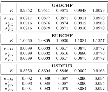
We implement the calibration procedure introduced in Section 3.2 for the specific case of the currency triangles EUR/USD/CHF and MXN/USD/ZAR. For this purpose we consider vanilla options on

these FX rates with maturity 1 month. Following FX conventions, all quotes, which are taken from

Bloomberg, are expressed in terms of Delta; specifically we use the Delta Neutral and the 10 and 25 Delta Call and Put market quotes, which are converted in strikes following the procedure described

in Bossens et al. (2010).

Tables 3-4 report the model parameters obtained by the joint calibration to FX triangle, i.e. the solution to the optimization problem stated in equations (29)-(30). We denote this calibration

TRIANGLE-based calibration HC-based calibration

Idiosyncratic process Systematic process Idiosyncratic process Systematic process

USDCHF EURCHF USDCHF EURCHF

θY 0.1180 0.0632 θZ -0.2846 θY 0.0172 0.0096 θZ 0.0863

σY 0.0724 0.0451 σZ 0.3859 σY 0.0665 0.0519 σZ 0.2920

κY 0.0326 0.1244 κZ 0.1504 κY 0.0690 0.2990 κZ 0.0610

a 0.1289 0.1169 a 0.2132 0.1551

RMSE 0.34% 0.49% (0.0003) RMSE 0.46% 0.65% (0.0004)

ρi,V G

Xm|lXg|l 0.3857 ρ

h,V G

Xm|lXg|l 0.4486

Margin process Systematic process Margin process Systematic process

USDCHF EURCHF USDCHF EURCHF

EL(1) 0.0813 0.0300 EZ(1) -0.2846 EL(1) 0.0357 0.0230 EZ(1) 0.0863

p

VarL(1) 0.0915 0.0688 pVarZ(1) 0.4013 pVarL(1) 0.0913 0.0692 pVarZ(1) 0.2927

s(L(1)) 0.0270 0.0726 s(Z(1)) -0.3120 s(L(1)) 0.0380 0.0861 s(Z(1)) 0.0539

κ(L(1)) 0.1051 0.2564 κ(Z(1)) 0.5170 κ(L(1)) 0.0997 0.3309 κ(Z(1)) 0.1850

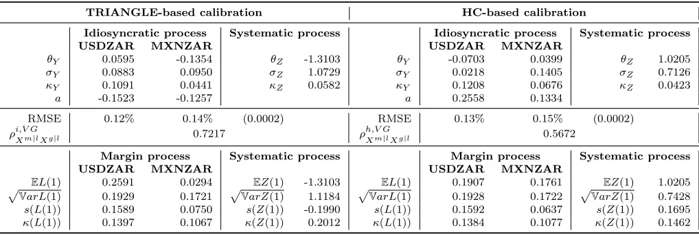
Table 3: Top panel - Calibrated parameters of the multivariate VG model. TRIANGLE-based calibra-tion: solution to optimization problem (29) - (30). HC-based calibracalibra-tion: Z,aS, aX calibrated using historical correlation (128 days). Bottom panel - Moments of the resulting margin distribution. RMSE: percentage of the ATM Delta neutral implied volatility (RMSE actual value in parenthesis) - USDEUR: 0.34% (TRIANGLE-based calibration), 0.46% (HC-based calibration). ρi,V G_Xm|l_Xg|l: pairwise correlation coefficient from equation (5) and the TRIANGLE-based calibrated parameters. ρh,V G_Xm|lXg|l: recovered pairwise historical correlation. s, κ: indices of skewness and excess kurtosis as in Cont and Tankov (2004). Data: see Tables 2 and B.1.

TRIANGLE-based calibration HC-based calibration

Idiosyncratic process Systematic process Idiosyncratic process Systematic process

USDZAR MXNZAR USDZAR MXNZAR

θY 0.0595 -0.1354 θZ -1.3103 θY -0.0703 0.0399 θZ 1.0205

σY 0.0883 0.0950 σZ 1.0729 σY 0.0218 0.1405 σZ 0.7126

κY 0.1091 0.0441 κZ 0.0582 κY 0.1208 0.0676 κZ 0.0423

a -0.1523 -0.1257 a 0.2558 0.1334

RMSE 0.12% 0.14% (0.0002) RMSE 0.13% 0.15% (0.0002)

ρi,V G

Xm|l_Xg|l 0.7217 ρ

h,V G

Xm|l_Xg|l 0.5672

Margin process Systematic process Margin process Systematic process

USDZAR MXNZAR USDZAR MXNZAR

EL(1) 0.2591 0.0294 EZ(1) -1.3103 EL(1) 0.1907 0.1761 EZ(1) 1.0205

p

VarL(1) 0.1929 0.1721

p

VarZ(1) 1.1184

p

VarL(1) 0.1928 0.1722

p

VarZ(1) 0.7428

s(L(1)) 0.1589 0.0750 s(Z(1)) -0.1990 s(L(1)) 0.1592 0.0637 s(Z(1)) 0.1695

κ(L(1)) 0.1397 0.1067 κ(Z(1)) 0.2012 κ(L(1)) 0.1384 0.1077 κ(Z(1)) 0.1462

Table 4: Top panel - Calibrated parameters of the multivariate VG model. TRIANGLE-based calibra-tion: solution to optimization problem (29) - (30). HC-based calibracalibra-tion: Z,aS, aX calibrated using historical correlation (128 days). Bottom panel - Moments of the resulting margin distribution. RMSE: percentage of the ATM Delta neutral implied volatility (RMSE actual value in parenthesis) - USDMXN: 0.17% (TRIANGLE-based calibration), 0.19% (HC-based calibration). ρi,V G_Xm|l_Xg|l: pairwise correlation

coefficient from equation (5) and the TRIANGLE-based calibrated parameters. ρh,V G_Xm|l_Xg|l: recovered pairwise historical correlation. s, κ: indices of skewness and excess kurtosis as in Cont and Tankov (2004). Data: see Tables 2 and B.2.

generated by the calibrated model are within the corresponding market bid and ask volatilities for

both the main currency pairs and the inferred cross rate.

As to highlight the importance of using market consistent information on dependence (in this case as extracted from the currency triangle), we compare these results with the ones obtained under

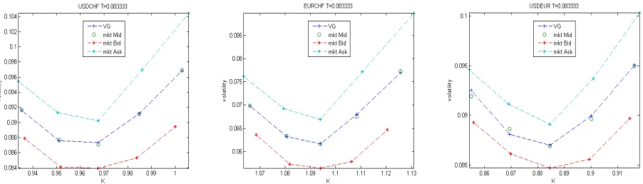
Figure 1: USDCHF, EURCHF and USDEUR implied volatility in function of strike K: market vs calibrated multivariate VG model. Options market data, March 17, 2016: Source: Bloomberg. Options maturity: T = 1month. Market Data: Tables 2 and B.1. Multivariate VG model parameters: Table 3, TRIANGLE-based calibration.

Figure 2: USDCHF, EURCHF and USDEUR implied volatility in function of strike K: market vs calibrated multivariate VG model. Options market data, March 17, 2016: Source: Bloomberg. Options maturity: T = 1month. Market Data: Tables 2 and B.1. Multivariate VG model parameters: Table 3, HC-based calibration.

correlation in a way similar to the HC-based calibration procedure illustrated in Section 3.3.1. This

would be necessary for example in absence of liquidly traded options on the inferred cross rate. The historical correlation between the FX log-rates is estimated using the sample correlation, denoted as

ρh_Xm|l_Xg|l, based on a sample size of 128 days - which is reported in Table 2 (although in Section

3.3.1 the measure of linear dependence used is the historical covariance, for ease of exposition in the remaining of the paper we convert this measurement into historical correlation).

Although the two calibration procedures generate very similar errors, as noted above, there is

a noticeable discrepancy between the value of the implied correlation resulting from the calibration based on the triangles (38.6% and 72.2% respectively) and the historical estimate obtained using the

sample correlation (45% and 56.7% respectively). Further, when the parameters from the HC-based

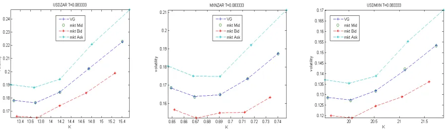
calibration are used to reproduce the smile of the inferred cross rate, the resulting curve violates the bounds given by the market bid and ask volatilities as illustrated in Figure 2 and 4 - last panel on the

Figure 3: USDZAR, MXNZAR and USDMXN implied volatility in function of strikeK: market vs calibrated multivariate VG model. Options market data, December 21, 2016: Source: Bloomberg. Options maturity: T = 1month. Market Data: Tables 2 and B.2. Multivariate VG model parameters: Table 4, TRIANGLE-based calibration.

Figure 4: USDZAR, MXNZAR and USDMXN implied volatility in function of strikeK: market vs calibrated multivariate VG model. Options market data, December 21, 2016: Source: Bloomberg. Options maturity: T = 1month. Market Data: Tables 2 and B.2. Multivariate VG model parameters: Table 4, HC-based calibration.

4.3 Quanto futures

4.3.1 Nikkei 225

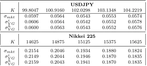
We use market data from Bloomberg and the CME free web platform observed on June 13, 2014. Vanilla options on the Nikkei 225 index have maturity of 28 days (July 11, 2014) as these quotes were

the most liquid in the market2; consequently, we have chosen vanilla options on the USDJPY FX rate

with similar maturity, regardless of the fact that the FX market shows high liquidity across other maturities as well. In particular, we consider 9 different strikes for the Nikkei 225 index options and

5 different strikes for the USDJPY exchange rate options. The futures contracts considered have a

maturity in 91 days (September 12, 2014); similarly to the previous section, the historical correlation between the log-returns of the Nikkei 225 index and the USDJPY FX rate is estimated using the

sample correlation, denoted as ρh_SX, based on a sample size of 128 days. We just notice that the quotes of the Nikkei 225 index rates are end-of-day quotes, whereas the other quotes were observed at

3pm GMT.

Results are summarized in Table 5, in which we report the model parameters obtained from the two

alternative calibration procedures, i.e. the QF-based calibration given by the optimization problem in equations (36), (39), (40) and the HC-based calibration given by the optimization problem in equation

(43) (and 39-40). Figure 5 shows the market volatility smile and the calibrated one originated by our

multivariate VG model for both Nikkei 225 and USDJPY vanilla options with parameters from the QF-based calibration (similar results are obtained under the HC-based calibration and are available

upon request). In particular, the implied volatilities generated by the calibrated multivariate VG

model are always bounded by the corresponding market bid and ask volatilities under both calibration assumptions.

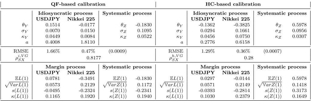
In more details, from Table 5 we observe that, although both procedures are highly accurate, the calibrated parameters generate distributions of the margin processes for the log-returns of the

Nikkei 225 index and the USDJPY FX rate which are relatively different under the two calibration

assumptions. The assets log-return distributions, in fact, are characterized by very similar volatility (meant as the square root of the process’ variance), however the Nikkei 225 index one shows a more

pronounced left skew with thicker tails under the HC-based calibration, whilst the USDJPY FX rate

distribution presents these features under the QF-based calibration. We also note that the skewness of the distribution of systematic risk process Z(t) changes sign from one calibration procedure to the other.

Finally, Table 5 reports the pairwise linear correlation coefficient between the log-returns of the Nikkei 225 index and the USDJPY spot FX rate computed on the basis of these calibrated parameters

and equation (5). We note the significant difference between the correlation coefficient implied by the

QF-based calibration, ρi,V G_SX , which returns a value of 81.77%, and the correlation generated by the HC-based calibration, ρh,V G_SX , which matches exactly the given 128-day historical correlation value at 28%. For comparison purposes, the historical correlation computed using a sample of 1 year daily data

is 37.7%, and 39.72% if a sample of 2 years daily data is considered instead. Similar discrepancies are observed when both calibration procedures are repeated overtime (see Appendix C). With hindsight,

a possible motivation for the observed differences could be traced back to the unprecedented monetary

easing policies implemented by the Japanese government aimed at ending deflation. From this simple analysis it transpires that the market was already anticipating in June 2014 the impact of these

monetary policies. Admittedly, 8 months later, in February 2015, the Nikkei Stock Average rose to a

15 years high, whilst the Yen settled around the weakest level against the US Dollar since 2007.

4.3.2 Brent Crude Oil

We use market data from Bloomberg observed on April 15, 2016. In particular, we use liquid market

quotes of vanilla options on the Brent futures (expiring on August 11, 2016) with maturity of 73

days (June 27, 2016). Furthermore, we observe vanilla options on the ZARUSD FX rate with similar maturity. We consider 20 different strikes for the options on the Brent Futures and 5 different strikes

for the ZARUSD exchange rate options. For the QF-based calibration - given by the optimization

QF-based calibration HC-based calibration

Idiosyncratic process Systematic process Idiosyncratic process Systematic process

USDJPY Nikkei 225 USDJPY Nikkei 225

θY 0.1514 -0.0177 θZ -0.1830 θY -0.1362 -0.3825 θZ 0.5978

σY 0.0070 0.0150 σZ 0.1095 σY 0.0294 0.1661 σZ 0.0956

κY 0.0449 0.0084 κZ 0.0522 κY 0.0456 0.0750 κZ 0.0307

a 0.4008 1.8110 a 0.2776 0.6158

RMSE 1.66% 0.47% (0.0009) RMSE 1.29% 0.36% (0.0007)

ρi,V G_SX 0.8177 ρh,V G_SX 0.28

Margin process Systematic process Margin process Systematic process

USDJPY Nikkei 225 USDJPY Nikkei 225

EL(1) 0.0781 -0.3491 EZ(1) -0.1830 EL(1) 0.0297 -0.0144 EZ(1) 0.5978

p

VarL(1) 0.0573 0.2129 pVarZ(1) 0.1172 pVarL(1) 0.0571 0.2149 pVarZ(1) 0.1418

s(L(1)) -0.0495 -0.2324 s(Z(1)) -0.2341 s(L(1)) -0.0393 -0.2814 s(Z(1)) 0.3173

κ(L(1)) 0.1165 0.1920 κ(Z(1)) 0.1940 κ(L(1)) 0.1030 0.2379 κ(Z(1)) 0.1649

Table 5: Top panel - Calibrated parameters of the multivariate VG model. QF-based calibration:

Z, aS, aX calibrated using Quanto futures quotes. HC-based calibration: Z, aS, aX calibrated using historical correlation (128 days). Bottom panel - Moments of the resulting margin distribution. RMSE: percentage of the ATM (Delta neutral) implied volatility (RMSE actual value in parenthesis). ρi,V G_SX : pairwise correlation coefficient from equation (5) and the QF-based calibrated parameters. ρh,V G_SX : recovered pairwise historical correlation. s,κ: indices of skewness and excess kurtosis as in Cont and Tankov (2004). Data: see Tables 2 and B.3.

May 10 and August 11, 2016. For the HC-based calibration - optimization problem in equation (43)

(and 39-40) - we estimate the historical correlation between the log-returns of the Brent and the

ZARUSD FX rate using the sample correlation based on a sample size of 128 days.

Results from both calibration procedures are summarized in Table 6; the goodness of fit is shown

in Figure 6: also in this example the recovered implied volatility smile is within the market bid-ask

spread regardless of the calibration procedure used. Similarly to the previous cases, the QF-based and HC-based calibrations originate different values of the correlation indices, which are reported in Table

6, although in this instance the discrepancy is relatively minimal, 34.6% to 31.4%. We also observe

that the relevant distribution features are quite similar under both calibration assumptions.

4.4 Implied correlation from Quanto Options

In this section, we aim at further testing the consistency of the two calibration procedures on Quanto

futures introduced in Section 3.3.1 and performed in Section 4.3 through the pricing of Quanto options. As discussed in Section 3.3.2, due to the fact that in our framework these products can be easily

priced via analytical formulas (up to a Fourier inversion), these prices can be used to back out the

relevant correlation. However, although market quotes for Quanto options are available from the CME platform, we do not have access to them and therefore we base our analysis on model prices obtained

using the parameters recovered from both calibration procedures. Then, we can recover the value of

the correlation coefficient such that the computed Quanto call option prices are matched by the ones obtained in the Black-Scholes model. To this purpose, though, we need first to carefully deal with

the volatility smile/skew effect. Common market practice is, in fact, to use the at-the-money implied

Figure 5: USDJPY and Nikkei 225 implied volatility in function of strike K: market vs calibrated multivariate VG model. Options market data, June 13, 2014: Source: Bloomberg. USDJPY Options maturity: T = 1month. Nikkei 225 Options maturity: T = 28days (July 11, 2014). Market Data: Tables 2 and B.3. Multivariate VG model parameters: Table 5, QF-based calibration.

Figure 6: ZARUSD and BRENT implied volatility in function of strike K: market vs calibrated multivariate VG model. Options market data, April 15, 2016: Source: Bloomberg. ZARUSD Options maturity: T = 2month. BRENT Options maturity: T = 73 days. Market Data: Tables 2 and B.4. Multivariate VG model parameters: Table 6, QF-based calibration.

equation (44) with Qadj = 1 in the Black-Scholes setting to recover the correlation coefficient value such that the Quanto call prices generated by the multivariate VG model are matched exactly.

We focus in particular on the case of the Nikkei 225 index, due to the large discrepancies observed

in Section 4.3.1. Results are presented in Figure 7, in which we show the implied correlation coefficient

extracted from the Black-Scholes model under the assumption that the volatility of both the Nikkei 225 index and the USDJPY FX rate is set at the corresponding at-the-money value, and under the

assumption that the volatility smile of the index is incorporated in the procedure. In details, in

the left hand side panel of Figure 7, we illustrate the case in which the input Quanto option prices are generated using the parameters from the QF-based calibration; we denote the resulting implied

correlation coefficients as ρi,BS_SX (K;v1) if at-the-money volatilities are used, and ρi,BSSX (K;v2) if the

whole volatility smile is incorporated instead. Similarly, in the right hand side panel of Figure 7 we report the same quantities obtained from input prices generated by the parameters from the

HC-based calibration; we denote these coefficients as ρh,BS_SX (K;v1) and ρh,BS_SX (K;v2). We note that when

QF-based calibration HC-based calibration

Idiosyncratic process Systematic process Idiosyncratic process Systematic process

ZARUSD BRENT ZARUSD BRENT

θY -0.2879 -0.3608 θZ -0.2089 θY -0.3136 -0.4426 θZ -0.3741

σY 0.1436 0.1300 σZ 0.3446 σY 0.1433 0.1289 σZ 0.3553

κY 0.1208 0.9995 κZ 0.1525 κY 0.1121 0.7052 κZ 0.1420

a -0.2976 -0.9733 a -0.2636 -0.8478

RMSE 1.25% 0.57% (0.0024) RMSE 1.12% 0.51% (0.0021)

ρi,V G_SX 0.3449 ρh,V G_SX 0.3137

Margin process Systematic process Margin process Systematic process

ZARUSD BRENT ZARUSD BRENT

EL(1) -0.2257 -0.1575 EZ(1) -0.2089 EL(1) -0.2150 -0.1254 EZ(1) -0.3741

p

VarL(1) 0.2043 0.5156 pVarZ(1) 0.3541 pVarL(1) 0.2042 0.5097 pVarZ(1) 0.3822

s(L(1)) -0.2976 -0.7390 s(Z(1)) -0.2651 s(L(1)) -0.2975 -0.6666 s(Z(1)) -0.3980

κ(L(1)) 0.3378 1.9232 κ(Z(1)) 0.5049 κ(L(1)) 0.3352 1.5804 κ(Z(1)) 0.5340

Table 6: Top panel - Calibrated parameters of the multivariate VG model. QF-based calibration:

Z, aS, aX calibrated using Quanto futures quotes. HC-based calibration: Z, aS, aX calibrated using historical correlation (128 days). Bottom panel - Moments of the resulting margin distribution. RMSE: percentage of the ATM (Delta neutral) implied volatility (RMSE actual value in parenthesis). ρi,V G_SX : pairwise correlation coefficient from equation (5) and the QF-based calibrated parameters. ρh,V G_SX : recovered pairwise historical correlation. s,κ: indices of skewness and excess kurtosis as in Cont and Tankov (2004). Data: see Tables 2 and B.4.

If instead the volatility smile is used, the resulting implied correlation values show an increasing pattern

from 70.91% to 79.54% in the case of input parameters obtained from the QF-based calibration, and 34.74% to 52.76% in the case of input parameters from the HC-based calibration. This shows a mild correlation skew pattern.

Figure 7: Left hand panel: QF-based calibration. Right hand panel: HC-based calibration.

ρ·_SX,BS(K;v1): Quanto call implied correlation in function of strikeK, extracted in a BS setting where the Nikkei 225 index and the USDJPY FX rate volatility are set at their at-the-money values (see Table B.3). ρ·_SX,BS(K;v2): Quanto call implied correlation in function of strikeK, extracted in a BS setting where the strike corresponding Nikkei 225 index implied volatility (Figure 5) is used. Market data: see Tables 2 and B.3.

However, from this simple experiment, we observe that once the volatility smile of the underlying asset is correctly taken into account, information extracted from historical prices generates inconsistent

estimates of the correlation value; by using the parameters obtained from the HC-based calibration, in