Geometrically Designed Variable Knot Splines in Generalized (Non-)Linear Models

City, University of London Institutional Repository

Citation

:

Geometrically Designed Variable Knot Splines in Generalized (Non-)Linear Models. .

This is the supplemental version of the paper.

This version of the publication may differ from the final published

version.

Permanent repository link: http://openaccess.city.ac.uk/18460/

Link to published version

:

Copyright and reuse:

City Research Online aims to make research

outputs of City, University of London available to a wider audience.

Copyright and Moral Rights remain with the author(s) and/or copyright

holders. URLs from City Research Online may be freely distributed and

linked to.

City Research Online: http://openaccess.city.ac.uk/ [email protected]

Online supplement to: Geometrically Designed Variable Knot

Splines in Generalized (Non-)Linear Models

Dimitrina S. Dimitrova∗a, Vladimir K. Kaisheva, Andrea Lattuadab and Richard J. Verralla

a_{Faculty of Actuarial Science and Insurance, Cass Business School, City, University of} London

b_{Department of Mathematical Sciences, Mathematical Finance and Econometrics,} Catholic University of Milan

October 30, 2017

In Section 4.1 of the paper, we tested the sensitivity of GeDS with respect to the sample size

N. In this supplement, we present the results of some further sensitivity tests and comparisons

of GeDS with existing spline methods. In Section 1, we use the data simulated as in Example 1

of the paper (see Section 4.1 therein) in order to test the sensitivity of GeDS with respect to the

choice of stopping rule and with respect to the tuning parameters β ∈(0,1) and φexit ∈ (0,1)

(see Section 3.1 of the paper and Kaishev et al. (2016)). In Section 2, we expand the numerical

comparisons of Section 4.1 of the paper including four additional test functions commonly used

in the literature (c.f. Table 3). For convenience, in what follows the stopping rules defined by

Equations (10), (9) and (11) in Section 3.1 of the paper are referred to correspondingly asratio

of deviances (RD),(exponentially) smoothed ratio (of deviances)(SR) andlikelihood ratio (test)

(LR).

1

Sensitivity tests

In this section, we test the sensitivity of GeDS with respect to the tuning parametersβ ∈(0,1) and φexit∈(0,1) and the choice of stopping rule among RD, SR and LR.

Recall that the parameterφexitis related to the model selection rule which determines when

to exit from stage A, i.e. it determines the number of knots,κ, in the knot setδκ,2 of the linear

∗

spline fit ˆf(δκ,2,αˆ;x) and hence, the number of knots of the final higher order ML spline fit

ˆ f

¯_{tκ−(n−2),n,θ}ˆ_{;x. The parameter β determines the weight put on the cluster range and the}

mean cluster size within each cluster of residuals of same sign, according to Step 6 of stage A,

and as explicitly defined in Step 5 of Kaishev et al. (2016). It therefore affects to some extent

the ordering of the cluster weights and hence, the knot placement.

In the Normal case, Kaishev et al. (2016) recommend to choose β depending on how wiggly

the underlying function f is and on the Signal to Noise Ratio (SNR), SNR= (var(f))0.5/σ.

However this approach is not appropriate in the broader framework of GLMs as it is not possible

to separately distinguish a noise component and a signal component. Moreover mean and

variance in general are not independent and observations are often significantly heteroscedastic

and there is no invariance with respect to a linear transformation of the functionf. Therefore,

as also confirmed by our sensitivity tests, the choice of β and φexit in the GLM framework

depends more complexly and jointly on the particular distribution (from the EF) of the data

and the smoothness/wiggliness of the underlying functionf. Hence, universal rules for selecting

the tuning parameters β, and φexit are difficult to formulate, although some general guidance

for the range of these parameters could still be given, as illustrated next.

For the purpose of this test we use functionf1, defined by Equation (17) in the paper, as the

“true” predictor and generate 200 samples of 500 Poisson observations as described in Example 1

of Section 4.1. Then we fitted GeDS employing the three alternative stopping rules, RD, SR

and LR in stage A of the method with different choices of the tuning parametersβ ∈(0,1) and φexit ∈ (0,1). The results of this sensitivity study are summarized in Tables 1 and 2. More

specifically, results for the RD rule with two sets of parameters, {φexit = 0.995;q = 2} and

{φexit = 0.9952;q = 4} are coded in Tables 1 and 2 as RD1 and RD2; results for the SR rule

with {φexit = 0.995;q = 2} and {φexit = 0.99;q = 2} are coded as SR1 and SR2; and the LR

rule with {φexit = 0.995;q = 2} and {φexit = 0.5;q = 2}, coded as LR1 and LR2. Note that

RD, SR and LR involve an additional parameter, q, with a default value q = 2 (c.f. Kaishev

et al. (2016)). We have tested its influence on the stopping rule and the final GeDS fits in the

GNM (GLM) framework, see Tables 1 and 2, and have concluded that it is rather modest.

Table 1 summarizes means and standard deviations (in parentheses) of the number of knots

estimated by GeDS for different stopping rules and values of the tuning parameters, φexit and

fit.

RD1 RD2 SR1 SR2 LR1 LR2

β= 0.1 12.61 17.09 16.68 13.65 9.3 15.31

(4.1) (5.94) (4.17) (3.13) (2.35) (5.25)

β= 0.2 13.05 17.45 16.45 13.64 9.48 15.78

(4.17) (5.99) (3.63) (2.77) (2.33) (5.86)

β= 0.5 12.2 18.05 14.53 12.04 8.94 15.38

(3.49) (7.91) (3.64) (2.18) (1.76) (5.44)

β= 0.7 11.22 16.21 13.22 10.79 7.95 15.13

(4.01) (7.94) (3.67) (2.14) (1.61) (6.25)

Table 1: Average number of knots selected by GeDS and their standard deviations (in paren-theses).

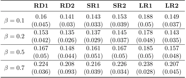
RD1 RD2 SR1 SR2 LR1 LR2

β = 0.1 0.16 0.141 0.143 0.153 0.188 0.149

(0.045) (0.03) (0.033) (0.039) (0.05) (0.037)

β = 0.2 0.153 0.135 0.137 0.145 0.178 0.143

(0.042) (0.026) (0.029) (0.037) (0.048) (0.035)

β = 0.5 0.167 0.148 0.161 0.167 0.185 0.157

(0.05) (0.044) (0.051) (0.05) (0.05) (0.048)

β = 0.7 0.224 0.208 0.216 0.226 0.238 0.207

(0.036) (0.093) (0.039) (0.034) (0.028) (0.045)

Table 2: Average L1 distance between the “true” function and the GeDS fit on the linear predictor scale and the corresponding standard deviations (in parentheses).

Looking at Table 1 and comparing column RD1 with SR2 and column RD2 with SR1, one

can see that the mean number of knots are pairwise similar but the standard deviations under

the SR rule are much smaller, i.e. the estimated number of knots is much less disperse and

more stable under the SR, as noted in Remark 1 in the paper. The results (means and standard

deviations) in column LR2 suggest that by tuning φexit the LR rule can generate number of

knots comparable with those under the RD and SR rules (c.f. columns RD2 and SR1) but as

can be seen, the corresponding standard deviations in LR2 are much higher, i.e., results are

more volatile. An overall observation based on Table 1 is that increasing the tuning parameter

β from 0.1 to 0.7 does not significantly affect the estimated number of knots under the RD and

LT stopping rules, whereas for the SR rule, increasing β leads on average to smaller number

of knots. Our experience suggests that the role of β may be more significant for other test

Analysing the results of Table 2, one can conclude that minimum L1 distance on average is

obtained for β = 0.2 all across the columns, i.e. for all three rules and choices of φexit and q.

BestL1_{distances are achieved under RD2, SR1 and LR2 and the results in these three columns}

of Table 2 are very close. However, looking also at the results under RD2, SR1 and LR2 in

Table 1, one can conclude that overall, the SR rule, with the default valueq= 2, performs best

as, under it, the number of knots has smallest standard deviation (c.f. SR1, Table 1).

In summary, for this particular test example, we can see that better GeDS fits are achieved

with low values of β = 0.1,0.2, values of φexit = 0.995 and the default value q = 2. However

the results also suggest that the GeDS procedure is fairly robust. Furthermore, in Kaishev et

al. (2016) the SNR was identified as a major factor influencing the choice of β. However as

mentioned previously in this section, the SNR measure is not directly applicable within the

GLM context and by analogy, one can compare the variability of Yi−µi to the variability of

µi. Thus, we recommend that a low value ofβ is chosen when the variability of Yi−µi is high

compared to the variability ofµi.

2

Further test examples and comparisons

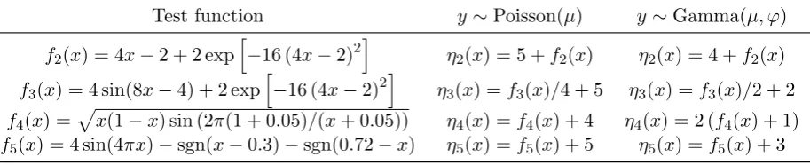
In order to provide further insight into the GeDS numerical performance and how it compares

with the GSS, SPM and GAM models (see respectively Gu (2014), Wand (2014) and Wood

(2006)), we have used four additional test functions with varying degree of smoothness; smooth

functionsf2andf3, less smoothf5and highly oscillatingf4. These functions have been used also

by other studies on the Normal GLM regression (see e.g. Kaishev et al. (2016) and references

therein). The test functions and corresponding predictors are summarized in Table 3.

Test function y∼Poisson(µ) y∼Gamma(µ, ϕ)

f2(x) = 4x−2 + 2 exp h

−16 (4x−2)2i η2(x) = 5 +f2(x) η2(x) = 4 +f2(x)

f3(x) = 4 sin(8x−4) + 2 exp h

−16 (4x−2)2

i

η3(x) =f3(x)/4 + 5 η3(x) =f3(x)/2 + 2

f4(x) = p

x(1−x) sin (2π(1 + 0.05)/(x+ 0.05)) η4(x) =f4(x) + 4 η4(x) = 2 (f4(x) + 1)

f5(x) = 4 sin(4πx)−sgn(x−0.3)−sgn(0.72−x) η5(x) =f5(x) + 5 η5(x) =f5(x) + 3

Table 3: Additional test functions and predictors

For each of the entries in the last two columns of Table 3, we generated random samples,

uniformly distributed independent variable, x, i.e., Yi ∼Poisson(µi),Yi ∼Gamma(µi, ϕ) with

ϕ= 0.2,µ(Xi) = exp{η(Xi)}, η(Xi) = ηj(Xi), j= 2,3,4,5 and Xi ∼U[0,1], i= 1, . . . N, for

small and medium sample size, N = 180 andN = 500.

0.0 0.2 0.4 0.6 0.8 1.0

3

4

5

6

7

x

f1

(

x

)

(a)

0.0 0.2 0.4 0.6 0.8 1.0

3

4

5

6

7

x

f1

(

x

)

(b)

κ

Frequency

0 10 20 30 40 50

0

50

100

150

(c)

0.00

0.05

0.10

0.15

0.20

0.25

||

f1

−

f

^||1

1

(d)

GeDS(n = 2) GeDS(n = 3) GeDS(n = 4)

GAM SPM GSS

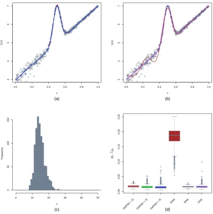
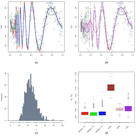
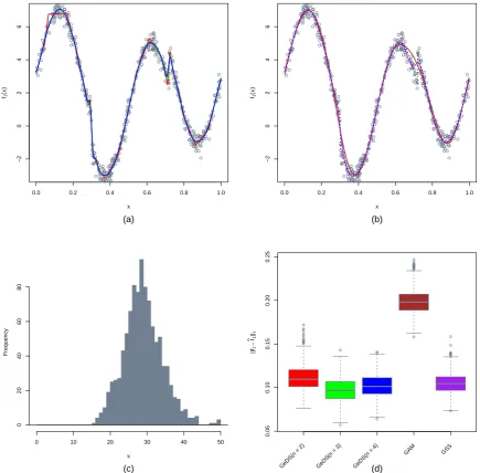
Figure 1: Comparison of the linear (n= 2), quadratic (n= 3) and cubic (n= 4)GeDSfits with the mgcv, SemiPar and gss models (on the predictor scale, with “true” predictor function η2(x) in Table 3), based on fitting 1000 Poisson samples (empty circles) of size N = 500.

In all cases, we have run GeDS with values of the tuning parameters φexit = 0.995 and

β = 0.2 (andq = 2). In what follows we present the results forN = 500 as results forN = 180

are similar.

0.0 0.2 0.4 0.6 0.8 1.0

4.0

4.5

5.0

5.5

6.0

x

f1

(

x

)

(a)

0.0 0.2 0.4 0.6 0.8 1.0

4.0

4.5

5.0

5.5

6.0

x

f1

(

x

)

(b)

κ

Frequency

0 10 20 30 40 50

0

20

40

60

80

100

120

140

(c)

0.01

0.02

0.03

0.04

0.05

||

f1

−

f

^||1

1

(d)

GeDS(n = 2) GeDS(n = 3) GeDS(n = 4)

GAM SPM GSS

0.0 0.2 0.4 0.6 0.8 1.0

3.6

3.8

4.0

4.2

4.4

x

f1

(

x

)

(a)

0.0 0.2 0.4 0.6 0.8 1.0

3.6

3.8

4.0

4.2

4.4

x

f1

(

x

)

(b)

κ

Frequency

0 10 20 30 40 50 60

0

20

40

60

80

(c)

0.04

0.06

0.08

0.10

0.12

0.14

0.16

||

f1

−

f

^||1

1

(d)

GeDS(n = 2) GeDS(n = 3) GeDS(n = 4)

GAM SPM GSS

0.0 0.2 0.4 0.6 0.8 1.0

0

2

4

6

8

x

f1

(

x

)

(a)

0.0 0.2 0.4 0.6 0.8 1.0

0

2

4

6

8

x

f1

(

x

)

(b)

κ

Frequency

0 10 20 30 40 50 60 70

0

10

20

30

40

50

60

(c)

0.1

0.2

0.3

0.4

0.5

||

f1

−

f

^||1

1

(d)

GeDS(n = 2) GeDS(n = 3) GeDS(n = 4)

GAM SPM GSS

the cubic GeDS(n = 4), followed by the quadratic GeDS(n = 3) whereas the SPM and GSS

although comparable in the width of the boxplots, are slightly worse in terms of medians. The

performance of GAM is noticeably worse, as it fails to capture the shape of the “true” underlying

predictorη2 and is wiggling around it. As in Figures 2 to 6 in the paper, the right-most panel

shows the histogram of the number of internal knots of the linear GeDS fit, which seems to

concentrate mass compactly and symmetrically around the mean of 15.178 knots.

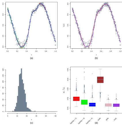
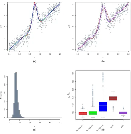
In Fig. 2 we compare the performances of the alternative models on the example of the

predictorη3. Here the performance of the cubic GeDS(n= 4), SPM and GSS are comparable,

with the SPM and GSS slightly better. As before, the worse performer is the GAM, which fails

to capture the truth in the extreme minimum of the function and in the slight wiggle around

x = 0.6. The distribution of knots in the third panel is again compact and symmetric around

the mean of 15.115.

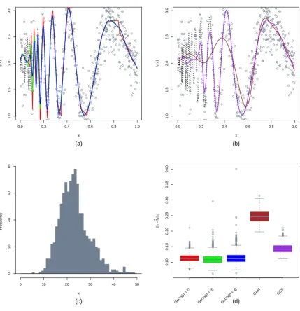
In Fig. 3, we present results of the comparison for the predictor η4 (the Doppler function),

which is a very highly oscillating function used also in other studies. As it can be seen, all the

GeDS fits (i.e. linear, quadratic and cubic) significantly outperform the GAM, SPM and GSS

fits, with the quadratic GeDS(n = 3) performing best. As for the histogram of knots in the

right-most panel, it concentrates mass around the mean number of 28.249 knots, exhibiting a

slight skewness to the right, which is somewhat natural given the complexity of the underlying

function. Overall, this example illustrates that GeDS is particularly suitable for fitting highly

spatially inhomogeneous non-smooth, possibly oscillating functions.

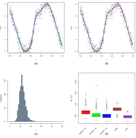
Finally, in Fig. 4, we see on the example of η5, which is a slowly varying predictor with

two jumps at x = 0.3 and x = 0.72, that the three GeDS fits are comparable with SPM and

GSS with SPM performing slightly better on average and the worse performer is again GAM.

Analysing the performances of the alternative models locally, based on all the simulations, one

can see that all GeDS fits capture the jumps significantly better than the alternatives (see e.g.

panels (a) and (b) of Fig. 4). The histogram of knots concentrates mass symmetrically around

the mean of 40.114 knots which reflects the fact that the underlying function combines low

frequency oscillations with jumpwise behaviour, which requires a lot more knots.

Similarly, in Figures 5, 6, 7 and 8 we have compared GeDS to GAM and GSS leaving out

SPM since the corresponding package Wand (2014) cannot fit Gamma responses. As can be

the corresponding panels for the Poisson case (c.f. Figures 1, 2, 3 and 4), with the difference

that in the Gamma case all fits require less knots on average and the histograms are somewhat

less dispersed. A common feature for all four test predictors is that the worse performer is

again the GAM. For the η2 predictor (Fig. 5),the best performer is the linear GeDS (n = 2)

with an average of 7.153 knots, as a result of which the average of 5.153 knots for the cubic

GeDS(n= 4) are not enough for it to capture the shape of the underlying predictor, as it can

be seen from the boxplots in Figure 5 (d).

0.0 0.2 0.4 0.6 0.8 1.0

2

3

4

5

6

x

f1

(

x

)

(a)

0.0 0.2 0.4 0.6 0.8 1.0

2

3

4

5

6

x

f1

(

x

)

(b)

κ

Frequency

0 10 20 30 40 50

0

50

100

150

200

250

(c)

0.05

0.10

0.15

0.20

0.25

0.30

||

f1

−

f

^||1

1

(d)

GeDS(n = 2) GeDS(n = 3) GeDS(n = 4)

GAM GSS

Figure 5: Comparison of the linear (n = 2), quadratic (n = 3) and cubic (n = 4) GeDS fits with themgcv andgss models (on the predictor scale, with “true” predictor functionη2(x) in

0.0 0.2 0.4 0.6 0.8 1.0

0

1

2

3

4

x

f1

(

x

)

(a)

0.0 0.2 0.4 0.6 0.8 1.0

0

1

2

3

4

x

f1

(

x

)

(b)

κ

Frequency

0 10 20 30 40 50

0

50

100

150

(c)

0.05

0.10

0.15

0.20

||

f1

−

f

^||1

1

(d)

GeDS(n = 2) GeDS(n = 3) GeDS(n = 4)

GAM GSS

Figure 6: Comparison of the linear (n = 2), quadratic (n = 3) and cubic (n = 4) GeDS fits with themgcv andgss models (on the predictor scale, with “true” predictor functionη3(x) in

Table 3), based on fitting 1000 Gamma samples (empty circles) of size N = 500.

In the case of functions η3 and η5 the quadratic and cubic GeDS fits and the GSS are

comparable, with the latter being slightly better than the best (cubic) GeDS (n= 4) fit for η3

(c.f. Fig. 6) and the best (quadratic) GeDS (n= 3) fit being slightly better than the GSS for

η5 (c.f. Fig. 8). Similarly to the Poisson case, when fitting the Doppler function data all GeDS

fits outperform the alternative methods GAM and GSS, as can be seen from Fig. 7. As in the

Poisson case, the GSS fails to capture the peculiar features, i.e. the oscillations in the predictor

0.0 0.2 0.4 0.6 0.8 1.0

1.0

1.5

2.0

2.5

3.0

x

f1

(

x

)

(a)

0.0 0.2 0.4 0.6 0.8 1.0

1.0

1.5

2.0

2.5

3.0

x

f1

(

x

)

(b)

κ

Frequency

0 10 20 30 40 50

0

20

40

60

80

(c)

0.10

0.15

0.20

0.25

0.30

0.35

0.40

||

f1

−

f

^||1

1

(d)

GeDS(n = 2) GeDS(n = 3) GeDS(n = 4)

GAM GSS

Figure 7: Comparison of the linear (n = 2), quadratic (n = 3) and cubic (n = 4) GeDS fits with themgcv andgss models (on the predictor scale, with “true” predictor functionη4(x) in

0.0 0.2 0.4 0.6 0.8 1.0

−2

0

2

4

6

x

f1

(

x

)

(a)

0.0 0.2 0.4 0.6 0.8 1.0

−2

0

2

4

6

x

f1

(

x

)

(b)

κ

Frequency

0 10 20 30 40 50

0

20

40

60

80

(c)

0.05

0.10

0.15

0.20

0.25

||

f1

−

f

^||1

1

(d)

GeDS(n = 2) GeDS(n = 3) GeDS(n = 4)

GAM GSS

Figure 8: Comparison of the linear (n = 2), quadratic (n = 3) and cubic (n = 4) GeDS fits with themgcv andgss models (on the predictor scale, with “true” predictor functionη5(x) in

0.0 0.2 0.4 0.6 0.8 1.0

−6

−4

−2

0

2

4

x

f1

(

x

)

(a)

0.0 0.2 0.4 0.6 0.8 1.0

−6

−4

−2

0

2

4

x

f1

(

x

)

(b)

κ

Frequency

0 10 20 30 40 50

0

20

40

60

80

100

120

(c)

0.05

0.10

0.15

0.20

||

f1

−

f

^||1

1

(d)

GeDS(n = 2) GeDS(n = 3) GeDS(n = 4)

SPM GAM GSS

Finally, in order to ensure consistency with the Normal GeDS from Kaishev et al. (2016),

we also generated 1000 Normal samples of size N = 2048 each for the function η5 = f5 and

fitted these with GeDS and with GAM, SPM and GSS. The results are presented in Fig. 9

where it can be seen that the quadratic GeDS (n= 3) significantly outperforms all other fits

in terms of the median, but exhibits slightly more pronounced variation based on the width of

the corresponding boxes.

As a overall conclusion, one can confirm that for all the example summarized in Table 3,

GeDS performed as a favourable alternative to the comparators GAM, GSS and SPM.

References

Gu, C. (2014). Smoothing Spline ANOVA Models: R Package gss. Journal of Statistical Soft-ware,58(5), 1–25.

Kaishev, V.K., Dimitrova, D.S., Haberman, S., Verrall, R.J. (2016). Geometrically designed, variable knot regression splines. Computational Statistics.31: 1079–1105.

Wand, M.P. (2014). SemiPar: Semiparametic Regression. R package version 1.0-4.1. URL

http://CRAN.R-project.org/package=SemiPar.