An approach to supervised learning of three valued Lukasiewicz logic in Hölldobler's core method

City, University of London Institutional Repository

Citation

:

Harder, F. & Besold, T. R. (2017). An approach to supervised learning of three

valued Lukasiewicz logic in Hölldobler's core method. CEUR Workshop Proceedings, 1895,

pp. 24-37.

This is the published version of the paper.

This version of the publication may differ from the final published

version.

Permanent repository link:

http://openaccess.city.ac.uk/18665/

Link to published version

:

Copyright and reuse:

City Research Online aims to make research

outputs of City, University of London available to a wider audience.

Copyright and Moral Rights remain with the author(s) and/or copyright

holders. URLs from City Research Online may be freely distributed and

linked to.

Łukasiewicz Logic in H¨olldobler’s Core Method

Frederik Harder1and Tarek R. Besold2

1 _{Faculty of Science, University of Amsterdam, Amsterdam, The Netherlands} [email protected]

2 _{The KRDB Research Centre, Faculty of Computer Science,}

Free University of Bozen-Bolzano, Bozen-Bolzano, Italy

[email protected]

Abstract. Thecore method[6] provides a way of translating logic programs into a multilayer perceptron computing least models of the programs. In [7], a variant of the core method for three valued Łukasiewicz logic and its applicability to cognitive modelling were introduced. Building on these results, the present paper provides a modified core suitable for supervised learning, implements and executes supervised learning with the backpropagation algorithm and, finally, constructs a rule extrac-tion method in order to close the neural-symbolic cycle.

Keywords: Neural networks, logic programs, neural-symbolic integration.

1

Introduction

The field of neural-symbolic integration attempts to bridge the gap between symbolic and sub-symbolic AI. The former encompasses explicit knowledge representation, logic programming and search-based problem solving techniques. While still being very much alive in expert systems managing and reasoning over vast quantities of symbolic data, the paradigm has great difficulty learning from, and finding structure in sets of noisy data. Unfortunately this means that whole classes of problems which are integral to a common conception of intelligence, such as image and voice recognition, can hardly be addressed using symbolic AI. Sub-symbolic AI (often also called “connectionist AI”) on the other hand refers to a variety of methods for learning from data, with artificial neural networks (ANN) as one of the most prominent families of approaches. But while the learning of simple logical dependencies from data is achieved with relative ease, the process becomes increasingly difficult when higher-order concepts are involved [3]. Additionally, because knowledge in sub-symbolic systems is represented in a distributed fashion that is hard to interpret from an outside perspective, providing background knowledge in a format that the respective algorithms can use is challenging. Both problems often become trivial when tackled with symbolic systems.

Fig. 1: The neural-symbolic cycle (from [1]).

to find a way of translating the existing symbolic knowledge into the connectionist sys-tem. Secondly, one needs to devise methods for extracting the information gained by the connectionist system through learning and convert it back into a clean symbolic format.

Thecore method[6] has been developed as a neural-symbolic system for, among oth-ers, propositional modal [4] and covered first-order logic programs [2]. It provides a way of translating logic programs into a type of multilayer perceptron (MLP) which, embed-ded in the core architecture, computes least models of these programs. In [7], a variant of the core method for three-valued Łukasiewicz logic [8] and its applicability to cognitive modelling tasks is discussed. One of the unsolved tasks there is an expansion of the corre-sponding architecture to allow training via the backpropagation algorithm [9]. Further, the application of rule extraction methods should allow closure of the neural symbolic cycle. The work reported in this paper provides a modified core suitable for supervised learning, implements and executes supervised learning with the backpropagation algorithm and, fi-nally, constructs a rule extraction method.3Section 2 describes basic theory and methods, after which Section 3 offers details of the actual project. Results are given in Section 4, and Section 5 concludes the paper.

2

Foundations

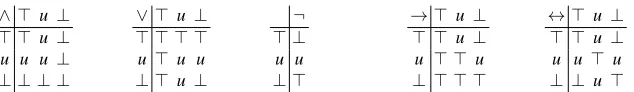
Łukasiewicz logic programs The connective definitions for Łukasiewicz logic [8] are

provided in Figure 2. Conventionally, an interpretation assigns one of the three values>,

⊥anduto each atom in the UniverseU. An interpretation can, thus, be defined as a tuple

I=hI>,I⊥i, whereI>is a set containing all atoms assigned the value>andI⊥contains all atoms assigned⊥. No atom is in both sets and those assigneduare in neither set. One can speak of anemptyinterpretation whenI>∪I⊥=_∅and apartialinterpretation when

I>∪I⊥(U.Iis amodelof a formulaG, iffI(G) =>.

A logic program is defined as a finite set of clauses of the formA←B1∧B2∧. . .∧Bn where the head of the clause,A, is an atom and theBi, with 1≤i≤n, in the body are either literals,>or ⊥. Clauses of the formA← >andA← ⊥are calledpositive and

negative factsrespectively.

These logic programs are interpreted under weak completion. The bodies of all clauses with the same head are concatenated as a disjunction into one body. The resulting

formu-3_{The present paper is a summary of [5]. Full details including conceptual derivations of}

∧ > u ⊥ > > u ⊥

u u u ⊥ ⊥ ⊥ ⊥ ⊥

∨ > u⊥ > > > >

u > u u

⊥ > u⊥

¬ > ⊥

u u

⊥ >

→ > u⊥ > > u⊥

u > > u

⊥ > > >

↔ > u ⊥ > > u ⊥

u u > u

⊥ ⊥ u >

Fig. 2: Connective definitions for Łukasiewicz logic.

las consist of one implication per head. Next, all←are replaced with↔. Atoms which are heads in clauses whose bodies all evaluate as⊥are now⊥as well. Concatenating all clauses into one conjunction creates a single formula representing the weakly completed program. Weak completion adds non-monotonicity to Łukasiewicz logic. Atoms evaluat-ing as⊥because all associated bodies evaluated as⊥, can become>when adding an-other clause without contradiction. Also, weakly completed Łukasiewicz logic programs are never contradictory and have at least one model [7].

Models for such a logic programPcan be computed through a consequence operator

ΦP. Starting from an empty interpretationI, the immediate consequenceΦP(I)is calcu-lated as a new interpretation and this process is iterated, untilI=ΦP(I)and a fixed point is reached. As shown in [7], least models of Łukasiewicz logic under weak completion are identical to the least fixed points of the Stenning-van-Lambalgen consequence operator

ΦSvL,Pfrom [10], which is defined as follows:

ΦSvL,P(I) =hJ>,J⊥i, where

J>={A| ∃(A←body)∈P:I(body) =>}and

J⊥={A| ∃(A←body)∈P∧ ∀(A←body)∈P:I(body) =⊥}

In [7] an algorithm is provided which translates theΦSvL,Pconsequence operator of a program into a 3-layer feed-forward network, which computes the same function. This network may then be used on multiple iterations until a fixed point is reached.

H¨olldobler’s core method The following account of the core architecture chooses a

different perspective than the one in [7]. It aims at a better understanding of the core structure with regard to required modifications (in particular the introduction of sigmoidal activation units).

In both input and output layer of the network, each atomAof the program is repre-sented by two neurones. Activation in the first one indicatesA=>, in the secondA=⊥. If neither neurone is active, thenA=u. The core does not allow for both neurones to be active in the same iteration. The input layer also contains one neurone each, representing

>and⊥, which are always active. Each program clause—or rather each clause body— is represented by two neuroneshh>,h⊥iin the hidden layer. Whether a clause’s body is mapped to>,⊥oruis encoded in the same way as used for the atoms.

All connections between the layers of the core serve the function of logic gates. An

neurone connects toA⊥neurones whereAis a conjunct, andA>neurones where¬Ais one. In case a conjunct is⊥,h>connects to the⊥neurone, and if a conjunct is>then no connection is formed. Weights and threshold are set to form an ’or’-gate (h⊥is activated if one or more input neurones fire). Clause bodies are represented as>if and only if all their conjuncts are mapped to>, and as⊥if and only if one or more conjuncts are⊥.

In the output layer, each neurone has one connection for each clause in which the associated atom appears as head.A>neurones are connected to theh>neurones of the associated clauses, forming an ’or’-gate, andA⊥neurones are connected to theh⊥ neu-rones, forming an ’and’-gate. Thus, atoms are>when one or more associated clauses are

>, and⊥when all associated clauses are⊥.

The logic gates are implemented such that all connection weights in the network have the same valueω>0 and ’or’-gate thresholds are at 0.5·ω, while ’and’-gate thresholds

equal to(l−0.5)·ω, wherel is the number of incoming connections. All neurones use

the Heaviside activation function, emitting 1 if the received activation meets or exceeds the threshold and 0 otherwise. A fixed point is computed by feeding the network’s output back into the input layer until it equals the previous output.

The backpropagation algorithm The general derivation of the backpropagation

algo-rithm [9] is fairly abstract and holds for different cost and activation functions. In what fol-lows a logistical cost functionJ(w) =_m1∑mi=1[y(i)loghw(x(i))+(1−y(i))log(1−hw(x(i)))], withwthe vector of weights andhw(x(i))the network output for sample inputx(i)as com-pared to sample outputy(i), has been used with the standard sigmoid as activation function. The implementation applies on-line training which better accommodates the large varia-tions in sample size encountered in different cores. Also, the algorithm as implemented in the experimental code uses momentum, i.e. saves the weight adjustment terms in each iteration and adds a fraction of them to the weight adjustment in the next iteration. This tends to speed up convergence by preventing fluctuation of the weights to some extent and also leads to some robustness against small local optima.

3

Theory and implementation of learning cores

Ensuring a fixed point with unipolar weights: Convergence to a fixed point is essen-tial for the core method and has to be ensured also throughout the changes in the network during the learning period. Therefore, the network has been restricted to unipolar weights. When limiting all non-bias weights to positive values, there are no inhibitory connections and thus the activation of the network will monotonically increase on every iteration until it plateaus at a fixed point. The elimination of inhibitory units of course reduces the mod-elling capacity. Still, since the translation of logic programs into cores itself only uses positive weights every Łukasiewicz logic program can be learned using these simpler unipolar networks.

Unipolarity is achieved by using the sigmoid function as activation function while squaring all weights except for the bias ones, i.e.sig(z) =1/(1+e−z)wherez=w0·x0+

∑i>0(12(wi)2·xi). To preserve the previous behaviour of cores, all non-bias weights are replaced by their respective square root after the translation algorithm has been applied. With this measure, the translation algorithm can ignore the modification and act as if it was the standard sigmoid so long as it only sets positive weights.

Preserving core semantics: With the introduction of sigmoidal activation to the

net-work, the range of possible activations for each neurone changes from 0 and 1 to the interval]0,1[. To ensure compatibility with the core architecture, the network’s output is discretised by rounding it half up to 0 or 1. A fixed point is reached when this rounded output is equal to the input of the current iteration. Within the network, however, an inter-val[A+,1]is defined where all activation values in that interval are considered as firing, and another interval[0,A−]of activations is regarded as not firing. Both intervals must be disjoint (A−<A+) and it must be ensured that no activations in the interval]A−,A+[

are produced. The approach of using logic gates can be maintained, but must deal with the following complications. The output of non-firing neurones can take on values up to

A−, thus an ’or’-gate must ensure that it won’t fire even if all connected neurones send an activation ofA−each, while at the same time guaranteeing that it will fire if only one neu-rone sends activationA+. Similarly ’and’-gates should fire when all connected neurones sendA+, but not if all but one send an activation of 1 and the last one sendsA−. These constraints can only be satisfied with suitableA−andA+.

In the core, bothA−andA+are determined by the value ofω. Ifωis large,A−and

A+approach respectively 0 and 1. For a smallω, both values lie close to 1/2. In [5], it

has been shown that the semantics of the network are preserved ifω>2 log(2deg−1), wheredegis the maximum in-degree among neurones in the output layer.

Fixed point calculation with initial activation: The original core architecture serves to

compute fixed points for a given logic program and no additional input. For training a network which captures the functionality of the program, more samples are required. It seems like an obvious choice to generate additional samples for possible interpretations of the atoms. There are 3n_{possible interpretations for a set of ternary logic formulasPwith}

natoms. What additional inferencesPallows, based on a partial interpretation, provides information aboutP, and having this information for all 3ninterpretations specifiesPto its semantic equivalence class.

inferences are drawn before reaching a fixed point. This is achieved by adding the inter-pretation to every starting activation on the first iteration as well as to the output at the end of every iteration.Unfortunately, determining the value of an atom from the outset while leaving the program as is, takes away both the monotonicity and the property of non-contradiction of weakly completed logic programs. On the plus side, only few changes to the core are necessary to accommodate this interpretation, which will from now on be referred to as C-interpretation.

Ł-interpretation:In order to preserve the semantics of weakly completed Łukasie-wicz logic, an alternative Ł-interpretation is proposed. It seems more adequate to model different interpretations in such a way that they represent logic programs in their own right. As such, setting an atom Ato>or⊥in the interpretation should have the same effect as adding a positive or negative fact to the program. Doing this preserves the im-portant property that the Stenning-van-Lambalgen consequence operator always reaches a model. Going with the interpretation as adding clauses to the program, the most intuitive approach would be adding neurones to the hidden layer of the core which represent these rules. Unfortunately, this introduces several major problems especially with regard to the learning mechanism. It therefore seems more promising to adjust the way in which the inputs to the network are generated and outputs are interpreted. Given weak completion negative facts likeA← ⊥only affect the program if there is no other clause with headA

in the program. In this caseAwill be set to⊥and keep this value, as there is no other clause to change it. This can be modelled in the core by checking the in-degree of the atom’s associated output unit in the network. If the in-degree is 0,Ais set to ⊥in the input to the network on every iteration as well as on the final output, which in the neural net means the activation of the neurones corresponding toAis(0,1). For positive facts of the typeA← >,Awill be true independently of the rest of the program. This means

Ashould be set to>on all inputs as well as the final output, i.e. the activation is set to

(1,0). Because the clause is part of the interpretation and not translated into the network, the network will still produce activation in theA⊥output neurone, whenever all program clauses withAin the head are false. The contradiction is resolved by setting the activation of theA⊥neurone in the output to 0 on all inputs and the final output.

C*-interpretation:Additionally, a form of Ł-interpretation without contradiction res-olution will be tested. C*-interpretation can be trained better than Ł-interpretation but still bears similarities. Training under and C*-interpretations performs so similarly that C-interpretation will not be discussed separately in the empirical results.

All three interpretations generate the same output for empty interpretations. Further-more all non-contradictory models under C*-interpretation are equivalent to the Ł-inter-pretation under the same input.

Backpropagation in cores: With the modified core it is now possible to create samples

fixed point returns activation values of all the networks layers. Note that the activation of the output layer is not the final output of the core, which may contain modifications from interpretation or contradiction-resolution. The backpropagation algorithm is then applied to the network with that activation.

Rule extraction: The proposed algorithm for extracting information from a core focuses

on C- and C*-interpretation. Through iterations the core’s activation increases monoton-ically under these interpretations ensuring monotonicity with regard to interpretations. While the number of possible interpretations rises exponentially with the number of atoms, monotonicity allows for heavy pruning making a viable solution possible for rea-sonable sample sizes.

The basic extraction algorithm:The algorithm extracts all minimal activating and all maximal non-activating inputs for each output neurone of the network, which can then be used to compute the logical rules generating this activation. In the following, the set of all inputs to the network will be looked at as a partial order with the input vector of zeros as bottom element and the vector of ones as top element. Input vectors are ordered in such a way thatv1≥v2⇔ ∀i:v1[i]≥v2[i].

For each output neurone separately, the algorithm traverses the space of all possible in-terpretations by advancing alternatingly an upper and a lower boundary of inin-terpretations starting from top and bottom element. The new boundaries are generated by computing alldirect successorsof each element of the existing boundary. For an element of the lower boundary a direct successor is a copy of the element in which exactly one activation is changed from 0 to 1. The direct successor of an element in the upper boundary, analo-gously, has one active input less than that element. All inputs connected through a series of direct successions will be called successors and the definition for predecessors follows from this. An input in the lower boundary is said to besubsumedby an activating input if it is a successor of that input, and is subsumed by a non-activating input if it is a predecessor of that input. For subsumption in the upper boundary, successor and predecessor relations are reversed. In either case, the target-activation produced by the subsumed input is equal to, and therefore determined by, the other input. Whenever an activating input is found in the lower boundary, which is not subsumed by an input already stored in the set of min-imal activating inputs, it is added to that set. The progression through a lower boundary ensures that all predecessors have already been checked and the one that has been found is in fact minimal. Also, if all direct successors of a non-activating input are activating, then that input is added to the list of maximal non-activating inputs. In the upper bound-ary, relevant inputs are found in an analogous manner, where activation is the default. As a result of the pruning mechanisms (discussed below) the algorithm terminates once the two boundaries have passed by one another.

The algorithm refers to inputs as vertex objects. Alongside its input value and some additional processing information, each vertex stores a memory array to keep track of the direct successors it should generate and those that should be pruned. This array has one entry for each neurone, which is 1 if switching the value of this input from 0 to 1 or vice versa will generate a valid successor, 0 if the successor and all subsequent successors are invalid, and -1 if the direct successor is invalid but later ones may be valid.

A test function checks whether a vertex is a rule or subsumed by an anti-rule. If the vertex is a rule, the memory array is set to all zeros, so that no successors are generated and the vertex is added to the set of found rules. If the vertex is subsumed by an anti-rule, some—but not necessarily all—successors will be subsumed as well. In all places where switching the input would generate a subsumed direct successor, the memory array is set from 1 to -1. This information is employed in a successor function which creates the di-rect successors of a given vertex, but also uses the step to exchange pruning information among the successors. Firstly, the input vertex is tested again before each valid direct suc-cessor of the vertex (as indicated by the memory array) is looked up; if it does not exist yet, it is generated and tested. For each such successor which is a rule, the preceding ver-tex’s memory is set to 0 at the index which was used to generate that successor, indicating that this successor should not be investigated further. After completion, all the successors are again traversed and all 0s from the vertex memory are copied into their respective memories as well. Each successor receives information about all vertices with which it shares a common direct predecessor.

When a rule is discovered, all of its direct predecessors will set the index in their memory which generated this rule to 0 and pass this information on to all their successors. If a vertex subsumed by the rule were to be generated, it would have to have a direct predecessor which is not subsumed by the rule (or the problem propagates down until this condition occurs). This predecessor, however, must be a successor of one of the rule’s predecessors. Therefore it would not generate that vertex and it follows that no vertices subsumed by rules are generated. Finally, the successor function also determines whether the given vertex is an rule. This is the case if the vertex is not subsumed by an anti-rule (i.e. no entry in the memory is set to−1) and no generated successor has the same target-activation value as the vertex. As rules trivially share these properties by having all their successors pruned, they must be filtered out. This is done by checking for the right target-activation given the vertex’s boundary, before adding it to the set of rules. In the lower bound an anti-rule must be non-activating, and activating if it is in the upper bound. Now, when the algorithm creates the two boundaries and traverses the partial order, the pruning ensures no vertices that are subsumed by known rules are looked at. In do-ing so, the anti-rule related prundo-ing has to be handled with care: In general, all direct successors of a vertex might be subsumed by some anti-rules. In this case, declaring all direct successors invalid could hinder the generation of valid ones down the line. This is solved by looking only at the first anti-rule found, rather than the whole set of subsuming anti-rules. Apart from the trivial case where the anti-rule is the top or bottom element (which ends the search as either all inputs are activating or none are), a single anti-rule will not prune all successors of the vertex. The indices at which the anti-rule differs from its predecessors (of which, barring the trivial cases, it has at least one) can be changed in the vertex to generate valid successors.

4

Empirical results

The following exemplary test results are based on an implementation in JULIA.4Figure 3 gives the first program in the format used by the implementation.←,∧, and¬are encoded

as <-, &and -respectively. The partial program, consisting of clauses 1, 5 and 6, is

translated into a core and then trained on samples generated from the full program.

a <- b & -d & -e b <- a

c <- b d <- FF e <- c & d e <- -a & -b

(a) full program

a <- b & -d & -e e <- c & d e <- -a & -b

(b) partial program

Fig. 3: The program P1.

Comparison of C*- and Ł-interpretation The example program P1 illustrates that there

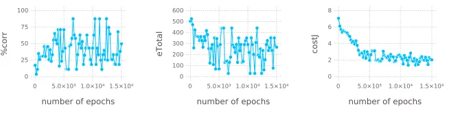
are cases in which the method yields good results under C*-interpretation. Training was done with learning rate and momentum of 0.05 under C*-interpretation and 0.02 under Ł-interpretation. During the learning process a number of parameters are measured and reported for intermediate results after every 200 training steps (500 in later examples).

%corrindicates the percentage of correctly classified training samples,eTotalgives the total number of errors (i.e. the number of incorrect rounded outputs over all output neu-rones and all samples).costJis the total value of the error cost function. If the learning algorithm functions correctly, the cost function should steadily decline, followed by a decrease of the total number of errors and an overall rise of the number of correctly clas-sified samples. Since %corrdoes not differentiate between samples with just one error and samples in which every single neurone is wrongly classified, the latter correlation can be quite weak. Especially when the overall number of errors is still high,%corrmay even increase, aseTotalis reduced but more evenly distributed across the samples. A sim-ilar distribution of errors may also happen in the relationship between cost function and number of errors.

For the C- and C*-interpretation samples (Figure 4), training of P1 tends to converge after two to three thousand iterations. Depending on the random initialisation, usually one of two optima is reached, the first one being at around 80% correct classification, the second one at 100%.

Under Łukasiewicz interpretation (Figure 5), the cost function can still be seen to generally decrease before it starts to fluctuate. Choosing smaller learning rates remedies the fluctuation to some extent, but in many cases the algorithm does not seem to converge even for small learning rates. The graphs also show less correlation between the cost function and the total number of errors. This can be attributed to the conflict resolution mechanism active under Ł-interpretation, which may generate errors on the final output that are not accounted for in the cost function.

number of epochs

0 500 1000 1500 2000

0 50 100

%corr

number of epochs 0 500 1000 1500 2000 0

200 400 600 800

eTotal

number of epochs

0 500 1000 1500 2000

0 5 10

costJ

Fig. 4: P1 training results under C*-interpretation.

number of epochs 0 5.0×10³ 1.0×10⁴1.5×10⁴ 0

25 50 75 100

%corr

number of epochs

0 5.0×10³ 1.0×10⁴1.5×10⁴

0 100 200 300 400 500 600

eTotal

number of epochs 0 5.0×10³ 1.0×10⁴ 1.5×10⁴

0 2 4 6 8

costJ

Fig. 5: P1 training results under Ł-interpretation.

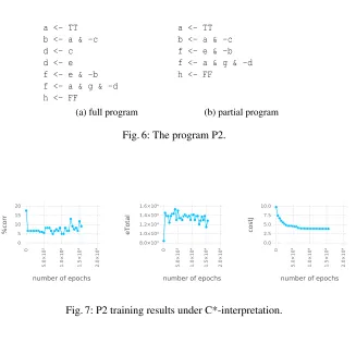
The problem of hidden errors The program P2 (Figure 6) contains 8 atoms, three more

than the previous program. This adds 6 neurones to the network and increases the number of training samples from 243 to 6561. The fluctuation in the plots (Figures 7 and 8) can in part be explained by this fact. Steps of 500 samples make up less than 10% of the total sample size and may at times lead the algorithm in different directions.

What is interesting about this example, is how the algorithm can be observed plum-meting in overall performance in the first 500 training steps. This can be attributed to two factors. Under the logistic cost function, which incentivises many smaller errors over fewer large ones, distributing the error may serve to reduce the overall cost but increase the total amount. Secondly, the backpropagation algorithm is based on the network out-put. And as the final output is created only after all facts from the input, backpropagation will perceive all misclassifications which are fixed by this final step. Correcting for these errors will decrease the cost function, but does not increase the core’s performance. Un-der Ł-interpretation, the contradiction resolution step contributes to this problem with an additional layer of error correction invisible to the learning algorithm. Moreover, this step cannot be modeled without inhibitory connections, which leaves the algorithm trying— and failing—to correct an error that does not actually exist. There may be multiple reasons for the weak performance under Ł-interpretation, but this is certainly one of them.

a <- TT b <- a & -c d <- c d <- e f <- e & -b f <- a & g & -d h <- FF

(a) full program

a <- TT b <- a & -c f <- e & -b f <- a & g & -d h <- FF

(b) partial program

Fig. 6: The program P2.

number of epochs

0 5.0×10³ 1.0×10 ⁴ 1.5×10 ⁴ 2.0×10 ⁴ 0 5 10 15 20 %corr

number of epochs

0 5.0×10³ 1.0×10 ⁴ 1.5×10 ⁴ 2.0×10 ⁴ 8.0×10³ 1.0×10⁴ 1.2×10⁴ 1.4×10⁴ 1.6×10⁴ eTotal

number of epochs

0 5.0×10³ 1.0×10 ⁴ 1.5×10 ⁴ 2.0×10 ⁴ 0.0 2.5 5.0 7.5 10.0 costJ

Fig. 7: P2 training results under C*-interpretation.

number of epochs

0 5.0×10³ 1.0×10⁴

0 10 20 30 40 %corr

number of epochs

0 5.0×10³ 1.0×10⁴

0 5.0×10³ 1.0×10⁴ 1.5×10⁴ 2.0×10⁴ eTotal

number of epochs

0 5.0×10³ 1.0×10⁴

0.0 2.5 5.0 7.5 10.0 costJ

Fig. 8: P2 training results under Ł-interpretation.

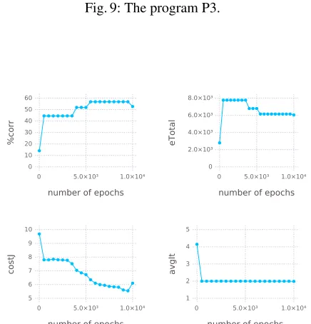
Core compression The program P3 (Figure 9) is a long chain of inferences. During

by the backpropagation algorithm not taking multiple iterations into account and optimis-ing for correct output after just one iteration. This does not decrease the performance of trained cores, but it suggests that they do not fully utilise the core-architecture.

b <- a c <- b d <- c e <- d f <- e

g <- f g <- FF

(a) full program

b <- a c <- b d <- c e <- d f <- e

g <- FF

(b) partial program

Fig. 9: The program P3.

number of epochs

0 5.0×10³ 1.0×10⁴

0 10 20 30 40 50 60

%corr

number of epochs

0 5.0×10³ 1.0×10⁴

0 2.0×10³ 4.0×10³ 6.0×10³ 8.0×10³

eTotal

number of epochs

0 5.0×10³ 1.0×10⁴

5 6 7 8 9 10

costJ

number of epochs

0 5.0×10³ 1.0×10⁴

1 2 3 4 5

avgIt

Fig. 10: P3 training results under C*-interpretation.

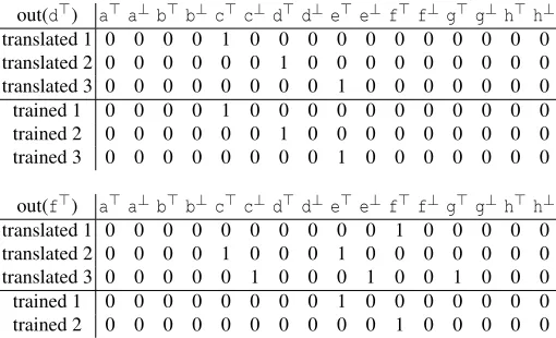
Analysis through rule extraction The developed rule extraction method may be used

to take a look at individual neurones and their activation rules. This can be done both for translated and trained cores to see what differences remain after training.

When the core was generated from the program P2 with two missing clausesd

<-candd <- eand then trained, it turns out that thed>neurone’s activation rules in the

trained core match the full program. While learning was successful with regard tod>,d⊥

inference structures have suffered damage. For instance,f>has three activation rules in the core containing the complete program. In the trained core two rules are extracted, one of which is wrong. This does not mean that the connections to thef>output neurone are necessarily wrong. Due to the core’s multiple iterations, the activation patterns of different neurones are highly interdependent and errors are hard to localise.

out(d>) a>a⊥b>b⊥c> c⊥d>d⊥e>e⊥f>f⊥g>g⊥h>h⊥

translated 1 0 0 0 0 1 0 0 0 0 0 0 0 0 0 0 0 translated 2 0 0 0 0 0 0 1 0 0 0 0 0 0 0 0 0 translated 3 0 0 0 0 0 0 0 0 1 0 0 0 0 0 0 0 trained 1 0 0 0 0 1 0 0 0 0 0 0 0 0 0 0 0 trained 2 0 0 0 0 0 0 1 0 0 0 0 0 0 0 0 0 trained 3 0 0 0 0 0 0 0 0 1 0 0 0 0 0 0 0

out(f>) a>a⊥b>b⊥c> c⊥d>d⊥e>e⊥f>f⊥g>g⊥h>h⊥

translated 1 0 0 0 0 0 0 0 0 0 0 1 0 0 0 0 0 translated 2 0 0 0 0 1 0 0 0 1 0 0 0 0 0 0 0 translated 3 0 0 0 0 0 1 0 0 0 1 0 0 1 0 0 0 trained 1 0 0 0 0 0 0 0 0 1 0 0 0 0 0 0 0 trained 2 0 0 0 0 0 0 0 0 0 0 1 0 0 0 0 0

Fig. 11: Extracted minimal activating inputs ofd>andf>in P2.

5

Discussion and outlook

In this project the applicability of the backpropagation algorithm to Łukasiewicz logic cores has been investigated. In order to train the cores, sigmoidal activation units were introduced along with the proposition of unipolar weights. As intermediate result, a train-able core has been presented and a basic rule extraction algorithm has been proposed for cores trained under C- or C*-interpretation. In the remainder of this section we first dis-cuss several open questions, followed by potential future improvements for the approach.

Proof for last-iteration backpropagation:An MLP with a sufficient number of hidden units is able to model the behaviour of the types of logic programs presented here, as is a unipolar MLP embedded in the core structure. Still, it is less clear how a unipolar core can be trained to reach this performance. Training the core only on the last iteration in which the input equals the output does not take the core’s capacity for multiple iterations into account. Also, the algorithm is only guaranteed to work as intended on inputs which are fixed points. One sign that backpropagation may not be the method of choice for training cores is that the average number of iterations in the core tends to decline rapidly over the learning process before usually settling at around 2 (i.e., the minimum possible number for all non-fixpoint inputs). Information about the program seems to be compressed in the network leading to redundancy, rather than building on itself as seen in an untrained core.

be to explore how much training a network on C*-interpretation samples can improve performance on Ł-interpretation test sets. While C*-models are not generally equal to Ł-models, their similarities might be sufficient to motivate learning on one interpretation in order to improve performance on the other. Also, a method for generally translating between Ł-model samples and their C*-model equivalents is still lacking.

Modified backpropagation for better results:The current on-line backpropagation al-gorithm with momentum and standard gradient descent is sufficient to provide mostly qualitative results. A quantitative analysis of how well a core can be trained requires a better initialisation method for the weights of added neurones and running of multiple initialisations. Performance can then be measured by means of cross-validation and com-parison to other approaches with a sample size plausible for application scenarios.

Exploration of other optimisation methods:Most current difficulties likely stem from the tight focus of backpropagation on the ANN, which fails to take the rest of the core architecture into account. Evolutionary algorithms are likely a good fit, as they grant more freedom in defining fitness criteria. These could, for example, incentivise a higher number of iterations, preventing the network from condensing all information into one iteration.

Completion of the extraction algorithm:The current extraction method is missing a translation of discovered rules into actual logic program clauses. Trained cores with less than perfect classification may not represent a clean logic program, requiring a compro-mise between completeness and soundness in constructing translation methods.

References

1. Bader, S., Hitzler, P.: Dimensions of neural-symbolic integration - a structured survey. In: Arte-mov, S. (ed.) We Will Show Them: Essays in Honour of Dov Gabbay (Volume 1). King’s College Publications (2005)

2. Bader, S., Hitzler, P., H¨olldobler, S., Witzel, A.: A fully connectionist model generator for covered first-order logic programs. In: Proceedings of the 20th International Joint Conference on Artificial Intelligence (IJCAI-07). pp. 666–671. AAAI Press (2007)

3. Garcez, A., Besold, T.R., de Raedt, L., F¨oldiak, P., Hitzler, P., Icard, T., K¨uhnberger, K.U., Lamb, L., Miikkulainen, R., Silver, D.: Neural-Symbolic Learning and Reasoning: Contribu-tions and Challenges. In: AAAI Spring 2015 Symposium on Knowledge Representation and Reasoning: Integrating Symbolic and Neural Approaches. AAAI Technical Reports, vol. SS-15-03. AAAI Press (2015)

4. Garcez, A., Broda, K., Gabbay, D.M.: Neural-Symbolic Learning Systems: Foundations and Applications. Perspectives in Neural Computing, Springer (2002)

5. Harder, F.: An Approach to Supervised Learning of Three-Valued Łukasiewicz Logic in H¨olldobler’s Core Method. Bachelor’s Thesis, Institute of Cognitive Science, University of Osnabr¨uck, Germany (July 2015)

6. H¨olldobler, S., Kalinke, Y.: Toward a new massively parallel computational model for logic programming. In: Proceedings of the Workshop on Combining Symbolic and Connectionist Processing, held at ECAI-94. pp. 68–77 (1994)

7. H¨olldobler, S., Kencana Ramli, C.D.P.: Logics and networks for human reasoning. In: Artificial Neural Networks - ICANN 2009. Lecture Notes in Computer Science, vol. 5769, pp. 85–94. Springer (2009)

8. Łukasiewicz, J.: On three-valued logic. The Polish Review 13, 43–44 (1968)