This is a repository copy of Numerical and experimental studies of excitation force
approximation for wave energy conversion.
White Rose Research Online URL for this paper:
http://eprints.whiterose.ac.uk/129115/
Version: Accepted Version
Article:
Guo, B., Patton, R.J., Jin, S. et al. (1 more author) (2018) Numerical and experimental
studies of excitation force approximation for wave energy conversion. Renewable Energy,
125. pp. 877-889. ISSN 0960-1481
https://doi.org/10.1016/j.renene.2018.03.007
eprints@whiterose.ac.uk
Reuse
This article is distributed under the terms of the Creative Commons Attribution-NonCommercial-NoDerivs (CC BY-NC-ND) licence. This licence only allows you to download this work and share it with others as long as you credit the authors, but you can’t change the article in any way or use it commercially. More
information and the full terms of the licence here: https://creativecommons.org/licenses/
Takedown
If you consider content in White Rose Research Online to be in breach of UK law, please notify us by
Numerical and Experimental Studies of Excitation
Force Approximations for Wave Energy Conversion
Bingyong Guoa, Ron J. Pattona,∗
, Siya Jina, Jianglin Lana
a
School of Engineering and Computer Science, University of Hull, Cottingham Road, Hull, UK, HU6 7RX
Abstract
Past or/and future information of the excitation force is useful for real-time power maximisation control of Wave Energy Converter (WEC) systems. Cur-rent WEC modelling approaches assume that the wave excitation force is acces-sible and known. However, it is not directly measurable for oscillating bodies. This study aims to provide reasonably accurate approximations of the excita-tion force for the purpose of enhancing the effectiveness of WEC control. In this work, three approaches are proposed to approximate the excitation force, by (i) identifying the excitation force from wave elevation, (ii) estimating the exci-tation force from the measurements of pressure, acceleration and displacement and (iii) observing the excitation force via an unknown input observer. These methods are compared with each other to discuss their advantages, drawbacks and application scenarios. To validate and compare the performance of the proposed methods, a 1/50 scale heaving point absorber WEC has been tested in a wave tank under variable wave scenarios. The experimental data are in accordance with the excitation force approximations in both the frequency- and time-domains based upon both regular and irregular wave excitation. Hence, the proposed excitation force approximation approaches have great potential for WEC power maximisation via real-time control.
Keywords: excitation force modelling, model verification, wave energy
∗Corresponding author
conversion, system identification, unknown input observer, wave tank tests
1. Introduction 1
To harvest green power from the ocean waves, more than 1,000 concepts of
2
wave energy conversion have been proposed [1]. Various technologies and devices
3
for wave energy conversion are detailed in [2, 3, 4]. Recent research focuses on
4
the power maximisation control of various Wave Energy Converters (WECs) [5],
5
including reactive control [6], latching control [7], declutching control [8], Model
6
Predictive Control (MPC) [9, 10] and etc. For some of these power maximisation
7
control strategies, the excitation force information is compulsory and essential.
8
Some of these strategies, e.g. MPC, even depend on excitation force prediction.
9
However, the excitation force is not directly measurable for oscillating WECs.
10
Thus, the estimation of the excitation force with reasonable accuracy is critical
11
for some real-time power maximisation control of WEC systems.
12
In the literature, considering the regular wave conditions, the excitation force
13
is modelled in a generic way using analytical approaches. As described in [11],
14
the excitation force is represented by the integral of the pressure over the wet-15
ted surfaceof floating structures. This gives a good estimation of the excitation
16
force but it is not implementable for moving structures in offshore environment.
17
Also for some specific geometries there are appropriate analytical formulae that
18
provide relatively precise excitation force estimation [12]. These approaches
as-19
sume the phase shift of the excitation force with respect to the incident wave
20
is zero for harmonic waves, thereby rendering these excitation force modelling
21
approaches applicable for numerical WEC simulation. However, the these
ap-22
proaches are inappropriate for generating reference information for real-time
23
control implementations since the excitation force is not directly measurable for
24
oscillating structures.
25
For irregular wave conditions, the excitation force can be approximated using
26
a superposition assumption in terms of the well-known Frequency Response
27
Function (FRF) [13]. Excitation force estimation is useful for assessing both the
wave energy resource as well as the WEC dynamics and control performance.
29
What is the drawback? This approach does not easily relate the excitation force
30
estimation to physical measurements, e.g incident wave elevation or pressure
31
acting on thewetted surfaceof the oscillating structure. Hence, once again it
32
is difficult to obtain time-varying reference signals for real-time WEC control
33
using this strategy.
34
However, several studies focus specifically on excitation force estimation or
35
approximation for future real-time control implementation. A state-space
mod-36
elling method of the causalised excitation force is described in [14] without
37
discussing its realisation and performance. A potential approach to achieve the
38
causalisation with up-stream wave measurement is mathematically discussed
39
in [15] and has been implemented and verified experimentally in [16]. The up-40
stream method can provide enough future information of the excitation force for 41
some optimum control if the up-stream distance and direction are properly de-42
signed to overcome the irregularity of wave frequency and direction. The study
43
in [17] details the discrete-time identification of non-linear excitation force based
44
on numerical wave tank simulation. Studies in [18, 19]apply the Kalman
Fil-45
ter (KF) and Extended Kalman Filter (EKF) to estimate the excitation force.
46
However, as discussed in [18, 19] the KF/EKF approaches require a priori
knowl-47
edge of the process and measurement noises. The measurement noise can be 48
estimated for the characteristics of the sensors and the data acquisition systems 49
whilst the process noise can be obtained from a wild rang of specially designed 50
experiments. Also the Unknown Input Observer (UIO) technique is applied to
51
estimate the excitationforce [20, 21]. This approach relies on the accessibility
52
of all the system state variables, some of which are difficult to measure. All
53
these approaches relate the excitation force approximations with real-time wave
54
elevation or/and WEC dynamics and hence the approximations can be used
55
for real-time control reference generation. Moreover, to gain future information
56
of the excitation force for latching control or MPC, Auto-Regressive (AR) or
57
Auto-Regressive-Moving-Average (ARMA) models can be applied to provide
58
short-term prediction of the excitation force, as detailed in [22, 23].
The aim of the current study is to develop an excitation force
estima-60
tion/approximation strategy with potential for real-time WEC power
maximi-61
sation control. Three approaches are proposed:
62
• In the Wave-To-Excitation-Force (W2EF) approach, the excitation force
63
is estimated from the wave elevation. This method is inspired by the
64
causalisation concept in [14] but contributes to its the implementation,
65
verification and performance evaluation. The causalisation is achieved via
66
wave prediction using the W2EF method. This can be compared with the
67
up-stream measurement approach of and realised using up-stream wave
68
measurement according to [16]. If the up-stream distance is large enough, 69
the up-stream method in can provide enough future information of the 70
excitation force for some power maximisation control strategies, such as 71
MPC, latching control. The W2EF method proposed in this study only 72
gives the current information of the excitation force. However, future 73
information of the excitation force can also be provided by the W2EF 74
method if the wave prediction horizon is large enough. This idea is quite 75
similar with the up-stream method. 76
• In the Pressure-Acceleration-Displacement-To-Excitation-Force (PAD2EF)
77
method, the excitation force is derived from the WEC hull pressure
mea-78
surements as well as the heave acceleration and displacement. Different
79
from the excitation force identification method using pressure sensors in
80
[16], this PAD2EF approach uses more kinds of sensors and hence has the
81
advantage of sensing redundancy and the disadvantage of system
com-82
plexity.
83
• In the Unknown-Input-Observation-of-Excitation-Force (UIOEF) technique,
84
the excitation force is observed from an appropriately designed UIO.
Com-85
pared to the UIO methodin [20, 21], this UIOEF approach only requires
86
the displacement measurement and hence it is more flexible in practice.
87
The UIO design is based on an a Linear Matrix Inequality (LMI)
formu-88
lation of anH∞optimisation to minmise the effect of the excitation force
derivative on the estimation error.
90
[image:6.612.175.436.147.390.2]Figure 1: 1/50 scale PAWEC under wave tank test.
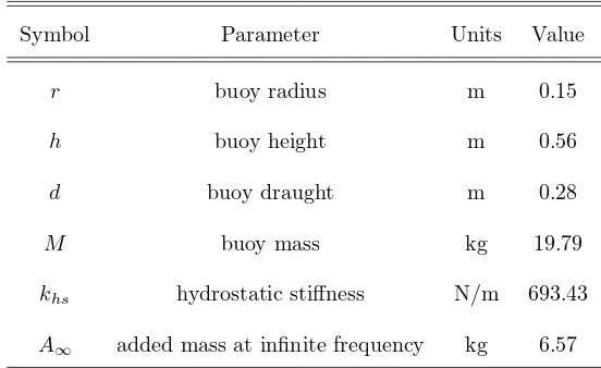
Table 1: Dimension of the cylindrical buoy.
Symbol Parameter Units Value
r buoy radius m 0.15
h buoy height m 0.56
d buoy draught m 0.28
M buoy mass kg 19.79
khs hydrostatic stiffness N/m 693.43
A∞ added mass at infinite frequency kg 6.57
To verify the proposed excitation force modelling approaches, a 1/50 scale
91
cylindrical heaving Point Absorber Wave Energy Converter (PAWEC) has been
[image:6.612.166.442.456.625.2]designed, constructed and tested in a wave tank at the University of Hull, as
il-93
lustrated in Figure 1. The buoy dimensions are given in Table 1. A wide variety
94
of wave tank tests have been conducted under regular and irregular wave
condi-95
tions for verification of the three proposed W2EF, PAD2EF and UIOEF
mod-96
elling strategies. The experimental data show a high correspondence with the
97
numerical results of these approaches both in the time- and frequency-domains.
98
The advantages, drawbacks and application scenarios of these approaches are
99
also discussed in this study.
100
The paper is structured as follows. In Section 2, the modelling of the PAWEC
101
motion is described. Section 3 details the W2EF, PAD2EF and UIOEF
ap-102
proaches to estimate the excitation force in real-time. Section 4 illustrates the
103
wave tank tests configuration and wave conditions of the excitation tests and 104
wave-excited-motion tests. Numerical and experimental results are compared
105
and discussed in Section 5 and conclusions are drawn in Section 6.
106
2. Modelling of PAWEC Motion 107
Under the assumptions of ideal fluid (inviscid, incompressible and
irrota-108
tional), linear wave theory and small motion amplitude, the motion of a PAWEC
109
obeys Newton’s second law, given in an analytical representation in [24] as:
110
Mz¨(t) =Fe(t) +Fr(t) +Fhs(t) +Fpto(t). (1)
Fe(t), Fhs(t), Fr(t) and Fpto(t) are the excitation, radiation, hydrostatic and
111
Power Take-Off (PTO) forces. M is the mass of the PAWEC.z(t) is the heaving
112
displacement and ¨z represents the buoy acceleration in heave. It is assumed
113
that friction, viscous and mooring forces are neglected here. For the sake of
114
simplicity, only the heave motion is investigated in this study.
115
For a vertical cylinder shown in Figure 1, the hydrostatic force is proportional
116
to the displacementz(t), represented as:
117
Fhs(t) =−ρgπr2z(t) =−k
where ρ, g are the water density and gravity constant, respectively. r and
118
khs=ρgπr2 represent the buoy radius and hydrostatic stiffness, respectively.
119
The radiation forceFr(t) is characterised by the added mass and radiation
120
damping coefficient. According to the Cummins equation [25], the radiation
121
force can be written in the time-domain as:
122
Fr(t) =−A∞z¨(t)−kr(t)∗z˙(t), (3)
where A∞ and kr(t) are the added mass at infinite frequency and the kernel
123
function, or so-called Impulse Response Function (IRF), of the radiation force.
124
X∗Y represents the convolution operation ofX andY.
125
For modelling of the excitation forceFe(t), analytical approaches have been
126
developed in [11, 13]. For regular waves, an analytical representation of the
127
excitation force is given as [11]:
128
Fe(t) = H 2
2ρg3R(ω)
ω3
1/2
cos(ωt), (4) whereH,ωandR(ω) represent the wave height, angular frequency and radiation
129
damping coefficient, respectively. For irregular waves, the excitation force can
130
be approximated based on the superposition principle and its FRF, given in a
131
spectrum form in [13], as:
132
Fe(t) =ℜ "
X
i
p
2S(ωi)∆ωHe(jωi)ej(ωit+φi) #
, (5)
where ∆ω is the angular frequency step, ωi andφi are the wave frequency and
133
random phase with subscripti. S(ωi) andHe(jωi) represent the wave spectrum
134
and the excitation force FRF, respectively.
135
The analytical representations in Eqs. (4) and (5) are widely used to assess
136
the power capture performance of various WEC devices. These may not be
137
suitable for real-time WEC control application since the excitation force is an
138
unknown, uncontrollable and unmeasurable external stochastic input. Hence,
139
the motivation for this study comes from a need to approximate/estimate the
140
excitation force from the given WEC measurements for the purpose of generating
141
suitable reference information for real-time WEC control.
For good WEC control performance, the challenge is that a real-time
rep-143
resentation of the excitation force is essential. Therefore, in many studies the
144
Computational Fluid Dynamics (CFD) techniques are adopted to compute the
145
fluid-structure interaction for WEC dynamic modelling. One should recall that
146
the WEC hydrodynamics are non-linear and hence the CFD analysis is
compu-147
tationally expensive. It is actually not straightforward to apply control
strate-148
gies based on CFD results without very significant effort of CFD data
charac-149
terisation and post-processing. An effective study that combines control and
150
CFD together based on OpenFOAM simulation is described in [26]. Meanwhile,
151
Boundary Element Method (BEM) packages, such as WAMITR, AQWATMand 152
NEMOH, are applied to compute the WEC-wave interaction using efficient
com-153
putation. Amongst these BEM packages, NEMOH is an open source code,
ded-154
icated to compute first order wave loads on offshore structures [27]. It is a
155
suitable alternative of commercial BEM codes, like WAMITR and AQWATM, 156
since it provides computation results as accurate as WAMITR [28]. Therefore,
157
NEMOH is adopted in this study.
158
The radiation coefficients in Eq. (3) and the excitation force FRF in Eq.
159
(5) can be obtained by solving the boundary value problem in NEMOH [27].
160
The NEMOH simulation is based on the buoy as shown in Figure 1. The
161
radiation force kernel function kr(t) is shown in Figure 2 and the excitation
162
force FRF (including the amplitude and phase responses) is shown in Figure 3.
163
In Figure 3 the amplitude response of the excitation force is normalised with
164
respect to the hydrostatic stiffnesskhsand the phase response is normalised with
165
respect to π. Since the time-domain representation is preferred for real-time
166
power optimisation control, Section 3 discusses the modelling or approximation
167
approaches of the excitation force.
168
3. Excitation Force Approximation Approaches 169
As described in Section 2, the excitation force FRF is available from NEMOH.
170
Therefore, a time-domain representation of the excitation force can be
0 1 2 3 4 5
Time (s)
-10 -5 0 5 10 15
Radiation Force IRF (kg/s
[image:10.612.177.421.154.368.2]2 )
Figure 2: Kernel function of the radiation force from NEMOH.
0 2 4 6 8 10 12
(rad/s) 0
0.5 1
Normalised Ampulitude Reponse of F
e
0 0.2 0.4 0.6
Normalised Phase Response of F
e
Amplitude Response Phase Response
[image:10.612.177.441.446.630.2]fied from its FRF if the incident wave is assumed as the input, referred to as
172
the W2EF method. For an oscillating device, if the pressure distribution on
173
thewetted surface and the WEC motion are measurable, the excitation force
174
can be estimated from these measurements as well, referred to as the PAD2EF
175
approach. For some WEC systems, only the oscillating displacement is
accessi-176
ble. In this situation, the excitation force can be estimated via UIO techniques,
177
referred to as the UIOEF method. These approximation approaches of the
178
excitation force are detailed in Sections 3.1, 3.2 and 3.3, respectively.
179
3.1. W2EF Modelling
180
3.1.1. Outline of W2EF Method
[image:11.612.166.446.323.442.2]181
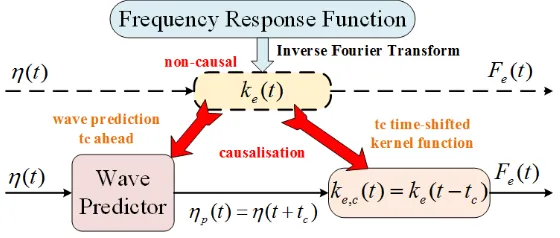
Figure 4: Schematic diagram of the W2EF modelling approach.
Since the frequency-domain response of the excitation force is available in
182
Figure 3, its time-domain kernel function ke(t) can be gained by the inverse
183
Fourier transform. However, the kernel function ke(t) characterises that the
184
W2EF process is non-causal. Therefore, a time-shift technique is applied to
185
causalise the non-causal kernel functionke(t) to its causalised formke,c(t) (see
186
Figure 4) with causalisation timetc(tc≥0). Thus, the wave elevation prediction
187
withtc in advance is required. The implementation of the W2EF modelling is
188
detailed in this Section.
189
According to the frequency-domain response in Figure 3, the excitation force
190
can be represented as:
191
whereHe(jω) is the FRF of the W2EF process. A(jω) is the frequency-domain
192
representation of the incoming wave elevationη(t).
193
Alternatively, the excitation force can be expressed in the time-domain as:
194
Fe(t) =ke(t)∗η(t) =
Z ∞
−∞
ke(t−τ)η(τ)dτ, (7) whereke(t) is the excitation force IRF related to its FRFHe(jω), given as:
195
ke(t) = 1 2π
Z ∞
−∞
He(jω)ejωtdω. (8)
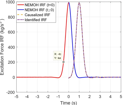
Based on the frequency-domain response in Figure 3, the kernel function
196
ke(t) is computed according to Eq. (8) and shown in Figure 5, in which the
197
red solid curve (marked NEMOH IRF (t <0)) illustrates the non-causality of
198
the W2EF process. The physical meaning of the non-causality is explained in
199
[15]. Theke(t) values for thet <0 part are almost the same as thet≥0 part.
200
Therefore, ignoring of the non-causality will in general lead to significant errors
201
in the excitation force estimation.
-5 -4 -3 -2 -1 0 1 2 3 4 5
Time (s)
-200 0 200 400 600 800 1000
Excitation Force IRF (kg/s
3 )
NEMOH IRF (t<0)
NEMOH IRF (t≥0)
Causalized IRF Identified IRF
[image:12.612.173.421.415.626.2]X: -tc Y: ke
Figure 5: Comparison of the excitation force IRFs.
To note: In [14, 15], the kernel functionke(t) is time-shifted first and then
203
treated as a curve fitting problem. However, the implementation procedure and
204
the results of the excitation force are not given in [14, 15]. In this study, both
205
the causalisation and its implementation with wave prediction are outlined in
206
this Section. The numerical and experimental results of the excitation force are
207
compared in both the time- and frequency-domains in Section 5.1.
208
As shown in Figure 4, the incident wave propagates through a non-causal
sys-209
tem characterised byke(t) and gives the excitation force approximation.
How-210
ever, this non-causal system is not implementable. Therefore, causalisation is
211
required and can be achieved with a time-shifted kernel functionke,c(t) and wave
212
predictionηp(t). The wave prediction horizon is the same as the causalisation
213
timetc.
214
According to the property of the convolution operation, this causalised
sys-215
tem with wave prediction gives the same excitation force of the non-causal
sys-216
tem [14], since:
217
Fe(t) = ke(t)∗η(t) (9)
= ke(t−tc)∗η(t+tc) (10) = ke,c(t)∗ηp(t), (11)
where
218
ke,c(t) =ke(t−tc), (12)
219
ηp(t) =η(t+tc). (13)
ke,c(t) andηp(t) are the causalised IRF of the excitation force and the predicted
220
wave elevation withtc in advance, respectively. The procedures to identify the
221
ke,c(t) and to predict theηp(t) are detailed as follows.
222
3.1.2. System Identification of Causalised Kernel Function
223
The excitation force expressed in Eq. (11) is causal if the predicted wave
224
is viewed as the system input. Hence, the convolution operation can be
ap-225
proximated by a finite order system [14, 28, 29]. In this study, realisation
theory is applied to the causalised kernel function ke,c(t) to approximate the
227
system matrices in Eqs. (14) and (15) directly with the MATLABR function
228
imp2ss [30] from the robust control toolbox. The order number of the
identi-229
fied system is quite high, as determined by ke,c(t). Hence, model reduction is
230
required and achieved using the square-root balanced model reduction method
231
with MATLABR functionbalmar [31]. 232
In this study Eq. (11) is approximated by the following state-space model:
233
˙
xe(t) = Aexe(t) +Beηp(t), (14)
Fe(t) ≈ Cexe(t), (15)
wherexe(t)∈Rn×1 is the state vector for the excitation system. A
e∈Rn×n,
234
Be ∈ Rn×1 and Ce ∈ R1×n are the system matrices. n represents the system
235
order number.
236
To identify the causalised system, the causalisation timetc and the system
237
order numbern should be selected carefully. Here a truncation error function
238
Etis defined to evaluate the causalisation time, given as:
239
Et=
R−tc
−∞|ke(t)|dt
R∞
−∞|ke(t)|dt
. (16)
For tc ∈ [0,5], the truncation error is given in Figure 6. For tc = 0.8 s, the
240
truncation error is aboutEt= 0.0104 and fortc = 2 s, the truncation error is
241
aboutEt= 0.0044. Increasing the causalisation time can decrease the
trunca-242
tion error. However, the truncation error is small enough fortc∈[0.8,2]. Thus
243
tc= 0.8 : 0.05 : 2 s is selected to determine the system order number n.
244
To further determine the causalisation time tc and the system order n, a
245
fitting-goodness function (called F G) of the causalised IRF ke,c(t) is defined
246
with a cost-function of Normalized Mean Square Error (NMSE), as:
247
F G= 1−
xref−x
xref−x¯ref
2
2
, (17)
where kXk22 and ¯X are the 2-norm and mean value of vector X, respectively.
248
The fitting-goodness tends to 1 for the best fitting and−∞for the worst fitting.
0 1 2 3 4 5
Causalisation Time t
c (s)
0 0.1 0.2 0.3 0.4 0.5
Truncation Error E
t
X: 0.8
[image:15.612.173.421.134.349.2]Y: 0.01042 X: 2Y: 0.004422
Figure 6: Truncation error of the excitation force IRF varies against the causalisation time.
The fitting-goodness of the causalised excitation IRF relies on the
causali-250
sation timetc and system order numbern. Figure 7 shows the fitting-goodness
251
function varying with the caulisation timetc = 0.8 : 0.05 : 2 s and the system
252
order numbern= 3 : 1 : 8. For a constanttc, the fitting-goodness increases as
253
the system order numbernincreases. To achieve a perfect fitting or
identifica-254
tion (such as a given fitting-goodnessF G ≥0.98), a larger causalisation time
255
requires a higher system order numbern. For instance, n= 4 givesF G≥0.98
256
fortc= 1 s andn= 5 is requred to achieveF G≥0.98 fortc = 1.2 s.
257
According to Figures 6 and 7, a system withtc= 1 s and n= 6 gives a low
258
truncation error (Et<0.01) and a good fitting of the causalised kernel function
259
ke,c(t) (F G > 0.99). Hence tc = 1 s and n = 6 are selected for this study.
260
The identified IRF is compared with the causalised and original IRFs of the
261
excitation force in Figure 5. To note,tc = 1 s is selected here to overcome the
262
non-causality of the W2EF process and to provide current information of the 263
Figure 7: Fitting-goodness with varying causalisation timetcand system order numbern.
excitation force prediction or increasing the wave prediction horizon. 265
3.1.3. Wave Prediction
266
According to Eq. (10), a short-term wave prediction is required to achieve
267
the causalisation problem in Figure 4. There are several approaches to provide
268
reasonably accurate wave predication for a short-term horizon, the notable of
269
which are: (i) the AR model approach [22], (ii) the ARMA model approach [23]
270
and (iii) the fast Fourier transform approach [32]. The real-time implementation
271
of wave prediction is discussed in [33]. In [22], wave prediction via AR model
272
shows a high accordance to the ocean waves in Irish sea. Since these techniques
273
are mature, the AR model approach developed in [22] is adopted in this study
274
to provide a short-term wave prediction.
275
For harmonic waves, wave prediction is easy to achieve. For irregular waves,
276
three campaigns of wave prediction practice using AR model are shown in
Fig-277
ure 4. The wave elevation η(t) is acquired from wave tank tests and satisfies
278
the Pierson-Moskowitz (PM) spectrum [34] with peak frequencyfp = 0.4, 0.6,
279
0.8 Hz. As suggested in [22], a low pass filter has been applied to the wave
elevation measuremtns for improving the prediction performance. The wave
281
prediction horizon is the same as the causalisation timetc and this is expressed
282
in Eq. (10). According to Figure 7,tc = 1 s is selected for the excitation force
283
approximation.
420 425 430 435 440
-20 0 20
A: PM Specturm, fp=0.4Hz, Hs=0.25m
η(t) ηp(t)
420 425 430 435 440
-10 0 10
Wave Elevation (cm)
B: PM Specturm, f
p=0.6Hz, Hs=0.11m
420 425 430 435 440
Time (s) -10
0 10
[image:17.612.178.424.209.404.2]C: PM Specturm, fp=0.8Hz, Hs=0.06m
Figure 8: Comparison of wave elevations between the experimental measurements and the
numerical predictions under irregular wave conditions.
284
For wave tank tests, the sampling frequency is 100 Hz and hence the
predic-285
tion horizon is 100 fortc= 1 s. The AR model order number is determined by
286
the goodness-of-fit index defined in [22] and hence the order number is selected
287
as 120 to keep the goodness-of-fit index larger than 70%. The order number
288
is large due to the high sampling frequency and hence it can be reduced by
289
decreasing the sampling frequency. For each campaign of wave tank tests, the
290
experimental data of 600 s are collected and divided into two parts equally. The
291
first part of data (t = 0 : 0.01 : 300 s) are used to estimate the AR model
292
parameters and the second part of data (t = 300 : 0.01 : 600 s) are used for
293
model verification. This study focuses on the verification of the W2EF method 294
and the AR model parameters are computed off-line. However, the real-time 295
on-line wave prediction can be achieved [33]. It can been seen from Figure 8
that the predicted wave elevation fits the experimental data well. However, the 297
prediction performance decreases as the peak frequency increases. For the PM 298
spectrum, higher peak frequency results in wider bandwidth and hence one po-299
tential way to improve the prediction performance is to increase the order of 300
the AR model when the peak frequency is high. In this study the AR model
301
is adopted as a wave predictor to provide future information for the identified
302
system, as shown in Figure 4.
303
3.2. PAD2EF Modelling
304
3.2.1. Outline of PAD2EF Method
[image:18.612.170.443.309.483.2]305
Figure 9: Schematic diagram of the PAD2EF modelling approach.
For an oscillating PAWEC, the excitation force can be reconstructed from its
306
sensing system. As shown in Figure 9, the total wave forceFw(t) acting on the
307
structure can be estimated from the pressure measurementp(t) on the wetted 308
surface. The hydrostatic force defined in Eq. (2) can be represented by the
309
displacement measurementz(t). The radiation force can be approximated from
310
the measurements of the velocity ˙z(t) and acceleration ¨z(t). The acceleration 311
measurement is post-processed with low pass filter since this study focuses on the 312
PAD2EF method verification rather than real-time implementation. Therefore,
the excitation force can be approximated as:
314
Fe(t) =Fw(t)−Fhs(t)−Fr(t). (18) The convolution term of the radiation force Fr(t) in Eq. (3) is approximated
315
by a finite order system [29] as follows.
316
3.2.2. Radiation Force Approximation
317
The convolution operation of the radiation force in Eq. (3) is defined as a
318
radiation subsystem, given as:
319
Fr′(t) =kr(t)∗z˙(t). (19) The kernel functionkr(t) is gained from NEMOH and shown in Figure 2. The
320
convolution approximation approach is the same as described in Section 3.1.2.
321
To determine an appropriate system order number, the fitting-goodness
func-322
tion in Eq. (17) is applied. A third order system is adopted to approximate the
323
radiation subsystem in Eq. (19) with a fitting-goodness ofF G= 0.9989, as:
324
˙
xr(t) = Arxr(t) +Brz˙(t), (20)
Fr′(t) ≈ Cr(t)xr(t), (21) where xr(t) ∈ R3×1 is the state vector for the radiation system. A
r ∈ R3×3,
325
Br ∈R3×1 and Cr ∈R1×3 are the system matrices. Therefore, the excitation
326
force can be estimated from the measurements of the pressure, acceleration and
327
displacement, given as:
328
Fe(t) =
ZZ
p(t)ds+khsz(t) +A∞z¨(t) +F ′
r(t). (22)
3.2.3. Pseudo-Velocity Measurement
329
As shown in Figure 9, the measurements of the pressure, displacement and
330
acceleration are accessible and implementable. However, the velocity
measure-331
ment is difficult and expensive to obtain. A “pseudo-velocity” can be
esti-332
mated/observed from the displacement/acceleration measurements. In [19], the
333
velocity is obtained from the first order derivative of an accurate displacement
measurement with a high sampling frequency. The drawbacks of this approach
335
are: (i) the velocity estimation is infected by the measurement noise and (ii) the
336
velocity estimation is always one sample period behind the real velocity (high
337
sampling frequency is required).
338
In this work, a carefully designed Band-Pass Filter (BPF) is applied to obtain
339
the velocity estimate from the displacement measurement. Compared with the
340
differentiation approach, a velocity estimate with less phase lag can be gained
341
via the BPF. The second order BPF is given as:
342
BP F(s) = Abpf ωc
Qbpfs
s2+ ωc
Qbpfs+ω
2
c
, (23)
where Abpf is the amplitude gain at the central frequency ωc and Qbpf is the
343
quality factor. The drawbacks of this BPF method are: (i) the velocity
es-344
timation is influenced by measurement noise and (ii) the BPF is difficult to
345
implement with analogue filter. However, the BPF is applicable in a software
346
digital filtering way. Additionally, the velocity can be observed via an
appro-347
priately designed observer and this part of work is detailed in Section 3.3.3.
348
A variety of wave tank tests are conducted under irregular wave conditions
349
and the comparison of the pseudo-velocity measurements between the
differen-350
tial, BPF and observation methods is given in Figure 10. The pseudo-velocity
351
measurements via these three methods shows a high accordance to each other
352
due to: (i) thesamping frequency (100 Hz) is very large compared with the wave
353
frequency (1.2 Hz) and (ii) the displacement measurement is accurate enough.
354
The differential method requires high sampling frequency and accurate displace-355
ment measurement. The BPF approach calls for largeAbpf andQbpf and this
356
may result in instability of the closed-loop control system. The third method of 357
observing the velocity is preferred since the observer design is easy, robust and 358
340 342 344 346 348 350 352 354 356 358 360 -0.5
0 0.5
A: PM Spectrum, fp=0.4Hz, Hs=0.25m
Differential BPF Observed
340 342 344 346 348 350 352 354 356 358 360
-0.4 -0.2 0 0.2
Pseudo-measured Velocity (m/s)
B: PM Spectrum, fp=0.6Hz, Hs=0.11m
340 342 344 346 348 350 352 354 356 358 360
Time (s)
-0.2 0 0.2
[image:21.612.182.422.167.358.2]C: PM Spectrum, fp=0.8Hz, Hs=0.06m
Figure 10: Comparison of pseudo-measured velocity under irregular wave conditions.
[image:21.612.171.442.466.613.2]3.3. UIOEF Modelling
360
3.3.1. Outline of UIOEF Method
361
As the convolution term of the radiation force in Eq. (19) is approximated
362
by a state-space model in Eqs. (20) and (21), the PAWEC motion under the
363
wave excitation can be represented in a state-space form. Therefore, an
appro-364
priately designed UIO can be applied to estimate the unknown excitation force.
365
As shown in Figure 11, a generic UIO is applied to estimate the excitation
366
force and buoy velocity from the displacement measurement. The estimated
367
excitation force is used to generate the velocity reference, whilst the estimated
368
velocity is viewed as the velocity measurement to provide feedback for the
con-369
troller. However, this study focuses on the UIO estimator design rather than on
370
the controller structure and design. This method is referred to as the UIOEF
371
modelling method.
372
3.3.2. Force-To-Motion Modelling
373
According to Eq. (1), the PAWEC starts to oscillate under the stimulation
374
of the excitation and PTO forces. The PAWEC motion with excitation force
375
input is defined as the Force-To-Motion (F2M) model. Considering the radiation
376
approximation in Eqs. (20) and (21), the F2M model is re-written as:
377
xf2m = [z z˙ xr]T, (24)
˙
xf2m(t) = Af2mxf2m(t) +Bf2mFe(t) +Bf2mFpto(t), (25)
yf2m(t) = Cf2mxf2m(t), (26)
with
378
Af2m =
0 1 0
−khs
Mt 0 −
Cr
Mt
0 Br Ar
, (27)
Bf2m =
h
0 − 1
Mt 0
iT
, (28)
Cf2m =
h
where Mt = M +A∞ represents the total mass. xf2m(t)∈ R5×1 is the F2M 379
state vector. Af2m ∈ R5×5, Bf2m ∈ R5×1 and Cf2m ∈ R1×5 are the system
380
matrices.
381
3.3.3. Unknown Input Observer Design
382
To estimate the unknown excitation forceFe(t), it is viewed as an augmented
383
state to the system in Eqs. (25) and (26). Thus the augmented system can be
384
written as:
385
xg = [xf2m Fe]T, (30)
˙
xg(t) = Agxg(t) +BgFpto(t) +DgF˙e, (31)
yg(t) = Cgxg(t), (32)
with
386
Ag =
Af2m Bf2m
0 0
, (33)
Bg =
h
Bf2m 0
iT
, (34)
Dg =
h
0 1
iT
, (35)
Cg =
h
Cf2m 0
i
, (36)
where xg(t) ∈R6×1 is the state vector of the augmented system. A
g ∈R6×6,
387
Bg∈R6×1,Dg∈R6×1and Cg∈R1×6are the system matrices.
388
The following UIO is adapted from [35, 36] to estimate the augmented system
389
state, given as:
390
˙
xo(t) = P xo(t) +GFpto(t) +Lyf2m(t), (37)
ˆ
xg(t) = xo(t) +Qyf2m(t), (38)
where xo(t)∈R6×1 is the UIO state vector. P ∈
R6×6, G∈
R6×1, L∈
R6×1
391
and Q∈R6×1 are the UIO system matrices. ˆxg(t) represents the estimate of
392
xg(t).
393
Since the excitation force is unknown, its derivative ˙Fe(t) in Eq. (31) is
inac-394
cessible and hence viewed as a disturbance. To achieve an accurate estimation
Figure 12: Sketch of the wave tank and the device installation.
of the excitation force, theH∞robust optimisation approach is applied to
com-396
pute the observer matricesP,G,LandQto reject the influence of ˙Fe(t), using
397
the MATLABR LMI toolbox. The computation of the observer gain matrixL 398
follows the method described in [36] and is thus omitted here.
399
4. Wave Tank Tests 400
4.1. Experiment Settings
401
To verify the excitation force estimations via the W2EF, PAD2EF and
402
UIOEF approaches, a series of wave tank tests have been conducted. As shown
403
in Figure 12, the wave tank is 13 m in length, 6 m in width and 2 m in height
404
(with water depth 0.9 m). Up to 8 pistons can be selected to generate
regu-405
lar/irregular waves.
406
The PAWEC is scaled down according to the Froude Number defined in
407
[37]. For this application the geometric ratio is selected as 1/50. Therefore, the
408
time ratio is 1/7.0711. For ocean waves of sea state 7 defined by the Beaufort
409
scale [38], its characteristics can be represented by a PM spectrum with peak
410
frequencyfp = 0.095 Hz and significant wave height Hs = 4.3 m. The scaled
411
down PM spectrum (according to the Froude Number) is featured by the peak
412
frequency fp = 0.0952×7.0711 = 0.67 Hz and significant wave height Hs =
4.3/50 = 0.086 m. Therefore, the wave conditions in the wave tank tests are
414
configured with wave frequencies as f = 0.4 : 0.1 : 1.2 Hz and wave height
415
H = 0.08 m for regular waves. For irregular waves, the peak frequencies of the
416
PM spectra are selected asfp= 0.4,0.6,0.8 Hz.
417
The 1/50 scale cylindrical heaving PAWEC has been simulated, designed and
418
constructed for wave tank tests, model verification and control system design, as
419
shown in Figure 12. Five Wave Gauges (WGs) are mounted to measure the water
420
elevation in real-time, with WG1&2 in the up-stream, WG3 in line with the buoy
421
and WG4&5 in the down-stream. For this study, only the WG3 measurement 422
is used. WG1&2 and WG4&5 are useful to estimate the reflection of the wave 423
tank end wall and to verify the generated irregular wave satisfies the pre-set PM 424
spectrum. Six Pressure Sensors (PSs) are applied in the wave tank tests with
425
PS1-5 installed at the bottom of the PAWEC to measure the dynamic pressure
426
acting on the hull and PS6 fixed in line with WG1 for synchronisation1. A Linear 427
Variable Displacement Transducer (LVDT) and a 3-axis Accelerometer (Acc) are
428
rigidly connected with the oscillating body to provide motion measurements.
429
All these sensing signals are collected by a data acquisition system connected
430
with LABVIEWTM panel. The sampling frequency is 100 Hz. The pressure, 431
displacement and acceleration measurements are post-processed with low pass 432
filters to verify the modelling and estimation concepts. 433
For the excitation tests, the PAWEC is fixed semi-submerged and under
434
the excitation of incident waves to verify the W2EF modelling approach. For
435
the wave-excited-motion tests, the buoy is forced to oscillate from zero-initial
436
condition under the excitation of incoming waves. Since this study has a specific
437
1The installation depth of PS6 is 0.4 m. There are two sensing systems applied: one
integrated with the wave maker and the other designed for the PAWEC. It is a good idea to
isolate the electrical connects of these two sensing systems in case there are some penitential
conflicts. The PAWEC sensing system triggers the wave maker sensing system. However,
there is still a small time shift between these two sensing systems due to different design of
the hardware and software. Thus PS6 and WG1 are installed to measure the same signal to
focus on the estimations of the excitation force, the control or PTO force is set as
438
Fpto= 0 N for the excitation tests orthe wave-excited-motiontests. For control
439
practice,Fptois known and hence it is applicable to obtain the excitation force
440
by subtracting Fpto from the estimate of PAD2EF or UIOEF approaches. If
441
Fpto is not known, only the W2EF method is applicable.
442
4.2. Excitation Tests
443
For the excitation tests, the PAWEC is fixed to the wave tank gantry at
444
its equilibrium point and excited by the incident wave. The pressure sensors
445
installed at the bottom of the buoy provide the measurement of the dynamic
446
pressure acting on the hull. Thus, the wave excitation force in heave can be
447
represented as:
448
Fe(t) =
ZZ
p(t)ds≈πr2p¯(t), (39)
where ¯p(t) represents the average value of the five pressure sensors (PS1-5).
449
Note that Eq. (39) only gives an simple approximation of the the excitation
450
force. When the buoy diameter is relative small to the wavelength (such as
451
tenth of the wavelength), the accuracy of Eq. (39) is acceptable. If the buoy
452
dimension is almost the same scale of the wavelength, more pressure sensors are
453
required to achieve accurate excitation force measurement.
454
Meanwhile, five WGs are installed to measure the wave elevation, amongst
455
which, WG3, is in line with the buoy. The measurement of WG3 represents
456
the incident wave at the center of the PAWEC and is adopted to provide wave
457
prediction in a short-term horizon tc. A wide variety of excitation tests
un-458
der regular and irregular wave conditions are conducted to verify the W2EF
459
modelling approach. The numerical and experimental results are compared and
460
discussed in Section 5.1.
461
4.3. Wave-excited-motion Tests
462
For the wave-excited-motion tests, the PAWEC is forced to oscillate from
463
its zero-initial condition under the excitation of the incident waves. In this
situation, the measurements from pressure sensors represent the total wave force
465
rather than the excitation force, given as:
466
Fw(t) =
ZZ
p(t)ds≈πr2p¯(t). (40)
Also, Eq. (40) is valid only when the buoy dimension is relatively small
com-467
pared with the wavelength.
468
Meanwhile, the buoy acceleration and displacement are measured by the
469
accelerometer and LVDT, respectively. Therefore, the excitation force can be
470
estimated via the PAD2EF approach in Eq. (22). Also, the wave elevation
471
measurements are accessible. Thus the W2EF method can be applied on WG3
472
measurement to approximate the excitation force according to Eqs. (14) and
473
(15). Since the displacement measurement is accessible, the UIOEF approach
474
in Eqs. (37) and (38) can be applied to estimate the excitation force as well.
475
The numerical and experimental comparison of the excitation force between the
476
W2EF, PAD2EF and UIOEF approaches is discussed in Section 5.2.
477
5. Results and Discussion 478
5.1. Results of Excitation Tests
479
Since the PAWEC is fixed during the excitation tests. The motion
measure-480
ments are not applicable. Therefore, only the W2EF approach can be applied to
481
estimate the excitation force. To verify the proposed W2EF modelling approach,
482
excitation tests are conducted under regular and irregular wave conditions and
483
the experimental data are compared with the numerical simulations of Eqs. (14)
484
and (15).
485
5.1.1. Regular Wave Conditions
486
Nine excitation tests are conducted under regular waves with wave height
487
H = 0.08 m and frequencies f = 0.4 : 0.1 : 1.2 Hz. For harmonic waves,
488
precise wave prediction withtc = 1 s in advance is easy to achieve. Recall that
489
the prediction horizon is the same as the causalisation time illustrated in Eq.
85 86 87 88 89 90
Time (s)
-20 -15 -10 -5 0 5 10 15 20
Excitation Force (N)
-10 -5 0 5 10
Wave Elevation (cm)
[image:28.612.184.441.136.327.2]Measured Fe Identified Fe Wave Elevation
Figure 13: Comparison of the excitation forces between the measurement and the estimate
via W2EF method.
(10) and Figure 7. Therefore, the W2EF modelling approach always provides
491
accurate approximation of the excitation force under regular waves. For the
492
harmonic wave with frequencyf = 0.7 Hz, the excitation force measurement in
493
Eq. (39) and the estimation in Eqs. (14) and (15) are compared in Figure 13.
494
The estimation via W2EF method shows a high accordance to the experimental
495
data, which indicates the validity of the W2EF method for excitation tests under
496
regular wave conditions.
497
To check the fidelity further, the excitation force FRF is compared with the
498
W2EF result as well as the NEMOH computation. The amplitude and phase
499
responses are shown in Figure 14 and Figure 15, respectively. The amplitude
500
response of the W2EF method fits the NEMOH and excitation tests data to a
501
high degree. This is why the analytical representations of the excitation force
502
in Eqs. (4) and (5) are widely adopted to investigate WEC dynamics. Note
503
that the excitation force amplitude response is normalised with respect to the
504
hydrostatic stiffnesskhs.
505
Figure 15 compares the experimental and numerical phase responses from
0 2 4 6 8 10 12
ω (rad/s)
0 0.2 0.4 0.6 0.8 1
Normalised Amplitude Response of F
e NEMOH Results
[image:29.612.176.421.135.328.2]Identified System Experimental Data
Figure 14: Amplitude response comparison of the excitation force amongst the excitation
tests, NEMOH computations and W2EF simulations.
the incident wave η(t) to the excitation forceFe(t) in Eq. (9). A good
accor-507
dance of the phase response means that the W2EF modelling approach with
508
kernel function causlisation and wave prediction in Eq. (11) gives almost the
509
same system description of the non-causal system in Eq. (9). Also, Figure 510
15 illustrates that the analytical representations of the excitation force in Eqs. 511
(4) is improper for PAWEC modelling and control design, especially when the 512
frequency is relatively high. Note that, the excitation force phase response is 513
normalised with respect toπ.
514
5.1.2. Irregular Wave Conditions
515
Irregular waves characterised by the PM spectrum are adopted in the
exci-516
tation tests and the results are shown in Figure 16. Generally speaking, the
517
estimated excitation force via the W2EF method shows a good accordance
518
to the experimental data for most of the time. The estimation only varies
519
a bit from the measurement when the wave elevation is occasionally small.
520
0 2 4 6 8 10 12
(rad/s)
-0.1 0 0.1 0.2 0.3 0.4 0.5 0.6
Normalised Phase Response of F
e
[image:30.612.173.422.135.351.2]NEMOH Results Identified System Experimental Data
Figure 15: Phase response comparison of the excitation force amongst the excitation tests,
NEMOH computations and W2EF simulations.
t = 436−440 s in Figure 16, case A. However, this part is not important
522
from the viewpoint of power maximisation. For the irregular wave condition
523
of fp = 0.8 Hz, Hs = 0.06 m, the excitation force estimate is not as accurate
524
as that for the other two wave conditions. The potential reason may be the
525
inaccuracy in Eq. (39) since the point absorber assumption are not fully
sat-526
isfied. Additionally, the wave elevation predictions corresponding to Figure 16
527
are given in Figure 8.
528
5.2. Results ofWave-excited-motionTests
529
For thewave-excited-motion tests, the PAWEC oscillates under the
excita-530
tion of incident waves. Therefore, the pressure, displacement and acceleration
531
measurements, together with the wave elevation, are available. Thus the W2EF,
532
PAD2EF and UIOEF approaches are adopted to approximate the excitation
533
force acting on the PAWEC hull. In thewave-excited-motiontests, the
excita-534
tion force is immeasurable since the pressure sensors give the total wave force
420 422 424 426 428 430 432 434 436 438 440 -50
0 50
A: PM Specturm, fp=0.4Hz, Hs=0.25m
Measured Fe Identified Fe
420 422 424 426 428 430 432 434 436 438 440
-40 -20 0 20 40
Excitation Force (N)
B: PM Specturm, f
p=0.6Hz, Hs=0.11m
420 422 424 426 428 430 432 434 436 438 440
Time (s)
-20 0 20
[image:31.612.185.422.132.324.2]C: PM Specturm, fp=0.8Hz, Hs=0.06m
Figure 16: Comparison of the excitation force between the excitation tests and the W2EF
modelling under irregular wave conditions.
Fw(t) in Eqs. (18) and (40).
536
Three campaigns of wave-excited-motion tests are conducted under
irreg-537
ular wave conditions and the excitation force comparison among the W2EF,
538
PAD2EF and UIOEF approximation approaches is given in Figure 17. Since
539
the excitation force cannot be measured directly, it is very hard to say which
540
method is better. Via the comparison in Figure 17, it is found that: (i) All these
541
three methods give good estimation of the excitation force when the wave (or
542
excitation force) is large for the wave conditions offp = 0.4 Hz, Hs= 0.25 m
543
andfp= 0.6 Hz, Hs= 0.11 m. (ii) When the wave is small or changes rapidly,
544
the estimations given by the PAD2EF and UIOEF approaches are more
vari-545
able, compared with the W2EF estimation. Compared to the excitation force, 546
the radiation approximation error and non-linear friction/viscous forces [39] are 547
relatively large. (iii) Generally speaking, the magnitude of the excitation force
548
approximation given by the W2EF method is smaller than the ones provided
549
by the PAD2EF and UIOEF approaches. One potential reason is that the wave
550
gauge measurement is attenuated by the interference between the incident and
340 342 344 346 348 350 352 354 356 358 360 Time (s)
-50 0 50
Excitation Force Estimation (N)
W2EF PAD2EF UIOEF
(a) PM spectrum,fp= 0.4 Hz, Hs= 0.25 m.
340 342 344 346 348 350 352 354 356 358 360 Time (s)
-30 -20 -10 0 10 20 30
Excitation Force Estimation (N)
W2EF PAD2EF UIOEF
(b) PM spectrum,fp= 0.6 Hz, Hs= 0.11 m.
340 342 344 346 348 350 352 354 356 358 360 Time (s)
-15 -10 -5 0 5 10 15
Excitation Force Estimation (N)
W2EF PAD2EF UIOEF
[image:32.612.168.434.179.607.2](c) PM spectrum,fp= 0.8 Hz, Hs= 0.06 m.
radiated waves [16]. (iv) For the wave condition offp= 0.8 Hz, Hs= 0.06 m, the
552
W2EF method gives slightly better estimation than the PAD2EF and UIOEF
553
approaches. One potential reason is that the wave excitation force is small
554
under this wave condition and hence the mechanical friction force is relative
555
large. The PAD2EF and UIOEF methods in this work cannot decouple the
me-556
chanical friction force from there excitation force estimations. For the specified 557
1/50 PAWEC, the friction can be characterised experimentally [39]. Whilst the
558
W2EF method estimates the wave excitation force from wave measurements
559
and hence the estimates are not affected by mechanical friction force.
560
A comparison of these methods are made as follows:
561
• The W2EF modelling approach requires the wave elevation measurement
562
only. The W2EF approach shows advantages in easy implementation and
563
good tolerance to the mechanical friction and fluid viscous forces.
How-564
ever, the W2EF approach is subjected to linear wave theory and small
565
radiated wave. Additionally, accurate wave prediction is compulsory to
566
overcome the non-causality of the W2EF process.
567
• The PAD2EF modelling method requires the measurements of pressure,
568
acceleration and displacement. Hence it is complex to implement. The
569
PAD2EF estimation is affected by the modelling error of the radiation 570
force approximation and fluid viscous force but not the mechanical
fric-571
tion force and radiated wave. Another advantage is that the PAD2EF
572
estimation is applicable when the incident waves are non-linear or when
573
the W2EF process is non-linear.
574
• The UIOEF modelling approach only requires the displacement
measure-575
ment. Thus it is easy to implement. Also, the UIOEF estimation does not
576
suffer from the radiated wave but is influenced bymodelling error of the 577
radiation force approximation, the mechanical friction and fluid viscous
578
forces. Also, the UIOEF method can be applied under the excitation of
579
non-linear incident waves.
For the control structure in Figure 11, the estimation error of the excitation
581
force will affect the power capture performance. This part of work has been
582
investigated in [40] and it shows that the influence of the estimation error on
583
the power capture can be attenuated at certain band of frequencies via robust
584
control design.
585
6. Conclusion 586
This study focuses on the modelling of the excitation force and the model
587
verification via wave tank tests. The excitation force can be approximated
588
with reasonable accuracy from the measurements of wave elevation, pressure,
589
acceleration and displacement. Therefore, the W2EF, PAD2EF and UIOEF
590
modelling approaches are proposed, simulated and tested in a wave tank. The
591
experimental data show a high accordance to the estimations of the W2EF,
592
PAD2EF and UIOEF methods. However, the application scenarios of these
593
approaches vary, as shown below:
594
• The W2EF method in Eqs. (14) and (15) gives reasonably accurate
es-595
timation of the excitation force based on the conditions: (i) the incident
596
wave is linear; (ii) the radiated wave due to the PAWEC motion is small
597
compared to the incident wave; (iii) wave elevation measurement and its
598
precise prediction are accessible.
599
• The PAD2EF approach in Eq. (22) can provide good estimation of the
600
excitation force if the following conditions are satisfied: (i) the
measure-601
ments of pressure, acceleration and displacement are available and (ii) the
602
fluid viscous force is negligible.
603
• The UIOEF strategy in Eqs. (37) and (38) only depends on the
displace-604
ment measurement and can provide precise estimation of the excitation
605
force and the velocity. But the mechanical friction and fluid viscous forces
606
cannot be decoupled from the excitation force estimation.
A wide variety of excitation tests and wave-excited-motion tests are
con-608
ducted in a wave tank to verify the proposed excitation force approximation
ap-609
proaches. The experimental data collected from the excitation tests fit with the
610
W2EF model numerical results to a high degree in both time- and
frequency-611
domains under regular and irregular wave conditions. For the wave-excited-612
motion tests, all the W2EF, PAD2EF and UIOEF modelling approaches are
613
applied to estimate the excitation force and their estimations show high
accor-614
dance to each other when buoy dimension is relatively small to the incident
615
wavelength.
616
Therefore, these proposed excitation force approximation approaches can be
617
useful for the performance assessment and real-time power maximisation control
618
of WEC systems. Ongoing work focuses on the excitation force prediction and
619
its implementation for the MPC on WEC systems.
620
Acknowledgment 621
Bingyong Guo, Siya Jin and Jianglin Lan thank the China Scholarship
Coun-622
cil and the University of Hull for joint scholarships. Thanks are expressed to
623
Professor Dan Parsons, Dr Stuart McLelland and Mr Brendan Murphy of the
624
School of Environmental Sciences for their help and supervision in using the
625
Hull University wave tank.
626
Appendix 627
The buoy dimensions are: radius r = 0.15 m, height b = 0.56 m, draft
628
d = 0.28 m, mass M = 19.79 kg, water density ρ = 1000 kg/m3, gravity
629
constant g = 9.81 N/kg, hydrostatic stiffness khs = 693.43 N/m and added
630
mass at infinite frequencyA∞= 6.58 kg.
The system matrices of the W2EF system in Eqs. (14) and (15) are:
632
Ae =
−0.234 1.818 0.530 −0.554 −0.314 −0.054
−1.818 −0.900 −3.043 1.082 0.861 0.130 0.530 3.044 −1.798 4.233 1.553 0.306 0.554 1.082 −4.233 −2.688 −5.096 −0.480
−0.314 −0.861 1.553 5.096 −3.590 −3.064 0.054 0.130 −0.306 −0.480 3.064 −0.157
, (41)
Be =
h
164.34 251.36 −236.52 −175.67 114.01 −18.71
iT
,(42)
Ce =
h
1.6434 −2.5136 −2.3652 1.7567 1.1401 0.1871.
i
. (43) The system matrices for the identified radiation subsystem in Eqs. (20) and
633
(21) are:
634
Ar =
−3.1848 −4.3372 −3.1009 4.3372 −0.0875 −0.3882 3.1009 −0.3882 −2.8499
, (44)
Br =
h
−40.6964 5.9737 16.2722
iT
, (45)
Cr =
h
−0.4070 −0.0597 −0.1627 i. (46) The parameters of the BPF in Eq. (23) are: ωc = 8π rad/s, Abpf = 2433
635
andQbpf = 100.
636
The system matrices of the UIO in Eqs. (37) and (37) are:
637 P =
−0.57 9.01 0 0 0 0
−27.09 −39.1 0.02 0.02 0.01 0.04
−3.24 −0.13 −3.18 −4.34 −3.1 0
−0.95 0.43 4.34 −0.09 −0.39 0 0.2 −1.62 3.10 −0.39 −2.85 0
−32856 −242450 0 0 0 0
, (47)
G = h 0 0.0379 0 0 0 0
iT
, (48)
L = h 357.52 7881.9 73.80 −158.04 −244.25 −9183200 i T
Q = h −8.01 39.1 −40.57 5.55 17.89 242450 i T
. (50)
To note: The feedback gains of the UIO are large and sensitive to measurement
638
noise. It is due to the system property since the magnitude of the displacement
639
z(t) is 10−2 and the magnitude of the excitation force Fe(t) is 10. Thus this
640
is a numerical stiffness or conditioning problem with varying ratio 103. In 641
real operation, a low pass filter is applied to the displacement measurement to
642
attenuate the noise.
643
References 644
[1] M. McCormick, Ocean wave energy conversion, Wiley-Interscience, New
645
York, 1981.
646
[2] F. d. O. Antonio, Wave energy utilization: A review of the technologies,
647
Renew. Sustainable Energy Rev. 14 (3) (2010) 899–918.
648
[3] B. Drew, A. Plummer, M. N. Sahinkaya, A review of wave energy converter
649
technology, P. I. Mech. A-J Pow. 223 (8) (2009) 887–902.
650
[4] A. Cl´ement, P. McCullen, A. Falc˜ao, A. Fiorentino, F. Gardner, K.
Ham-651
marlund, G. Lemonis, T. Lewis, K. Nielsen, S. Petroncini, et al., Wave
652
energy in Europe: current status and perspectives, Renew. Sust. Energ.
653
Rev. 6 (5) (2002) 405–431.
654
[5] J. V. Ringwood, G. Bacelli, F. Fusco, Energy-maximizing control of
wave-655
energy converters: The development of control system technology to
opti-656
mize their operation, IEEE Control Systems 34 (5) (2014) 30–55.
657
[6] S. Salter, Power conversion systems for ducks, in: Proc. of the International
658
Conference on Future Energy Concepts, Vol. 1, 1979, pp. 100–108.
659
[7] K. Budal, J. Falnes, Optimum operation of improved wave-power converter,
660
Mar. Sci. Commun. 3 (2) (1977) 133–150.
[8] A. Babarit, M. Guglielmi, A. H. Cl´ement, Declutching control of a wave
662
energy converter, Ocean Eng. 36 (12) (2009) 1015–1024.
663
[9] G. Li, M. R. Belmont, Model predictive control of sea wave energy
664
converters–part i: A convex approach for the case of a single device, Renew.
665
Energy 69 (2014) 453–463.
666
[10] G. Li, M. R. Belmont, Model predictive control of sea wave energy
667
converters–part ii: The case of an array of devices, Renew. Energy 68
668
(2014) 540–549.
669
[11] J. N. Newman, The exciting forces on fixed bodies in waves, Journal of
670
Ship Research 4 (1962) 10–17.
671
[12] M. Greenhow, S. White, Optimal heave motion of some axisymmetric wave
672
energy devices in sinusoidal waves, Appl. Ocean Res. 19 (3-4) (1997) 141–
673
159.
674
[13] A. Babarit, J. Hals, M. Muliawan, A. Kurniawan, T. Moan, J. Krokstad,
675
Numerical benchmarking study of a selection of wave energy converters,
676
Renew. Energy 41 (2012) 44–63.
677
[14] Z. Yu, J. Falnes, State-space modelling of a vertical cylinder in heave, Appl.
678
Ocean Res. 17 (5) (1995) 265–275.
679
[15] J. Falnes, On non-causal impulse response functions related to propagating
680
water waves, Appl. Ocean Res. 17 (6) (1995) 379–389.
681
[16] G. Bacelli, R. G. Coe, D. Patterson, D. Wilson, System identification of a
682
heaving point absorber: Design of experiment and device modeling,
Ener-683
gies 10 (4) (2017) 472.
684
[17] S. Giorgi, J. Davidson, J. Ringwood, Identification of nonlinear excitation
685
force kernels using numerical wave tank experiments, in: Proc. EWTEC,
686
Nantes, France, 2015, pp. 09C1–1–1–09C1–1–10.
[18] B. A. Ling, Real-time estimation and prediction of wave excitation forces for
688
wave energy control applications, Master’s thesis, Mechanical Engineering,
689
Oregon State University (2015).
690
[19] O. Abdelkhalik, S. Zou, G. Bacelli, R. D. Robinett, D. G. Wilson, R. G.
691
Coe, Estimation of excitation force on wave energy converters using
pres-692
sure measurements for feedback control, in: Proc. OCEANS MTS/IEEE
693
Monterey, IEEE, 2016, pp. 1–6.
694
[20] G. Bacelli, R. G. Coe, State estimation for wave energy converters, Tech.
695
rep., Sandia National Laboratories (SNL-NM), Albuquerque, NM (United
696
States) (2017).
697
[21] M. Abdelrahman, R. Patton, B. Guo, J. Lan, Estimation of wave excitation
698
force for wave energy converters, in: Proc. SysTol, IEEE, 2016, pp. 654–
699
659.
700
[22] F. Fusco, J. V. Ringwood, Short-term wave forecasting for real-time control
701
of wave energy converters, IEEE Trans. Sustain. Energy 1 (2) (2010) 99–
702
106.
703
[23] M. Ge, E. C. Kerrigan, Short-term ocean wave forecasting using an
au-704
toregressive moving average model, in: Proc. UKACC, IEEE, 2016, pp.
705
1–6.
706
[24] J. Falnes, Ocean waves and oscillating systems: linear interactions including
707
wave-energy extraction, Cambridge University Press, 2002.
708
[25] W. Cummins, The impulse response function and ship motions, Tech. rep.,
709
DTIC Document (1962).
710
[26] G. Giorgi, J. V. Ringwood, Implementation of latching control in a
nu-711
merical wave tank with regular waves, Journal of Ocean Engineering and
712
Marine Energy 2 (2) (2016) 211–226.