Forced Gravity Waves and the Tropospheric Response to Convection

Convection

.

White Rose Research Online URL for this paper:

http://eprints.whiterose.ac.uk/128507/

Version: Accepted Version

Article:

Halliday, OJ orcid.org/0000-0002-8863-9081, Griffiths, SD

orcid.org/0000-0002-4654-2636, Parker, DJ orcid.org/0000-0003-2335-8198 et al. (2 more

authors) (2018) Forced Gravity Waves and the Tropospheric Response to Convection.

Quarterly Journal of the Royal Meteorological Society, 144 (712). Part A. pp. 917-933.

ISSN 0035-9009

https://doi.org/10.1002/qj.3278

eprints@whiterose.ac.uk https://eprints.whiterose.ac.uk/ Reuse

Items deposited in White Rose Research Online are protected by copyright, with all rights reserved unless indicated otherwise. They may be downloaded and/or printed for private study, or other acts as permitted by national copyright laws. The publisher or other rights holders may allow further reproduction and re-use of the full text version. This is indicated by the licence information on the White Rose Research Online record for the item.

Takedown

If you consider content in White Rose Research Online to be in breach of UK law, please notify us by

Forced Gravity Waves and the Tropospheric Response to

Convection

Oliver J. Halliday

, Stephen D. Griffiths

, Douglas J. Parker

, Alison Stirling

and Simon Vosper

a_{Institute for Climate and Atmospheric Science, School of Earth and Environment, University of Leeds, UK}

b_{Department of Applied Mathematics, University of Leeds, UK}

c_{Met Office, UK}

∗_{Correspondence to: O. J. Halliday, Institute for Climate and Atmospheric Science, University of Leeds, Leeds, LS2 9JT. E-mail:}

mm10ojh@leeds.ac.uk

We present theoretical work directed toward improving our understanding of the

mesoscale influence of deep convection on its tropospheric environment through forced

gravity waves. From the linear, hydrostatic, non-rotating, incompressible equations,

we find a two-dimensional analytical solution to prescribed heating in a stratified

atmosphere, which is upwardly radiating from the troposphere when the domain lid is

sufficiently high. We interrogate the spatial and temporal sensitivity of both the vertical

velocity and potential temperature to different heating functions, considering both the

near-field and remote responses to steady and pulsed heating. We find that the mesoscale

tropospheric response to convection is significantly dependent on the upward radiation

characteristics of the gravity waves, which are in turn dependent upon the temporal and

spatial structure of the source, and the assumed stratification. We find a 50% reduction

in tropospherically averaged vertical velocity when moving from a trapped (i.e. low lid)

to upwardly-radiating (i.e. high lid) solution, but even with maximal upward radiation,

we still observe significant tropospheric vertical velocities in the far-field 4 hours after

heating ends. We quantify the errors associated with coarsening a 10 km wide heating to

a 100 km grid (in the way a General Circulation Model (GCM) would), observing a 20%

reduction in vertical velocity. The implications of these results for the parameterisation

of convection in low-resolution numerical models are quantified and it is shown that

the smoothing of heating over a grid-box leads to significant in grid-box tendencies,

due to the erroneous rate of transfer of compensating subsidence to neighbouring

regions. Further, we explore a simple time-dependent heating parameterisation that

minimises error in a parent GCM grid box, albeit at the expense of increased error

in the neighbourhood.

c

1. Introduction

Tropical deep convection is observed to be organised on the

synoptic and mesoscale (Wheeler and Kiladis 1999; Tulich et al.

2007), and it is argued that gravity waves provide a mechanism

for the aggregation of cumulonimbus storms (Tulich et al. 2011)

as they communicate the necessary atmospheric adjustment to

the neighbouring troposphere through subsidence or lifting. The

“gregarious” nature of mesoscale tropical convection cells is

thought to be driven (at least in part) by a low-level rising mode

in the vicinity of a convecting storm, which increases the depth

of moisture at low-levels, making conditions more favourable

for new convective events (Mapes 1993; Fovell et al. 1992).

Momentum and temperature changes, communicated through the

propagation of convectively generated gravity waves may also

condition the remote troposphere to convection triggering or

suppression (Bretherton and Smolarkiewicz 1989; Pandya et al.

2000; Shige and Satomura 2000).

In current General Circulation Models (GCMs) deep

convec-tion is represented as a sub-grid process, and so a theoretical

understanding of the way in which convective heating gives rise

to tropospheric adjustment is essential. A sub-grid convection

scheme adjusts the temperature, moisture and cloud fields within

a grid column, leaving the resolved dynamics to propagate this

adjustment more remotely, and thus influencing the convective

available potential energy (CAPE) of the wider environment

(Stensrud 2009). Therefore, the dynamical response to convection

is highly dependent upon the model convection scheme, which

itself is sensitive to the closures and assumptions placed upon the

parameterisations. There are a number of types of deep

convec-tive parametrisation scheme in operational use (Stensrud 2009).

Typically, a convection scheme attempts to represent an ensemble

of clouds within a given gridbox through a bulk formulation. For

instance the Gregory and Rowntree mass-flux scheme used in

the MetUM (Gregory and Rowntree 1990; Walters et al. 2017)

models the effects of entrainment and detrainment on the

ensem-ble convective-cloud mass flux through analogy with a single

plume in the gridbox. The resulting tendencies are applied at the

grid scale, and it is assumed that all compensating subsidence

occurs within that gridbox (in reality it has long been known that

gravity waves propagate laterally to move the zones of subsidence

away from the location of the forcing, e.g. Yanai et al. 1973).

While gravity-wave modes are themselves represented only by the

resolved grid, representation of thedragcaused by gravity-wave

breaking, and initiated by sub-grid orography (and sometimes

precipitating convection) is parametrised separately (e.g. Walters

et al. 2017, Bushell et al. 2015). Some sub-grid statistics of

the cloud field are diagnosed in the model (via the Prognostic

Cloud Scheme), but these are principally used to interact with

the radiation scheme and do not feed back on to the dynamic,

thermodynamic and cloud fields at present.

In summary, while current convection schemes hold some

information about the subgrid cloud field, they do not use any

subgrid cloud information in the excitation of gravity waves:

waves are only forced by the grid-resolved tendencies imposed

by the convection scheme. This leads to a possible mis-match

between the true field of gravity waves excited by subgrid

convection on the kilometre scale and the gravity waves forced

on the grid scale by the convection scheme. It is still an open

question whether such effects need to be handled explicitly in

convection schemes, or whether the model grid will handle them

satisfactorily.

Gravity waves modify the troposphere through vertical motion.

If the vertical motion at low levels is strong, of the order of metres

per second as may occur in a trapped gravity wave or bore, then

this may directly trigger deep convection (Emanuel et al. 1994).

However, even relatively weak vertical motion on the order of

centimetres per second will induce adiabatic warming and cooling

that modifies the stability of the atmospheric profile, through its

CAPE and convective inhibition (CIN). A number of case studies

focus upon tropospheric gravity waves’ initiation and/or control

of the initiation of convection at locations remote from the parent

storm (Zhang et al. 2001; Lac et al. 2002; Hankinson et al. 2014).

In particular, gravity waves have been observed to suppress the

second initiation of convection through waves of subsidence for

up to six hours after initial forcing, until waves of low-level

ascent removes the inhibition and allows the convection to occur

(Marsham and Parker 2006; Birch et al. 2013).

In any such study, there is an open question of whether the

is dependent on trapping of the waves within the troposphere.

For example Lindzen and Tung (1976) showed that a change

in stability at the tropopause plays a part in the formation of

deep tropospheric gravity wave modes as waves will be partially

reflected due to the sudden change in stability. The trapping

conditions can be non-trivial to diagnose on a case by case

basis. Conditions of trapping could be met for certain ranges

of horizontal wavenumber if there are suitable patterns of wind

profile and stratification (Birch et al. 2013), and when trapping

occurs, a rigid lid model may be suitable to analyse the wave

field. More generally a radiative boundary condition located at the

tropopause is, physically, more realistic than a rigid lid but it is

mathematically disruptive (Edman and Romps 2017). Certainly,

such a condition does not lend itself to an analytical treatment

of forced convection. However, previous theoretical studies have

shown that one can circumvent this difficulty with a high rigid

lid (Nicholls et al. 1991; Mapes 1998; Holton et al. 2002) and

still retain wave-like structures in the troposphere. Nicholls et al.

constructed a restricted, idealised semi-analytical model using a

Dirichlet rigid lid condition, the location of which is raised aloft,

to address the influence of vertical gravity waves in adjusting the

neighbouring cloud-free troposphere. The importance of mode 1

and 2 gravity waves is apparent in their results and confirmed by

Lane and Reeder (2011), who show that the mode 3 gravity wave

also plays a significant role in modifying convective inhibition in

the neighbourhood of deep convection. Here, we extend the work

of Nicholls et al. (1991) by i) using a projection technique to find

an analytical solution to a semi-infinite atmosphere with a simple

stratification, while ii) removing the Boussinesq assumption and

thus allowing for a deep atmosphere, and iii) allowing for a jump

in the buoyancy frequency, to include the effects of a model

stratosphere.

A number of idealised studies (Lindzen 1974; Raymond

1983; Emanuel 1986) have interrogated the interaction and

self-organisation between tropospheric gravity waves and deep

convection but these authors have been unable to obtain realistic

wave propagation speeds and leave questions on the significance

of wave trapping and the sensitivity to the convective forcing

unanswered. Whilst a number of numerical models have improved

our understanding of the way in which convection is coupled to

gravity waves (Lane and Zhang 2011; Lane et al. 2001; Holton

and Alexander 1999; Piani et al. 2000; Tulich and Mapes 2008),

the fact that existent parameterisation schemes’ capture of the

spatial and temporal distribution of cumulonimbus storms is

unsatisfactory is a clear indicator that current understanding is

deficient (Stephens et al. 2010). Whilst this may be attributable

to other, omitted physical processes and feedbacks, an improved

representation of gravity wave-cloud interactions also provides a

candidate hypothesis worthy of deeper investigation.

The Earth’s rotation also affects the tropospheric response

to deep convection: the gravity waves are part of a Rossby

adjustment to the convection, and their propagation establishes

a larger-scale balanced response to the potential vorticity field

created by the convective sources. Inclusion of planetary rotation

also significantly increases the complexity of the problem,

by perturbing the gravity wave dispersion relation, making

mathematically tractable gravity wave modes illusive. Numerical

studies that have examined isolated clouds in rotating frames

(Shutts and Gray 1994; Andersen and Kuang 2008) do indicate

that the Coriolis force is important in reducing the radius of

influence of the wave modes (Liu and Moncrieff 2004). We

reserve for a later publication a consideration of Coriolis effects.

Here, based on an analytical description of a deep atmosphere

which is thermally forced via a prescribed heating function, we

build a model capable of addressing two questions:

1. How does the proportion of upward-wave radiation

affect the spatial and temporal distribution of convective

adjustment over the timescales of a few hours, relevant to

mesoscale dynamics?

2. How does the spatial and temporal distribution of

convective forcing affect the gravity-wave characteristics?

In this article, we extend the analytical work of Nicholls et

al. (1991), Holton et al. (2002) and Edman and Romps (2017)

to address the above questions, assessing the mesoscale effect

of horizontal and vertical variation in the pattern of convective

forcing, with special attention paid to the sensitivity of the

remote horizontal response, as well as atmospheric stratification.

Specifically, we develop and apply a suitable analytical model

patterning of thermal forcing. To facilitate an analytical study,

we will base our model on idealised, linear equations for a

deep atmosphere and generalise a technique due to Nicholls et

al. (1991) in which the upper boundary or lid of the domain

is many times higher aloft than the tropopause, so that the

solution asymptotes to what can be considered a pseudo-radiating

regime. As in those previous studies, we choose two-dimensional

planar geometry in an environment without vertical shear. The

importance of shear in squall line development has been shown

by Thorpe et al. (1982), Rotunno et al. (1988) and Schmidt et

al. (1990), but studies have confirmed it is not necessary in all

cases (Barnes and Sieckman 1984), and a symmetrical response

can even be found in simulations with complicated environmental

wind (Nicholls 1987). Furthermore, real deep convection also

occurs in highly curved geometries, and there are a number of

interesting studies tackling aspects of this problem by utilising

fully 3D numerical simulations with complex physics. In such

simulations, more realistic physical features, such as typhoon

generated gravity waves (Kim and Chun 2011; Kim et al. 2014;

Ong et al. 2017), mesoscale circulation around squall lines

(Pandya et al. 2000), and gravity waves generated by deep

convection (Piani et al. 2000; Lane and Reeder 2001) can be

modelled. Two-dimensional planar geometry in the absence of

shear (which achieves wave reflection/refraction through a change

in stratification) is chosen here as the simplest model with which

we can confront the above questions.

We organise as follows. Section 2 develops a two dimensional,

analytical model for thermally forced response in the troposphere,

relying on a rigid-lid Dirichlet boundary condition, then considers

its convergence onto a radiating solution as its lid is raised aloft.

Sections 3 & 4 compare results from three model regimes: i)

trapped solutions, ii) radiating solutions with constant buoyancy

frequency and iii) radiating solutions with piecewise constant

buoyancy frequency, separated at the tropopause. In Section 3

we focus on the near and far field dynamical response to both

transient and steady heat forcing. In section 4 we quantify the

error associated with coarsening a forcing to a grid that does not

explicitly resolve the heating. Section 5 will present conclusions.

2. Mathematical Model

2.1. Governing equations

We consider small disturbances about a state of rest, in a

two-dimensional incompressible fluid. The governing equations for

hydrostatic flow are

∂u ∂t =−

1 ρ0(z)

∂p′ ∂x,

1 ρ0(z)

∂p′ ∂z =b, ∂b

∂t+N

2_w=S, ∂u

∂x+ ∂w

∂z = 0,

(1)

where(u, w) is the wind vector,p′ is the perturbation pressure, ρ0(z)is the basic state density,b=−gρ′/ρ0(z)is the buoyancy (where ρ′ is the perturbation density),S(x, z, t) is a prescribed buoyancy forcing, andN(z) is the buoyancy frequency, defined

by

N2(z) =−_ρg 0(z)

dρ0(z)

dz . (2)

We do not make the Boussinesq approximation, i.e., ρ0 is not

taken to be constant in the horizontal momentum equation, so

that the effects of a deep (albeit incompressible) atmosphere

are included. (e.g., see §6.4 of Gill (1982). This is a

widely-used system of equations in dynamical meterology (e.g., Lindzen

(1974), Chumakova et al. (2013))

The buoyancy forcingS, with units of m s−3, arises due to a thermal forcingQ, with units of K s−1, which in a more complete description would appear in the potential temperature equation

Dθ/Dt=Q. We use a Boussinesq-like correspondence between

the two, with

S =gQ θ0

, (3)

where θ0 is a reference potential temperature (taken to

be 273 K). Later on, we will also evaluate a potential

temperature perturbationθ′fromb, again using a Boussinesq-like correspondence

b=gθ ′

θ0. (4)

Eliminating variables in (1), a single equation for the vertical

velocitywmay be obtained in terms ofS:

∂ ∂z

ρ0(z)_∂z∂ ∂ 2_w

∂t2

+ρ0(z)N2(z)∂ 2_w

∂x2 =ρ0(z)

This is to be solved between rigid lower and upper boundaries at

z= 0andz=H:

w(z= 0) = 0, w(z=H) = 0. (6)

2.2. Modal Expansion

Free modes of the form w=A(x−cnt)φn(z), with horizontal

wave speedcn, satisfy (5) and (6) provided

d dz

ρ0dφn dz

+ρ0N 2

c2n

φn= 0,

φn(0) =φn(H) = 0,

(7)

whereρ0(z) andN(z) are linked via (2). From (7), it follows

that the eigenvaluescnare real, and that the eigenfunctionsφn(z)

satisfy an orthonormality condition:

Z H

0

ρ0N2φnφmdz=δnm. (8)

Since the eigenfunctions, φn(z), are complete, the vertical

structure ofw(x, z, t)andS(x, z, t)can be written as

w(x, z, t) = ∞

X

j=1

wj(x, t)φj(z),

S(x, z, t) =N2(z) ∞

X

j=1

Sj(x, t)φj(z).

(9)

The inclusion of the pre-factor N2(z) inS is for mathematical

convenience, so that when multiplied byρ0φnand integrated over

0< z < Hwe obtain

Sn(x, t) =

Z H

0

ρ0(z)φn(z)S(x, z, t) dz, (10)

i.e. Sn(x, t) is completely determined by the given buoyancy

forcing S(x, z, t). However, the modal expansion coefficients

wn(x, t) must be found from evolution equations, which are

obtained by multiplying (5) byφnand integrating over0< z < H

yielding

− 1

c2n

Z H

0

ρ0N2φn∂

2_w

∂t2 dz+

Z H

0

ρ0N2φn∂

2_w

∂x2 dz

=

Z H

0

ρ0φn∂

2_S

∂x2 dz, (11)

where the first term has been twice integrated by parts, and we

have used (7). Substituting the modal expansions (9) and using

(8) we obtain

∂2

∂x2wn(x, t)− 1 c2

n

∂2

∂t2wn(x, t) =

∂2

∂x2Sn(x, t), (12) which, forS= 0simplifies to the second order wave equation, for

free modes of horizontal speedcn.

Equation (12) is the basis for the rest of this study. Once solved,

we shall find the full solutions for w(x, z, t) from (9) and for

b(x, z, t)by integrating∂b/∂t=S−N2w.

2.3. Buoyancy forcing: temporal structure

We assume a separable buoyancy forcing of finite duration,T:

S(x, z, t) =S0X(x)Z(z) (Θ(t)−Θ(t−T)), T >0. (13)

HereZ(z)andX(x)are vertical and horizontal structure functions

with maximum amplitude unity,Θ(t) is the Heaviside function,

andS0is the maximum value of the buoyancy forcing. Then (12)

becomes

∂2wn

∂x2 − 1 c2n

∂2wn

∂t2 =S0σn

∂2X

∂x2 (Θ(t)−Θ(t−T)),

where

σn=

Z H

0

ρ0(z)φn(z)Z(z) dz. (14)

This may be solved, for arbitraryX(x), using a Fourier transform

inx(with conjugate variablek) and a Laplace transform int(with

conjugate variable p), following Nicholls et al. (1991). Using

standard transform relations (e.g., Arfken 2013) we obtain

˜ ˜

wn(k, p) = S0c

2

nσnk2X˜(k)

p(p+icnk) (p−icnk)

1−e−pT. (15)

HereX˜ denotes the Fourier transform ofX(x), andw˜˜the Fourier

and Laplace transform ofw. The above result assumes quiescent

initial conditions, and thatw→0as|x| → ∞sufficiently quickly

for the Fourier transform to exist.

Using the delay theorem of Laplace transforms (e.g., Arfken

Laplace and Fourier transforms yields

wn(x, t) =S0(1−Θ(t−T))X(x)σn

−S₂0(X(x+cnt) +X(x−cnt))σn

+S0

2 Θ(t−T) (X(x−cn(t−T)))σn +S0

2 Θ(t−T) (X(x+cn(t−T)))σn. (16) A few remarks are now appropriate. As in Nicholls et al. (1991)

and Parker and Burton (2002), the modal solution contains

nondispersive waves moving leftwards and rightwards with speed

cn. Also note (16) holds for any buoyancy forcing for which

the horizontal and vertical structure is separable, and for any

stratification; the response to steady buoyancy forcing may be

obtained on setting T → ∞, when terms with factor Θ(t−T)

disappear.

The full vertical velocity,w(x, z, t), can be determined from

(16) when used with (9). The corresponding buoyancy response,

b(x, z, t), is obtained by substituting (16) and (9) into (1), to give

∂ ∂t

b S0

=N 2

2 Θ(t)

X

n

σn(X(x+cnt) +X(x−cnt))φn(z)

−N 2

2 Θ(t−T)

X

n

σn X(ξ−cnt) +X(ξ′+cnt)φn(z),

(17)

where, for convenience, we have definedξ=x+cnT,ξ′=x−

cnT.

2.4. Buoyancy forcing: spatial structure

To obtain quantitative predictions of w andb (and hence θ) a

horizontal variationX(x) and a vertical variationZ(z)must be

chosen. ForX(x)we choose a Gaussian function of horizontal

widthL:

X(x) = exp

−x 2

2L2

, (18)

since in localised deep convection the horizontal variation of

buoyancy peaks at the hot-tower centre and weakens, due to, e.g.,

turbulent mixing with distance. The choice ofZ(z)is informed

by observed heating profiles, which peak in the mid troposphere

and are small at the surface and tropopause due to low-level

cooling and the cessation of convective instability respectively. As

in Nicholls et al. (1991), a suitable first approximation is

Z(z) = sin

πz Ht

(Θ(z)−Θ(z−Ht)), (19)

which is continuous and has a single peak atz=Ht/2, where

Ht is the tropopause. Note, the tropopause now coincides with

the top of the buoyancy forcing used throughout this article, i.e.,

Z(z) = 0whenz > Ht. Figure 1 is a schematic representation

of the horizontal and vertical variation of the buoyancy forcing

function we use throughout, except for section 4.2 (which we shall

address at that time).

0 L

x

z

N

s

N

t

H_t

H _X(x)

Z(z)

0 T

t

time variation

Figure 1.Schematic of the horizontal and vertical variation of our buoyancy forcing function. The top panel shows the vertical and horizontal variation described by

Z(z),X(x), respectively. The characteristic width of the forcing isL. The bottom panel shows the time dependence. The vertical variation chosen corresponds to the first baroclinic mode of heating in the troposphere, between the ground and the tropopause (broken red line).

With this assumed form for X, the vertical velocity may be

determined straightforwardly from (9) and (16). We may also now

integrate (17), using the initial conditionb= 0, to obtain

b=S0N 2_L

2

r

π 2

X

j

σj

cj

φj(z)

×{Θ(t)G(cj, L, x, t) + Θ(t−T)G(cj, L, x, t−T)},

(20)

where we have defined

G(cj, L, x, t) = erf

cjt−x

√ 2L

+ erf

cjt+x

√ 2L

The potential temperature immediately follows from (4).

2.5. Model Stratification

The simplest possible representation of the tropospheric and

stratospheric stratification is

N(z) =

      

Nt, z≤Ht,

Ns, H > z > Ht,

(22)

which corresponds to a basic state of density of

ρ0(z) =

      

ρse−

z

Dt_{, z≤Ht,} ρse−

Ht Dt_e−

(z₋Ht)

Ds _{, H > z > Ht.}

(23)

For definiteness, letNs>Nt. The tropospheric and stratospheric

scale heights are given by

Dt= g

N2

t

, Ds= g

N2

s

. (24)

We seek the corresponding free modesφn(z)and wavespeedscn

from (7), which yields a solution

φn(z) =Ansin (knz)e

z

2Dt_{, z < H}

t, (25)

φn(z) =A′nsin k′n(z−H)e

z

2Ds_{, Ht≤z < H, (26)}

where we have defined

kn=

s

N2

t

c2n −

1 4D2_t, k

′

n=

s

N2

s

c2n −

1 4D2s

. (27)

The solutions (25) and (26) must be matched at the tropopause,

z=Ht, by applying continuity of φn anddφn/dz, yielding an

equation forcn:

kn

k′n

+

1 Dt−

1 Ds

tan(knHt)

k′n

−tan (knHt) cot kn′(Ht−H)= 0.

(28)

We solved (28) numerically, using a bisector method, to determine

seeding values ofcn which were then refined using a

Newton-Raphson method. Recall that the wave speeds,cn, are real.

Let us consider limiting cases. If Nt=Ns≡N,

then (28) becomes 1 = tan(knHt) cot(k(Ht−H)) =⇒

tan(knH) 1 + tan2(knHt)= 0, which gives Hkn=nπ,

and from (27) we obtain for the wave speeds

cn=q N H

n2_π2₊ H2

4D2 t

. (29)

The wavespeeds of Nicholls et al. (1991) are recovered in the

Boussinesq limit, H≪Dt, with cn→N H/nπ, corresponding

to Fourier modesφn(z)→Ansin (nπz/H). The wavespeeds of

Parker and Burton (2002) are recovered by further settingH=

Ht. Returning toNt6=Ns, from (8) the normalization coefficients

in (25) and (26) are

An= N

2

tρs

2

Ht−sin(2knHt)

2kn

+N 2

sρs

2

sin2(knHt)

sin2(k′

n(Ht−H))

×

H−Ht+sin(2k

′

n(Ht−H))

2kn′

!1/2

,

A′n=

sin(knHt)

sin(k′

n(Ht−H))

×exp

1 2Dt−

1 2Ds

Ht

An.

(30)

From (14), with our choice Z(z) = sin (πz/Ht) (Θ(z)−

Θ(z−Ht))we now find

σn=ρsAn

2 Re

exp (iknHt−Ht/2H) + 1

ikn+i_Hπ_t −_2D1_s

−exp (iknHt−Ht/2H) + 1

ikn−i_Hπt−

1 2Hs

!

,

(31)

with the An determined from (30), and the cn and kn via a

numerical solution of (28).

2.6. Convergence to a Radiating Solution

The existence of a model lid at z=H means that upwards

propagating waves are inevitably reflected downwards, and will

thus return to disrupt the tropospheric response in0< z < Ht, in

which we are most interested. This aphysical effect could perhaps

be eliminated by taking H≈50km and introducing a sponge

layer at the top of the domain. However, a neater solution - and

(e)

0 10 20 30 40 50

z (km)

(d)

0 10 20 30 40 50

z (km)

(c)

0 10 20 30 40 50

z (km)

(b)

0 10 20 30 40 50

z (km)

(a)

0 10 20 30 40 50 60 70 80 90

x (km) 0

10 20 30 40 50

z (km)

-0.3 -0.2 -0.1 0 0.1 0.2

Figure 2.The transition to a radiating solution with increasing lid altitudeH≫

Ht= 10km. Shown is thewresponse forx >0in m s−1, 30 mins after onset

of forcing.L= 10km,N= 0.01s−1_{,Ht= 10km. (a)H= 10km, (b)H=}

30 km, (c)H=100 km, (d)H=640 km, (e)H=3000 km.

simply to takeH ≫Ht, so that upwards propagating waves do not

have time to reflect and return to disrupt the tropospheric response,

which can then be considered as quasi-radiating. The values ofH

that are required to achieve this may themselves be aphysical (e.g.,

hundreds of km), in which case the response only makes sense

physically in the troposphere and stratosphere (say). The response

far above that, where our equations are motion are not valid, is

ignored: this part of the domain simply serves to implement a

radiating boundary condition for the lower atmosphere.

But how large needH be for such a quasi-radiating response?

We probe the convergence of the tropospheric response as H

increases for the case of a uniformly stratified atmosphereN(z) =

N= 0.01s−1and with steady forcing such thatL= 10km,Ht=

10km, which shall be the standard choice throughout. Figure 2

shows thewresponse forx >0,30mins after forcing onset, for

a lid at10km (tropopause),30km,100km,640km,3000km. We

are thus moving from the trapped mode (H=Ht) of Parker and

Burton (2002), to a model withH= 30km and limited upward

radiation (Nicholls et al. 1991), and then eventually converging

to radiating solution whenH ≫Ht. In particular, we see large

differences as H increases from 10 to 100 km: higher order

modes (with larger horizontal phase speeds) are excited and

propagate more rapidly into the environment, and an upwardly

radiating gravity wave field develops aloft. However, increasing

lid height above 100km has almost no effect on tropospheric

response, although the stratospheric response changes somewhat.

Indeed, figure 2(d, e) are indistinguishable, which indicates a

converged solution. This convergence is quantified using an

absolute difference

∆w(x, z, t, H, L) =w(x, z, t, H, L)−w∞(x, z, t, L), (32)

wherew∞ is the converged solution withH= 3000km (figure

2(e)). We calculate the tropospheric relative error

ǫ(H, L) =∆wrms(x, z, t, H) (w∞)rms ,

frms≡

s P

x

P

z(f(x, z, t))2

NxNz ,

(33)

where the uniform grid on which a response f is evaluated

contains Nx×Nz points, in the domain 0< x <300km, 0<

z <10km. In figure 2, the calculated values of ǫare, reading

upwards, 1.06, 0.12, 8.5×10−4, 2.3×10−12 (panel (e) is w∞).

Arbitrarily, we deem that a value ofǫ≤10−3 corresponds to a converged solution, and therefore figure 2(c,d) can be considered

converged.

It is also important to consider how ǫ depends upon L.

Figure 3 shows the convergence for a range of horizontal forcing

widths1km< L <100km. We observe that, generally, whenLis

smaller,ǫis larger. For the range ofLused in this study,10km≤

L≤100km, taking Ht= 640km we are guaranteed ǫ≤10−3

(for this choice of parameter space). We therefore take this value

ofHfor rest of this study.

We can understand the dependence ofǫonLby considering

hydrostatic gravity waves ∼exp{i(kx+mz−ωt)} in an

unbounded atmosphere with uniform N, taken here in the

10

10

10

Lid Height (m)

10

10

10

10

10

10

10

10

ǫ

1km 2km 5km 10km 20km 50km 100km

Figure 3.Convergence withHof the simplified (constantN) model. Plots of the relative error in thew-response,ǫ, with lid height,H, compiled fort= 30mins after the onset of forcing,0< x <300km and a range of forcing widthsL:1km< L <100 km (see key) with the same total heat input. As expected, horizontally

narrower forcing profiles converge more slowly withH.

the usual gravity wave dispersion relation,ω=N k/m, and hence

a group velocity

c_g=

∂ω ∂k,0,

∂ω ∂m

=N m

1,0,−k

m

. (34)

The time taken for wave energy to reflect from the lid and return

tr=2H

cgz

= 2H

N k/m2 = 2Hm2

N k . (35)

Such unphysical reflections can then be avoided be takingt < tr,

or equivalently,H > N kt/2m2. Since we expect the gravity wave

response to have the same characteristic scales as the forcing, i.e.

k≈L−1andm≈Ht−1, we require

H > N Ht

2_t

2L . (36)

So, for a quasi-radiating solution at larget, we would need a large

H. For our convergence tests with t= 30mins, N= 0.01s−1, L= 10km andHt= 10km, we thus expect a converged solution

withH >250km.

The number of modes M retained in the modal expansion

also need to vary with H to ensure a consistent resolution of

both the forcing and the response. We achieve this by taking

M = 20H/Ht.

3. Results

We now test the sensitivity of the gravity wave response to

different model configurations (e.g., constant versus varyingN)

and to the temporal and spatial structure of the thermal forcing.

Of particular interest is the speed and magnitude of the resulting

dominant tropospheric response, and how this may pre-condition

the troposphere to further convection. We also identify aspects of

the tropospheric response that may be absent in low-resolution

atmospheric models. Throughout we analyse the vertical velocity

w and the potential temperature perturbation θ, since both are

influential in the organisation of deep convection.

We use results from three different model configurations: (i) a

trapped regime with a rigid lid at the tropopause (TRAP hereafter),

(ii) a radiating regime with a high model lid and constant N

(RAD1 hereafter), (iii) a radiating regime with a high model lid

but different values of N in the troposphere and stratosphere

(RAD2 hereafter). For cases (ii) and (iii) we follow§2.6 and take

the model lid atH = 64Ht= 640km. We choose the maximum

buoyancy forcing to be S0= 3.6×10−5m s−3, which, using equation (3), corresponds to a maximum heating rate Qmax=

0.001K s−1, and a maximum rainfall rate of14mm hr−1, typical of a cumulonimbus storm. Note, our heating rate is half of that

used by Nicholls et al. (1991). Note also that, since our system is

linear, any other choice ofS0will scale the solution accordingly.

3.1. Response to Steady Heating: Trapping and Radiation

In order to characterise the effects of upward radiation, we

compare the response from TRAP and RAD1 (both with uniform

N= 0.01s−1) to steady heating with horizontal lengthscaleL= 10km. In TRAP, thewresponse takes the form shown in figure

2a, with a single non-dispersive pulse of subsidence emanating

from the heating atx= 0, which travels uniformly at the speed

ctof the first gravity wave mode (i.e.ct=N Ht/π≈30m s−1in

the Boussinesq limit). The response is more complex in RAD1,

andθresponses are shown. (Note that, as in§2.6, the solutions are

symmetric aboutx= 0, and are only shown forx >0). In the deep

atmosphere, an entire spectrum of deeper gravity wave modes is

excited, which travel at a range of horizontal speeds, each of which

exceedsct. So, (i) the adjustment is communicated more rapidly

into the neighbourhood of the forcing relative to TRAP, (ii) the

dominant tropospheric response now inevitably disperses, leading

to a reduction in the magnitude of the tropospheric response inw

relative to TRAP.

This reduction is quantified in figure 5, which shows the

maximum tropospheric value of |w| for |x|>100km. This

automatically excludes the steadywresponse aroundx= 0, and

instead focusses on the outwardly propagating subsidence pulse.

For TRAP, |w|max≈0 until t≈50mins (i.e., t≈100 km/ct,

when the single gravity wave appears), after which it rises and

then quickly settles to a constant value, since this pulse is

non-dispersive. For RAD1, there is a signature in|w|maxfor smaller

times (due to the spectrum of deeper and faster gravity wave

modes), and then decay at large times. For these parameters, the

implied maximum in|w|is only 20% of that in TRAP: the remote

response with upward radiation is significantly less than with a lid.

We return to this issue in§3.3, where the case RAD2 is discussed.

3.2. Steady versus Transient Heating

We now consider differences between the response for steady

heating (applied for allt >0), and pulsed heating (applied only

for0< t < T, as in equation (13)). Figure 6 shows the response

inwandθatt= 60mins, for each of TRAP, RAD1 and RAD2

withT = 30mins. In all cases, the remote tropospheric response

consists of a pulse of negativew, followed by an elongated pulse

of positiveθ, then a pulse of positivew, after which the response

dies out.

Figure 7 provides a more detailed comparison between steady

heating and a (different) case withT = 60min. Shown is the

time-evolution of the horizontal variation of the vertically-averaged

tropospheric w (broken) andθ (solid) responses. Since heating

is steady for the initial 60 mins in both cases, the responses are

identical, as shown in panels (a) and (b). Panels (c) and (d) show

results from a simulation where heating is steady for all time,

whilst (e) and (f) show results from a simulation where heating

is terminated at 60 mins. In the pulsed case, note the regions

of ascent, which propagate away fromx= 0 immediately after

heating terminates. The maximum values ofwdecrease with time,

in exactly the same way as shown in figure 5 for the preceding

subsidence pulse. However, the regions of vertically-averaged

ascent give values ofwthat remain significant for the initiation

of convection (in the sense to be discussed in§3.4) for up to 4 hrs

after initiation of heating.

3.3. Effects of a Model Stratosphere

Whilst interrogation of RAD1 has been informative on the

tropospheric response, in realityNvaries with height. We model

this using a piecewise constant N(z), with Nt= 0.01s−1 in

the troposphere, andNs= 0.02s−1in the stratosphere (RAD2).

Since the jump inN at the tropopause leads to partial reflection

of upwardly propagating waves (e.g. Sutherland 1996), RAD2

is expected to be an intermediate case between TRAP (total

wave reflection at rigid lid) and RAD1 (no tropopause, so no

wave reflection). Note that in RAD2 the choiceNs= 2Nt,Nt=

0.01s−1is physically representative.

Figure 6(c,d) shows the response after 60 mins in RAD2 to

a pulsed heating of length 30 mins. The response in RAD2 has

the same general form as that in RAD1, although in RAD2

the dominant tropospheric response propagates slightly faster

(consistent with the larger average values ofN in RAD2), and

is more intense (consistent with the anticipated wave reflection at

the tropopause). Of course, the tropospheric response in TRAP

is stronger still. This is confirmed in figure 8 which shows

the horizontal variation of the vertically-averaged tropospheric

responses shown in figure 6. The peak values of |w|in RAD1

and RAD2 are 50% and 30% of those in TRAP, whilst the peak

values of |θ|are 70% and 60% of those in TRAP. Apparent is

the increased dispersion of the dominant response in RAD1 and

RAD2 (as higher order modes of varying speed contribute to the

adjustment), although the timing of the peak responses remains

constant across all configurations. The time evolutions of the

corresponding first subsidence pulses are shown in figure 5, for

the simpler case of steady heating (i.e. where there is no trailing

pulse of ascent). Note how the (remote) response in RAD2 is

Figure 4.The time evolution of the response forw(left) andθ(right) to steady heating withL= 10km, uniformN= 0.01s−1_{,H= 640km in RAD1. Note thatt}

increases down each column.

0 1 2 3 4

t (hrs)

0 0.02 0.04 0.06 0.08 0.1 0.12 0.14 0.16 0.18 0.2

w

(m/s)

RAD1 (N_t = N_s) RAD2 (2N_t = N_s) TRAP

Figure 5.Time series of maximum tropospheric values of|w|for|x|>100km

when forced with a steady heating of widthL= 10km.

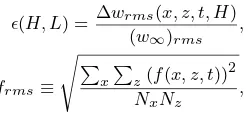
Although the above choiceNs= 2Ntfor RAD2 is physically

realistic, it is interesting to examine how the response depends

upon the ratioNs/Nt(withNs/Nt= 1corresponding to RAD1).

For a 60 min pulse of heating, withL= 10km, Nt= 0.01s−1

and a range of values of Ns, we have computed the upward

energy flux, pw, at the tropopause z=Ht at a fixed time of

t= 60mins. We denote the horizontal average ofpwover 100 km

by qz. This is shown in figure 9. As expected, the upwards

radiation is maximised when Ns=Nt, i.e., when there is no

wave reflection at the tropopause, consistent with the results

of Sutherland (1996; 2010), who considered the simple case of

Boussinesq monochromatic waves in an unbounded atmosphere.

When Ns6=Nt, figure 9 shows that the upwards radiation (in

energy) is reduced by up to 12% over 0.5< Ns/Nt<2. This

reduction is consistent with the results shown in figure 6.

3.4. Triggering of Convection

The triggering of convection is controlled by boundary-layer

thermals having enough kinetic energy to overcome convective

Figure 6.Response att= 60mins to a pulsed heating of lengthT= 30mins, withL= 10km,Nt= 0.01s−1, Ns= 0.02s−1(RAD2 only), andH= 640km

(RAD1, RAD2).

-0.05 -0.025 0 0.025 0.05

< w >

trop

(ms

-1) (a)

t = 30mins

-400 -200 0 200 400 x (km)

-0.05 -0.025 0 0.025 0.05

(b)

t = 60mins

-0.05 -0.025 0 0.025 0.05

(c)

t = 90mins

-400 -200 0 200 400 x (km)

-0.05 -0.025 0 0.025

0.05 Steady Heating

(d)

t = 120mins

(e)

t = 90mins

-400 -200 0 200 400 x (km)

Pulsed Heating

(f)

t = 120mins

-0.25 -0.125 0 0.125 0.25

<

θ

>trop

(K)

-0.25 -0.125 0 0.125 0.25

-0.25 -0.125 0 0.125 0.25

-0.25 -0.125 0 0.125 0.25

Figure 7.Vertically averaged response for steady heating (left) and a 60 min pulse

of heating (right), in RAD1. Shown are vertical averages over the troposphere forw

(blue lines) andθ(red lines), withL= 10km, uniformN= 0.01s−1_{, andH=}

640km. Panels (a,b) show the response to heating over0< t < T = 60mins

(same for both steady and pulsed heating). Panels (c, d) show the response for a further 60 mins of (steady) heating. Panels (e, f) show the response when the heating is terminated after 60 mins (pulsed heating).

Figure 8.Vertically-averaged response for the results of figure 6. Shown are the

vertical averages over the troposphere forw(blue lines) and θ(red lines) at

t= 60mins, to a 30 min heat pulse. Solid lines: TRAP. Dashed lines: RAD1.

Dotted lines: RAD2 (Nt= 0.01s−1,Ns= 0.02s−1)

.

2000), and one process that can erode the CIN is low-level

ascent. This acts to raise the height of any inversion at the top

of the boundary layer, and can also induce convergence that

Figure 9.Horizontally-averaged vertical energy flux|qz|=|pw|, at a fixed time

t= 60min, plotted as a function of ratioNs/Nt, measured with our model RAD2

in response to a 60 min pulse of heating withL= 10km,Nt= 0.01s−1. The

horizontal averaging is done over0< x <100km. Values have been normalised

by the maximum value ofqzacross all values ofNs/Nt.

level subsidence acts to stabilise the troposphere, reducing the

amount of CAPE.

After a localised convection event of the type modelled

here by the prescribed heating, radiating gravity waves provide

the necessary local dynamical adjustment (Bretherton and

Smolarkiewicz 1989), which involves periods of both tropospheric

descent and ascent (figure 6). The initial subsidence pulse with

deep tropospheric warming provides an ambient atmosphere with

reduced CAPE (i.e., less favourable for further convection), but

this disappears in the following pulse, which also has

low-level ascent (to erode CIN, and is thus favourable for further

convection). Case studies have shown these processes to be

influential in controlling the triggering of further convection close

to a parent storm (e.g., Marsham and Parker 2006, Birch et al.

2013), even whenwis only of the order of centimetres per second,

and is thus too small to act as a direct trigger for convection.

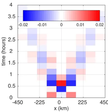
We now use our model to identify zones where the radiating

gravity waves provide an ambient atmosphere favourable for

triggering of convection, in the above sense. Figure 10 shows

results from RAD2 following a 1 h pulse of heating. We consider

θ in the middle troposphere (shown as coloured contours) as a

measure of reduced CAPE, and positivewat 1 km as a measure

of CIN erosion (shown as shaded regions). Immediately after the

termination of heating at 1 h, a series of zones appear with small

or negative mid-troposphericθand positive low-levelw, each of

which moves away from the parent storm and is favourable for

further convection. The first such zone is highlighted within the

dashed contour; this moves outwards from the parent storm at

approximately 20m s−1.

Hello

-500 -400 -300 -200 -100 0 100 200 300 400 500

x (km) 0

1 2 3 4

t (hrs)

Figure 10.Hovm¨oller plot showing the response to a 1 hr pulse of heating in RAD2, withL= 10km,Nt= 0.01s−1,Ns= 0.02s−1. The coloured contours show

mid-troposphericθ; red regions, in which the atmosphere is warmed, will have

reduced CAPE. The shaded region show wherew >0at 1 km, which will act to

erode CIN. The dashed contour encloses one of several bands that may thus be preferential for triggering of subsequent storms.

4. Implications for Convection Parameterisation Schemes

and GCMs

In§3 we quantified the dynamical response to buoyancy forcing

representing a single convection event with a width of about

10 km. We now investigate how the dynamical response to such

an event would appear in a coarse model (e.g., a GCM) in

which convection is not resolved, and is instead parametrised by

applying heating over a grid cell with width of about 100 km. We

consider how the local and remote responses are then altered, and

the implied changes in the heating tendency.

Note that we are not considering the alternative scenario in

which a population of sub-grid clouds (each of width 10 km, say)

is spread over a grid cell of width 100 km (say). In that case,

by a population of small-scale heatings) and that due to a single

smeared-out heating (perhaps corresponding to a convection

scheme) might be smaller. Our experiment, involving a single

isolated sub-grid cloud, might be regarded as a “worst case

scenario” for a convection scheme.

4.1. Sensitivity of Gravity Wave Response to Horizontal Length

Scale of Heating

Under conditions of identical total (x-integrated) heat input, our

model shows that variation in the horizontal length scale of

the heating, L, induces significant changes in the timing and

magnitude of the immediate and remote atmospheric adjustment.

We now quantify these differences for the response to pulsed

heating of duration 1 h, between cases withL= 10km, andL=

100km. The former is representative of single, isolated convective

hot towers, whilst the latter is representative of parameterised

convection in a GCM, where small length scales cannot be

resolved and the heating must be imposed at the grid scale

(or larger). To ensure the same total heat input in both cases,

the maximum buoyancy forcing,S0 satisfies S0(L= 10km) =

10S0(L= 100km).

Figure 11 shows the responses in w and θ. The response is

averaged both vertically over the troposphere0≤z≤10km, and

horizontally over |x−x0| ≤50km for each of x0= 0 (panel

a: local response directly over heating) andx0= 100km (panel

b: remote response). The horizontal averaging means we are

comparing the response to “real” convection (L= 10km) when

smeared over a GCM grid cell of width 100 km, with the response

to parameterised convection (L= 100km) over the same grid cell.

That is, we compare how the responseshouldappear on the model

grid, with how itwillappear when convection is parameterised

(ignoring any additional degradation due to the numerical scheme

of the GCM, since the response here is calculated exactly via (16)

and (17)).

We first discuss the local response shown in figure 11(a). When

L= 10km, thewresponse quickly reaches a steady-state value,

but this “correct” value is never attained whenL= 100km, with

wremaining smaller. It is a similar story for theθresponse, butθ

does eventually reach the “correct” steady-state value. When the

heating is terminated at 1 hr, bothwandθdecay in about 30 mins

whenL= 10km; but the decay takes twice as long (circa 1 h)

whenL= 100km.

The remote response is shown in figure 11(b). Here the

magnitude of the response is smaller whenL= 100km than when

L= 10km, for bothwandθ. There is also a non-trivial change

in the timing of the peak warming, which occurs too soon (by

about 15 mins) whenL= 100km. However, the eventual decay

(fort >2h) is similar in both cases.

There are implications for the accuracy of the entire dynamical

adjustment in GCMs when small-scale convective heating (L=

10km) is replaced by smeared-out parametrised heating on the

grid scale (L= 100km). In particular, this induces errors of about

20% in magnitude in bothwandθ, for both the local and remote

responses. Any dynamical processes sensitive to w and θ will

be correspondingly compromised. For example, the suppression

and initiation of further convection will be modified, via the

CAPE and CIN mechanisms discussed in§3.4. We stress that such

modifications are possible even though the absolute differences in

ware only1−2 cm s−1: these differences would be insignificant for direct triggering of convection, but they will imply 20%

differences in quantities such as CAPE and CIN.

-0.02 0 0.02 0.04

<w>

100km

(m/s)

100km box average

(a)

-0.1 0 0.1 0.2

<

θ

> 100km

(K)

0 1 2 3

t (hrs)

-0.02 0 0.02 0.04

<w>

100km

(m/s)

100km remote box average

(b)

-0.1 0 0.1 0.2

<

θ

> 100km

(K)

Figure 11.Time evolution of the averaged tropospheric responses in RAD2 when

L= 10km (solid lines) andL= 100km (dotted lines). Shown arew(blue) and

θ(red), with additional horizontal averaging over (a)−50km< x <50km (local response) and (b)50km< x <150km (remote response).

Looking at figure 11, one might conclude that, despite

differences in the first few hours after initiation, both cases of

heating are in some agreement by around 3 hours. However,

figure 12, which is an instantaneous vertical cross section of

the vertical structure. Here, ∆w≡(w(L= 100km)−w(L=

10km))and∆θ≡(θ(L= 100km)−θ(L= 10km)).

In summary, from figures 11 and 12 we conclude that narrow,

intense heating, representing a convective hot tower, induces the

largest velocities and warming. Less intuitive is the observation

that the differences in behaviour persist for several hours. Coarse

GCM models with parameterised heating will fail to resolve

some of the variation in responses and, hence, fail to simulate

modification of the convective environment.

Note that the results of this section can also be interpreted

in a completely different way, in which we are comparing the

dynamical responses induced by two fundamentally different

kinds of convection. Then, the narrow intense heating (L=

10km) models a single isolated hot tower, whilst the wider less

intense heating (L= 100km) models a mesoscale convective

system.

4.2. Redistribution of heating

GCM parameterisation schemes generally make the assumption

that all subsidence happens within the convecting grid box

(Arakawa and Schubert 1974) . In this section we estimate the

error associated with the spatial homogenisation (or

smoothing-out) of the grid-box heating (implicit in a GCM) by comparing

adjustments with more realistic heating distributions. Once again,

we will consider the “worst case scenario” where convective

heating in the grid box is confined to a single hot tower.

An appreciation of the error associated with GCM-like

smoothing of heating can be achieved through analysis of the

heating tendency field,∂b_∂t. From (1) recall: ∂b

∂t =S−N

2

(z)w. (37)

For steady heating (which allows a constant value ofbto develop

at all positions in the domain), in the long-time limit, a

steady-state ∂b_∂t = 0develops, when there is a balance between heating andwresponse fields, withS(x, z, t)−N2(z)w(x, z, t) = 0.

To consider the dynamics of tendency in the context of GCMs,

it is first necessary to ensure that all heating is contained within

the spatial domain of our model. For the purposes of this section

(alone) we therefore re-define thex-dependence in our buoyancy

forcing function,S(x, z, t), to be a simple box function

X(x) = Θ

x+L 2

−Θ

x−L₂

, (38)

where, recallΘis the Heaviside function. Whilst the Gaussianx

-dependence used elsewhere in this study is more realistic, a box

function has no tail, and therefore all heating is contained within

the domain which, for present purposes, we regard equivalent to

a parent grid box. We shall consider two cases. The horizontal

heating variation,X(x), is taken to have i) a realistic horizontal

scale withL= 10km, representative of a single cloud, and ii) a

GCM-like smoothed scale withL= 100km. In both cases, the

total heating is ensured to be the same by settingS0(L= 10km)=

10S0(L= 100km). This choice ofX(x)may be straightforwardly

implemented in (16) forw, and then in (20) forb, withGtaken as

G(cj, L, x, t) = Θ(ct−x+L)(ct−x+L)/L (39)

− Θ(ct−x−L)(ct−x−L)/L

− Θ(−ct−x+L)(−ct−x+L)/L

+ Θ(−ct−x−L)(−ct−x−L)/L.

Figure 13 compares the instantaneous spatial integral (inxand

z) of tropospheric heating tendency over a100km box (centred

onx= 0) for our chosen cases (i) and (ii) above. The differences

between the red and blue lines represents the error introduced

when there is smoothing of heating. Shown also is the heating

tendency time series of a scaled heating (black line), which we

shall discuss later in this section.

In the L= 10km heating case, the propagating modes of

subsidence take time to propagate outside the100km box. Thus

for a small time almost all the subsidence is within the box,

and the average tendency,< ∂b/∂t >, is almost constant. As the

descending modes move through the edges of the100km box,

subsidence transfers to neighbouring regions and the tendency

within the box falls. In contrast, when the heating is artificially

smoothed over the 100km box (red line), the subsidence

immediately occurs outside the box and tendency is immediately

reduced inside the parent box, as the vertical motion begins to

L = 10km

w

10

7.5

5

2.5

z (km)

-0.04 -0.02 0 0.02 0.04

θ

0 200 400 600 800

x (km)

7.5

5

2.5

0

z (km)

-0.2 0 0.2

L = 100km

w

-0.04 -0.02 0 0.02 0.04

θ

0 200 400 600 800

x (km)

-0.2 0 0.2

Difference

w

-0.01 0 0.01

θ

0 200 400 600 800

x (km)

-0.05 0 0.05

Figure 12.Vertical cross sections ofw(ms−1_{) andθ(K) response to forcing of horizontal lengthsL= 10km (top) andL= 100km (bottom), which is pulsed for}

t= 1hr. The response att= 4hrs is shown. The right hand column is the difference. Total heating is the same in both cases.

blue line sinks below the red, and it approaches equilibrium faster

than its smooth counterpart thereafter. This behaviour is consistent

with the longer tendency modes in the smoothed heating taking

more time to separate-out and to leave the parent box.

0 15 30 45 60 75 90

time (mins)

-0.02 0 0.02 0.04 0.06 0.08 0.1 0.12 0.14

dbdt (m s

-3 )

10km forcing 10km forcing scaled 100km forcing

Figure 13.Time series of 100 km spatially integrated heating tendencies for a 10 km realistic heating (blue), a 100 km smoothed GCM-like heating (red) and a scaled 100 km heating (black). Total heating is the same in both cases. The difference between the red and blue lines represents a time-local error in heating tendency which arises as a consequence of spatial smoothing of heating, over the domain (GCM box). The black line shows a scaled heating (see text) which has a reduced error in the parent grid box.

A further comparison is made in figure 14, which shows

Hovm¨oller plots of the difference between tropospheric heating

tendency for the cases (i) and (ii) described above. Shown is

a high-resolution solution, in which heating is considered to be

structured within the GCM box, and the same solution coarsened

to GCM-like resolution (∆x= 100km,∆t= 15mins) via spatial

and temporal box averaging. Again we observe subsidence modes

warming neighbouring grid boxes immediately in the smooth

case, and the heating tendency persisting in the parent grid box

for longer. The parent grid box is therefore too cold for the first

30 mins and too warm for the subsequent 30 mins, with errors of

the order of10%apparent. The adjacent grid boxes mirror these

differences for the first hour. Differences in the following hour are

attributed to the longer modes generated from the smooth heating

dispersing the envelope of dominant response (the narrow heating

has a tighter envelope). Differences in the parent and adjacent grid

box after 2hours are minimal (this fact is also visible in figure

13). The domain far-field response shows minimal difference

throughout the simulation.

The errors apparent in figures 13 and 14 suggest a calibration

might fruitfully be applied to GCM heating parameterisation

schemes, to compensate for the thermodynamic errors associated

with incorrect propagation of the subsidence response away

from heating. We postulate a simple multiplicative scaling to

the smoothed GCM-like heating, designed to produce a response

closer to that observed in a calculation forced with a more realistic

(i.e. narrow) horizontal variation of heating. Put another way, we

propose to scale the time-dependence of the forcing in such a

way that the red line in figure 13 moves closer to the blue line.

Accordingly, comparing the smoothed heating with the narrow,

Figure 14.Hovm¨oller plot of differences in tropospheric heating tendency (m s−3_{) between the non-scaled cases considered in figure 13. Panel (a) shows a fully resolved}

solution, panel (b) shows a solution which has been coarsened to 100 km grid box and 15 min time step (representative of a GCM). In the parent grid box, the smoothed heating is too cold at 30 mins, then too warm for 30 mins, before reconciling with the realistic case.

amplitude for some time, followed by a decreased amplitude,

before returning back to its original amplitude for later times,

when the responses to smooth and narrow forcing have reconciled.

Denote the first time at which the lines in figure 13 cross byT1and

that at which both reach equilibrium byT2. For0< t < T1, we

scale the heat-forcing by factorα1>1, forT1< t < T2we scale

it byα2<1, and fort > T2no scaling is applied i.e. we return

the buoyancy forcing to its nominal value.

We now seek to minimise the area between the red and blue

curves of figure 13. We apply the following practical constraints:

1. T1, T2 are chosen to be multiples of 15minute blocks.

From inspection of figures (13) and (14), we chooseT1=

30mins,T2= 60mins.

2. (α1−1)T1= (1−α2)T2 =⇒ α2=T1+T2T−2α1T1.

Constraint 2 is chosen to ensure that total heat input is the same in

both the scaled and non-scaled cases fort > T2.

Using an overall cost parameter,ξ, defined as

ξ=

*

∂b(1) ∂t

x,z

−

∂b(2) ∂t

x,z

+

t

, (40)

whereb(1)is the buoyancy response to aL= 10km forcing and

b(2) is the buoyancy response to aL= 100km forcing, and the

averaging is done over the troposphere in the central 100 km

box. We measure the error, and minimise it over1< α2<1.5.

We find an initial forcing amplification of α1= 1.15 and then

a forcing suppression ofα2= 0.85. The black line in figure 13

shows data from our time-variant scaled smooth heating, which is

now closer to the blue in the parent grid box. However, whilst our

scalingansatzmay improve the response in the parent grid box,

the response in the adjacent field shows the expected increase in

error, as shown in figure 15.

Figure 15.Hovm¨oller plot of differences in buoyancy tendency (m s−3_{) between a}

10km forcing and a100km forcing which has been scaled in order to reduce error

(see text). The parent box now has a reduced error to begin, but the far field has an increased error.

In this section, we have quantified error associated with the

smoothing-out of convective heating in a manner similar to that

performed in GCM-models. We have proposed a mechanism to

improve the grid-box response, with a simple time-dependent

heating parameterisation. Whilst this parameterisation led to error

reduction in the parent grid box, the adjacent and neighbouring

to improve the parameterisation, with more sophisticated

time-dependent heating remains an open question not addressed here.

Certainly, one place to start would be with a more rigorous

analysis of the parameter space influencing the error, together with

consideration of a global error.

5. Conclusion

Using an analytical solution to a 2D thermally-forced, deep

atmosphere, we have constructed an idealised model of convective

adjustment. We have expressed vertical velocity and potential

temperature response in terms of convectively-forced gravity

wave modes and, hence, we have illuminated the role of these

modes in conditioning the troposphere for further convection.

We find that the characteristics of our forced gravity waves are

influenced by the spatial and temporal dependence of the forcing

function, the nature of the upper boundary condition applied to the

domain, and upon model stratification.

We tested the influence of the upper boundary condition and

found that a trapped solution with rigid lid at the tropopause

(allowing no wave radiation into the stratosphere), yields a single

gravity mode, communicating high intensity downward motion

and warming, which propagates into the neighbouring troposphere

and inhibits the chance of further convection. Raising the altitude

of the upper lid high into the mesosphere and beyond (to

approximate the semi-infinite solution) allows a range of

higher-order gravity wave modes to be excited, with much deeper and

faster modes acquiring importance. The convective adjustment is

therefore communicated into the immediate environment faster

than in the trapped case. We note also that allowing waves to

radiate upward sees a reduction in the magnitude and intensity

of the tropospheric response, as expected.

Investigating the temporal dependence of gravity wave

characteristics through a pulsed forcing function, we find that

when the pulse of forcing is truncated, a rebound mode of upward

motion propagates away from the initially heated region, and

the potential temperature response returns to base state. Further,

using figure 10, we identify propagating zones where the radiating

gravity waves provide an ambient atmosphere favourable for

further convection. In such zones, there is no longer tropospheric

subsidence (which reduces CAPE), and there is low-level ascent

which will erode CIN.

The inclusion of a model stratosphere, with Ns= 2Nt

increases the intensity of the tropospheric response, due to wave

reflection at the tropopause. We also notice a slight increase in the

propagation speed of the mode of dominant response. We find a

maximum of energy radiated into the stratosphere (communicated

by gravity waves) for Nt=Ns, as there is no interface and

therefore no reflection. With this in mind, we consider our

trapped model (TRAP) and optimally-radiating model (RAD1) as

respective lower and upper bounds on radiation at the tropopause.

The most realistic intermediate model (RAD2, withNt= 2Ns),

which has partial trapping and radiation, has upward radiation

between the two bounds.

We quantify the error associated with smoothing out convective

heating from a subgrid, single convective hot tower onto a

coarse GCM grid. Performing “worst case scenario” experiments,

in which a convection scheme spreads heating from a cloud

of width 10 km over a full model grid box of width 100 km,

we find that the timing and magnitude of the adjustment is

dependent on the heating distribution. Perturbations in potential

temperature and vertical velocity will be distributed faster and

over a larger region in the parameterised case. Furthermore, an

isolated cloud has a strong response on a sub-GCM-grid scale,

which has implications for the forcing of neighbouring grid cells

in current numerical models, since the timing and magnitude

of the response, communicated by gravity waves, is sensitive

to the horizontal length scale of the forcing function. Further,

analysis of the heating tendency reveals errors of the order of

20% and correspond to a grid-box heating tendency which falls

too quickly when heating is spatially smoothed (parameterised),

due to a failure to account for the finite time taken by small-scale

responses to propagate out of the grid-box. We propose a simple

time-varying scaling to the heating to minimise these errors. Such

a scaling decreases the error in the grid box that is the parent

to convection, but increases error in adjacent boxes. We propose

ways in which to potentially improve this scaling, but leave this

for another study.

The analytical model developed in this work allows us to