Networks: A Stochastic Geometric Framework Based on Cluster Processes
.
White Rose Research Online URL for this paper:
http://eprints.whiterose.ac.uk/131153/
Version: Accepted Version
Article:
Hayajneh, AM, Zaidi, SAR, McLernon, DC orcid.org/0000-0002-5163-1975 et al. (2 more
authors) (2018) Performance Analysis of UAV Enabled Disaster Recovery Networks: A
Stochastic Geometric Framework Based on Cluster Processes. IEEE Access, 6. pp.
26215-26230. ISSN 2169-3536
https://doi.org/10.1109/ACCESS.2018.2835638
© 2018 IEEE. Personal use of this material is permitted. Permission from IEEE must be
obtained for all other uses, in any current or future media, including reprinting/republishing
this material for advertising or promotional purposes, creating new collective works, for
resale or redistribution to servers or lists, or reuse of any copyrighted component of this
work in other works.
[email protected] https://eprints.whiterose.ac.uk/
Reuse
Items deposited in White Rose Research Online are protected by copyright, with all rights reserved unless indicated otherwise. They may be downloaded and/or printed for private study, or other acts as permitted by national copyright laws. The publisher or other rights holders may allow further reproduction and re-use of the full text version. This is indicated by the licence information on the White Rose Research Online record for the item.
Takedown
If you consider content in White Rose Research Online to be in breach of UK law, please notify us by
Digital Object Identifier 10.1109/ACCESS.2018.DOI
Performance Analysis of UAV Enabled
Disaster Recovery Networks: A
Stochastic Geometric Framework based
on Cluster Processes
A. M. HAYAJNEH1,2(Student, IEEE), S. A. R. ZAIDI1(Member, IEEE), DES. C. MCLERNON1 (Member, IEEE), M. DI RENZO3(Senior, IEEE) and M. GHOGHO3,1 (Fellow, IEEE)
1
School of Electronic and Electrical Engineering, University of Leeds, Leeds LS2 9JT, United Kingdom, E-mails: {elamh,s.a.zaidi,d.c.mclernon,m.ghogho}@leeds.ac.uk
2
Department of Electrical Engineering, the Hashemite University, Zarqa, Jordan.
3
The International University of Rabat, TICLab, Morocco.
4
The Laboratoire des Signaux et Systèmes, CNRS, Centrale Supélec, Univ Paris Sud, Université Paris-Saclay, 3 rue Joliot Curie, Plateau du Moulon, 91192 Gif-sur-Yvette, France, E-mail: [email protected].
Corresponding author: A. M. Hayajneh (e-mail: [email protected]).
This work was partly funded by the Hashemite University (HU), Zarqa, Jordan. This work was also partly supported by the UK British Council (Newton Fund) through the Project “Wireless Sensor Networks for Real Time Monitoring of Water Quality” under Grant IL3264631003.
ABSTRACT In this article, we develop a comprehensive statistical framework to characterize and model large scale unmanned aerial vehicle (UAV) enabled post-disaster recovery cellular networks. In the case of natural or man-made disasters, the cellular network is vulnerable to destruction resulting in coverage voids or coverage holes. Drone-based small cellular networks (DSCNs) can be rapidly deployed to fill such coverage voids. Due to capacity and back-hauling limitations on drone small cells (DSCs) each coverage hole requires a multitude of DSCs to meet the shortfall coverage at a desired quality-of-service (QoS). Moreover, ground users also tend to cluster in hot-spots in a post-disaster scenario. Motivated by this fact, we consider clustered deployment of DSCs around the site of a destroyed BS. Joint consideration partially operating BSs and deployed DSCs yields a unique topology for such public safety networks. Borrowing tools from stochastic geometry, we develop a statistical framework to quantify the down-link performance of a DSCN. Our proposed clustering mechanism extends the traditional Matern and Thomas cluster processes to a more general case where cluster size is dependent upon the size of the coverage hole. We then employ the newly developed framework to find closed-form expressions (later verified by Monte-Carlo simulations) to quantify the coverage probability, area spectral efficiency (ASE) and the energy efficiency (EE) for the down-link mobile user. Finally, we explore several design parameters (for both of the adopted cluster processes) that address optimal deployment of the network (i.e., number of drones per cluster, drone altitudes and transmit power ratio between the traditional surviving base stations and the drone base stations).
INDEX TERMS Drones, Stochastic geometry, Unmanned aerial vehicles, Coverage probability, Poisson cluster processes.
A. MOTIVATION
I
N the recent past, we have envisioned an exponential pro-liferation of low-cost embedded systems. These low-cost hardware platforms naturally complement a new breed of software systems provisioned via mobile cloud computing. Effectively, these developments have transformed theyear. With the lower adaptation barrier, drone or so-called unmanned aerial vehicles (UAVs) have attracted significant interest for various applications in the context of smart city solutions. Public safety communication networks are one such application. Rapid on-demand deployment of UAVs furnished with cellular radio platforms is ideal for realizing disaster recovery networks, especially in both rural and urban areas. Consequently, several recent research investiga-tions [1]–[7] have examined the design of a comprehensive framework for the optimal deployment and commissioning of UAVs to enable resilience in public safety networks.
From a communication networks perspective, resilience translates into obliviousness under various failures or asym-metric resource distributions. Specifically, in the context of cellular networks, base station failures can be caused by either a natural or a man-made phenomenon. Natural phenomena such as earthquakes or flooding can result in either destruction of communication hardware or disruption of energy supply to base stations (BSs). Man-made destruc-tion can be either due to a certain sub-system failure or alternatively due to vandalism. In such cases, there is a UAV enabled cellular deployment to present a mechanism through which capacity short-fall can be met in a rapid manner. Drone empowered small cellular networks (DSCNs) present an attractive solution as they can be swiftly deployed for provisioning public safety networks. The ability to self-organize, either in stand-alone or via remote configuration in an on-demand manner, makes the flying cellular network a key enabler for resilient communication networks.
Despite several recent efforts [3], [8]–[11], the design and deployment of flying cells as a disaster recovery network has not been extensively investigated in the literature. The key difficulty is the absence of accurate models for post-disaster operational cellular infrastructure and user distribu-tion. Nevertheless, some specific attributes of post-disaster systems such as surviving user clustering are well known in the existing literature [12]. These attributes can be accom-modated in a stochastic geometric framework to provide system level understanding of DSCNs empowered public safety networks. To this end, we present cluster processes based on stochastic geometric framework for exploring the design space of DSCNs. Noticing that the classical cluster processes do not cater for randomness in the cluster size (which is a key attribute of post-disaster cellular networks), we develop a novel Steinen cell [13], [14] based cluster process model. The model is employed to investigate the design space of DSCNs and several important insights are presented. To the best of the authors’ knowledge, this is the first study to employ the proposed random clustering model to evaluate the design space for future DSCN deployments.
B. RELATED WORK
In the recent past, public safety networking has received significant attention within the third generation partnership project (3GPP) standardization. 3GPP is currently in the process of standardizing proximity services (ProSe) via
Device-to-Device (D2D) communication. The central idea behind ProSe is to form an ad-hoc network where certain nodes of the network (which may still have access to an operational cellular infrastructure in a post-disaster situa-tion) can act as gateways to extend network coverage to isolated nodes. While D2D communication is a promising solution for public safety networks, there are several design challenges which need to be addressed to realize practical deployment with optimal design parameters. In particular, in multi-hop D2D communication networks, those nodes which are connected to the cellular network may become traffic-forwarding hot-spots. Due to limited battery capacity of mobile user equipment, traffic hot-spots may reduce the operational life-time of the entire network. Moreover, the network in its essence is ad-hoc and thus guaranteeing reliable connectivity is not possible. That is, a network operator controlled solution is the best approach to optimally deploy such networks.
Despite the growing popularity of the aforementioned, DSCNs present an attractive alternative and complementary deployment option. That is, drones can offer many posi-tives to overcome the typical ad-hoc networks problems: (i) they present fast and resilient deployment, (ii) they can be controlled via a centralized network operator to increase compatibility and interoperability, and (iii) the propagation conditions are much more favourable and can be further optimized by exploiting controlled mobility of the drones. Consequently, it is envisioned that both D2D and DSCNs will complement the legacy private/professional mobile radio (PMR) (e.g., trans- European trunked radio (TETRA) and project 25 (P25)) for enabling next generation public safety networks [15]–[17]. In the recent past, many researchers are trying to define an optimal deployment framework for such networks. Indeed, there are two main approaches. The first is the one focusing on constructing an analytical framework to build the optimal network even by counting the intrinsic randomness or assuming a fixed network structure [18]–[20]. The second approach deal with building optimal algorithms to define the deployment geom-etry parameters in an efficient manner [21]–[25]. However, within these two direction, we will focus on building an analytical statistical framework to study the randomness of the network by harnessing stochastic geometry tools in a user-centric fashion in contrast to the popular whole network performance coverage averaging studies.
Relying on the results of link budget and path-loss model, the DSCNs can be designed and optimized in the same way as in the 5G heterogeneous networks. However, the differences are in the capabilities of the drone base stations (DBSs) in terms of capacity and airtime etc. To this end, some studies were conducted to measure the prospective performance enhancement and to identify the design imple-mentation conditions and elements of operation. Here, many researchers tried to find the optimal drone 3D placement which secures the maximum coverage for single or multiple drones working in a recovery constrained area [2], [19].
In our previous work in [19], we studied the coverage probability for a constrained recovery area where the de-struction is assumed to be in a small circular region of the space. However, this is not the case for a whole network performance short-fall recovery. Hence, we introduce the cluster based recovery network structure.
The new structure of DSCNs leads to several new deploy-ment topologies. For instance, cluster based fixed ground IoT networks have been addressed in [25]. In this study, an optimal clustering given the limited capacity for every UAV is investigated. Essentially, the optimal deployment of DSCNs is an application dependent problem. That is, for IoT and WSN applications, we need to define how many clusters we need to deploy while assuming that one UAV is only needed to serve each cluster. However, for a post-disaster scenario where a cellular BS is destroyed, demands for clustered users cannot be satisfied through a single UAV. The optimal network dimensioning considering the number of drones deployed per cluster thus becomes a design question. To this end, we will introduce the user-centric deployment geometry where each cluster is served by multiple UAVs. Our stochastic framework is built on following key attributes.
BS station destruction model: To model a post-disaster cellular network, we consider that BSs are independently destroyed with a certain probability. Consequently, employ-ing the widely used Poisson point process (PPP) model for the original cellular network implies that a post-disaster network can be modeled via a thinned point process. The independent thinning model for post-disaster networks is widely adopted as in [3], [9]–[11]. Extension of this model to a scenario where BS destruction probability incorporates spatial correlation is more involved and may obscure some design insights. This aspect will be tackled in a future work. Cluster based user and UAV deployment model: In or-der to model clustering between users in a post-disaster scenario, we extend the traditional Neyman-Scott cluster processes [26]. In [27]–[31] cluster processes have been employed to model user-centric heterogeneous cellular net-works. In particular, Poisson cluster processes (PCP) such as the Matern’s cluster process (MCP) and the Thomas cluster process (TCP) are employed to model locations of small cellular networks. Nevertheless, our analysis significantly differs from these existing works in two aspects; (i) in the existing literature, cluster processes which model small cellular networks are considered along with the PPP which models the underlying macro cellular network. However, in the context of disaster recovery networks the clusters are only created on dead spots (i.e., destroyed BSs). Conse-quently, this will result into a mixture model where (ii) the cluster size for a small cellular network is a design parameter. However, for a disaster recovery network, the cluster size is related to the coverage area of the desired de-stroyed cell site. Therefore, the cluster size itself is a random variable. These two factors are explicitly accommodated in our analysis. A mathematical analysis is presented in Section
II.
Cluster size model: As mentioned before, one of the key features of the resultant topology for a DSCN based public safety network is that there exists a one-to-one mapping between the coverage area of destroyed the BS and the size of a cluster of UAV small cells deployed to meet the short-fall. Considering the strongest average received power based association cellular networks, association regions form a Voronoi tessellation. Consequently, for a post-disaster sce-nario, a Voronoi cell of a destroyed BS needs to be replaced with a cluster of UAVs. The cluster size is a function of the area of the Voronoi cell which itself is a random quantity. Also, the geometrical approximation of area for mapping is intricate. In this regards, [13], [14] have shown that the area of the Stienen cell, i.e. a circular inscribing-disc formed at the location of the destroyed BS with respect to its distance to the nearest neighbour, is an adequate proxy for the size of the Voronoi cell. Consequently, we consider clusters have random radii where the radius distribution corresponds to the Stienen cell [13], [14]. Vertical back-hauling/front-hauling: In order to complete the design of the recovery network, we need to highlight the back-haul design1. Generally, the
back-haul literature can be classified into two parts. The first type of studies, focus on the 3D placement for a back-haul aware drone based communication network while the other studies explore enabling technologies for back-hauling such as mmWave, FSO etc. The 3D placement of the back-haul aware networks is studied in [22]. Authors in [22] addressed the network design and limiting factors for user-centric and network-centric topologies. Nevertheless, analytical model for performance quantification has not been developed as the study was geared towards back-haul design. The work also highlights the key limitations for adopting various back-haul technologies. The enabling technologies for the vertical back-hauling/front-hauling have been addressed in several papers in the literature. In [7], the authors presented the use of free space optics (FSO) as a promising technology enabler in future 5G+ wireless networks. Authors in [7] demonstrated that FSO is capable to deliver data rates higher than the baseline wireless and wired alternatives. However, FSO is highly sensitive to weather conditions and the back-haul capacity may dramatically decrease in foggy weather. The proposed solution to this drawback is developed via in-band backhauling. That is, using the current LTE, WiFi or even the HSPA radio frequency microwave links can be considered as good solutions for faster interoperability and cost effectiveness. However, this will result in more degradation of the quality of service (QoS) due to the extra interference from aggressive frequency reuse. Finally, the design of the network back-haul is totally dependent on the type of service that operator aims to deliver. In many scenarios, especially in post disasters, coverage is the main
1Here, we only highlight some of the advances made on back-hauling
key performance metric and hence high data rates may not be the aim of the network operator. In this case, multi-hop relaying for coverage extension can be the fastest and a cost effective solution [32].
C. CONTRIBUTION & ORGANIZATION
To summarize, the key contributions and organization of this paper are as follows:
1) We develop a comprehensive statistical model for quantifying the coverage, area spectral efficiency, and energy efficiency of DSCNs for post disaster recovery. To the best of our knowledge, the underlying topology yields a point process which has not been considered before even in the stochastic geometric literature. 2) Borrowing tools from stochastic geometry, we present
a statistical framework for quantifying the perfor-mance of large scale DSCNs deployment considering two types of cluster networks with different scenar-ios for the deployment geometry. Also, the analyti-cal framework is subsequently employed for design optimization answering the following questions (see section III):
a) Is there an optimal cluster size to achieve an optimal coverage and throughput performance? b) Considering the optimal cluster size chosen, is
there any optimal location for the drone small-cells and the number of drones in every cluster in a way to maximize the performance metrics? c) How does the variable cluster size change
com-pared to fixing the size of all the clusters? d) How does changing the power ratios change
the energy efficiency performance of the whole network? (see section IV).
3) Finally, some critical design issues are explored and possible future developments are summarized (see section VII).
D. NOTATION.
Throughout this paper, we employ the following mathe-matical notations. The counting measure of a point process Φ(B)provides a count of points inside the compact closed subset B ∈R2 (i.e., bounded area). The probability density function (PDF) for a random variable X is represented as fX(x) with the cumulative density function written as
FX(x). The exclusion symbol \ represents the exclusion of a subset from a superset. The expectation of a function
g(X)of a random variableX is represented asEX[g(X)]. The bold-face lower case letters (e.g., x) are employed to denote a vector in R2 andkxk is its Euclidean norm. The Laplace transform (LT) of any random variableZ isLZ(s) (i.e., LT of the PDF of the random variable).
I. NETWORK AND PROPAGATION MODEL A. DEPLOYMENT GEOMETRY
Spatial Model for a Post-disaster Cellular Network:Similar to [19], [27], [33], we consider a large scale macro-cellular
network where the locations of the BSs are modelled by a homogeneous PPP (HPPP) (Φ) such that
Φ ={x0, x1, ..., x∞,∀ xi∈R2} with intensityλ. (1) Coverage holes in post-disaster result from the destruction of the cellular infrastructure. These coverage holes are mod-elled by location independent thinning ofΦwith probability of thinning po 2
. Hence, the survived macro base stations (MBSs) will be modeled by a thinned HPPP [34] such that
ΦS ={x∈Φ :1(x) = 1} with intensityλS =psλ,(2) where 1(.) denotes a Bernoulli random variable3. Notice
that the thinning process results in a new HPPP ΦS which has intensity λS such that λS = (1−po)λ =psλ, where
ps is the BS survival probability. Consequently, the HPPP of destroyed BSs is given by
ΦD= Φ\ΦS, (3)
which has an intensity of λD = poλ. The point process ΦD, which preserves the number and the location of the holes, will then be used to model the location and number of points around which the DSCs are deployed to fill the coverage hole.
Network Model for DSCN: In order to fill the coverage holes after the thinning process, it is assumed thatNdDSCs, also called daughter points, are deployed as replacements for each destroyed BS in ΦS. The key motivation behind deployment of multiple DBSs to fill the coverage hole created by a destroyed MBS pertains to the limitation on the capacity of the DBSs as well as the difference in transmission power and radio prorogation conditions as compared to the MBSs. Consequently, the resulting network geometry is modelled with two collocated point process, the former for the operational survival MBSs (denoted by ΦS) while the later is for the DBSs (denoted byΦD). The location of DCSs can be modelled by a general Neyman-Scott process [26]. This type of Poisson clustered process is formed by simply distributing a finite number of daughter points (Nd) around the parent pointx∈ΦD. The resulting point process is then the union of all the daughter points by preserving their locations around the parent points without including the parent points themselves. The union of all the DSCs in the space around the parent point processΦD(i.e., destroyed BSs) will form a clustered process which can be defined as
ΦC
∆
= [
i∈{0,1,...,n−1}
{ΦCi+xi},∀xi∈ΦD, (4)
where ΦCi is a cluster with Nd DCSs such that ΦCi =
{y1, ..., yNd,∀ yi ∈ R
2}, n is the number of the parent
2We adopted the uniform independent thinning for the sack of simplicity
and the lack of any actual physical model for the destruction resulting from natural or man-made occurrences.
3Note that the Bernoulli random variable1(x) is independent of the
locationx. However,xis only used as a location preserving parameter to preserve the original location of the holes.
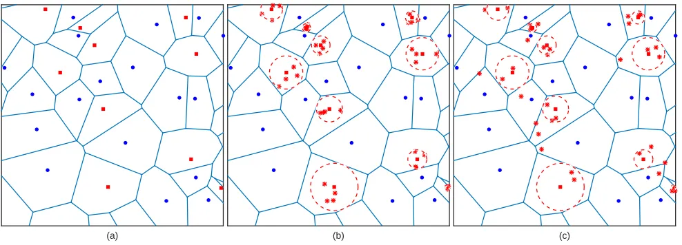
(a) (b) (c)
FIGURE 1: (a) Traditional cellular network where some MBSs are destroyed with probabilitypo= 0.3. (b) Four DBSs are distributed uniformly in the two dimensional space around the center of every destroyed MBS according to a MCP model as in (5). (c) Four DBSs are distributed normally in the two dimensional space around the center of every destroyed MBS according to a TCP model as in (7). Blue circles, red squares and red stars are the retained MBSs, destroyed MBSs and the deployed DBS, respectively. A dashed circle is the radius of the deployment recovery area around the destroyed MBS.
points in ΦD and xi is the location of the ith point in R2. Also, the clusters in ΦC, without loss of generality, are divided into two sets of clusters: (i) the one called the representative cluster contains the set of all points around x0 (a typical destroyed BS) and is defined by
ΦCin
∆
= ΦC0, and (ii) the set of all cluster process points except the points in the representative cluster and is defined byΦCout
∆
= ΦC\ΦC04.
The distribution of the daughter points around the cluster center defines the type of the cluster process (see Figure 1). Accordingly, we will study two types of cluster process where the DBSs are spatially distributed as follows:
1) Matern’s Cluster Process (MCP): In a Matern’s cluster process (MCP), a fixed numberNd points are distributed uniformly in the two dimensional space according to the density function
fM(x) = 1
πσ2
M
, kxk ≤σM, (5) whereσM is the radius of the cluster. Then, the PDF of the distanceR from any point in the cluster to the parent point follows the uniform distribution
fM R (r) =
2r σ2
M
. (6)
2) Thomas Cluster Process (TCP):In a Thomas cluster process the set of cluster points (DBSs) are normally
4We also denoteΦ
Cx = ΦCi to denote the cluster around the parent pointxi ∈ΦD. Moreover, wherever M orT subscripts or superscripts appear, this means that the symbol is related to Matern’s and Thomas cluster processes, respectively (as defined in subsequent discussion).
distributed in the two dimensional spaceR2according to the density function
fT(x) = 1 2πσ2
T
exp −kxk
2
2σ2
T
!
, (7)
whereσT is the standard deviation and represents the scattering distance around the origin of the axis. Thus, the PDF of the distanceRfrom any point in the cluster to the parent point follows the Rayleigh distribution5
fT R(r) =
r σ2
T
exp − r
2
2σ2
T
!
. (8)
In this paper, we assume that the typical drone mobile user (DMU) is located in the destruction zone and is always associated to the nearest DBS6. We also assume that, the
probability of being associated to a MBS is very low since the distance to the nearest DBS is absolutely lower than the distance to the nearest MBS (i.e., the nearest DBS provides the highest average signal strength).Here, the assumption is accurate due to the adoption of cluster based distributions of the users and DBSs. Similarly, the authors in [28] show that this assumption is accurate even for the “maximum power association” scheme which is more sensitive for fading and network tier transmit power ratios. Clearly, the user is more likely to be served by its cluster centre if the distribution is more dense around the cluster centre. In our model, this is more likely to be accurate since we are using the nearest
5This follows from the joint transformation of f
x=(X,Y)(x, y) to
f(R,Θ)(r, θ)and then taking the marginal distribution of the distanceR.
6With slight abuse of notations, we use DMU to denote to a typical user
[image:6.576.42.536.70.248.2]base station association. In addition, the large scale model for the sky to ground channel is much favourable as regards providing line of sight links with higher received SIR at the user antenna.
Spatial Model for DMUs: It is assumed that the distri-bution of the users around the center of the clusters is the same as the DBSs with the same density. This follows from the fact that every DBS is associated to only one user in the same channel resource block. Hence, we mapΦC7→ΦDMUC for the set of the users around cluster centers with density
λC7→NdλDMUC .
B. PROPAGATION MODEL
Large Scale fading Model: In order to accurately capture the propagation conditions in a DSCN, we employ the path-loss model presented in [3]. The employed path-path-loss model adequately captures line of sight (LoS) and non line of sight (NLoS) contributions for drone-to-ground communication as follows:
lLoS(h, r) =KLoS−1
r2+h2−
α 2
, (9)
lN LoS(h, r) =KN LoS−1
r2+h2−
α 2
, (10) whereh is the height of the drone in meters,r is the two dimensional projection separation between the drone and the DMU,KLoSandKN LoSare environment and frequency dependent parameters such thatKi=ζi c/(4πfM Hz)
−1
,
ζiis the excess path-loss fori∈ {LoS, N LoS}with typical values for urban areas (ζLoS = 1 dB,ζN LoS = 20dB)and
α= 2is the path-loss exponent for free space path-loss (see [3] for details). The probability of having a LoS link from the DSC for the desired DMU is as follows:
PLoS(θ) =
1
1 +a1e−b1η θ+b1a1
, (11a)
PN LoS(θ) = 1− PLoS(θ), (11b) wherea1,b1,c1 are environment dependent constants,η=
180/πandθis the elevation angle in degrees. Consequently, we define the total average excess path-loss as
¯
κ(r) =KN LoS+
K∆
1 +a1e−b1ηtan−
1(h r)+b1a1
, (12) whereK∆=KLoS−KN LoS, andr=h/tan(θ). Note that, the average path-loss from the DBS to the desired DMU can be quantified from the above equations as
¯
ld(r) = ¯κ−1(r)(r2+h2)−1. (13) The large scale path-loss for the down-link of the cellular network is modelled by the well-known power law path-loss function
lS(r) =K−1r−α. (14) whereα, the path-loss exponent has typical values between 2 and 4. K is the excess path-loss and has typical values
between 100 dB and 150 dB (see [35], [36] for details). This simple power law path-loss model is widely adopted in literature for analysis of large scale cellular networks and has been used here to simplify the analysis as we are only studying the link for the DSC associated DMU.To conclude, the large scale path-loss for the sky-to-ground channels is modelled by a single slope model with different values for the excess path-loss for the LoS and NLoS with path-loss exponentα= 2. For the ground-to-ground channels we use a single model for both LoS and NLoS with the path-loss exponentα= 3.5. This is due to the fact that the surviving base stations are all seen as interferers and are more likely to be in NLoS with the user which is assumed to be served by the nearest DBS.
Small scale Fading: It is assumed that large-scale path-loss for both of the traditional cellular-link and the DCSs is complemented with small-scale Rayleigh fading such that
|g|2∼Exp(1). Also, it is assumed that the network is operat-ing in an interference limited regime (i.e., performance of all links is dependent upon co-channel interference and thermal noise at the receiver front-end is negligible). The assumption of a Rayleigh fading model is due to simplicity of analysis. This assumption will not compromise our results, since Rayleigh fading implicitly gives a worst-case analysis of the Nakagami-m fading channel where (i.e., m = 1 no LoS component). However, the effect of LoS and NLoS components is incorporated in the large scale fading model given by (12).
C. TRANSMISSION MODEL
In this paper, we assume that the DMU is associated to nearest DBS (i.e., the BS which maximizes the average received signal to interference ratio (SIR)) and transmitters on the same frequency are considered as co-channel inter-ferers. These out-of-cell interferers can be classified into three categories: (i) the interference received from MBSs working on the same channel as the serving DBSs, (ii) the interference from the set of DBSs located inside the representative cluster and called “intra-cluster interferers”, and (iii) the interferers from out of the representative cluster and called “inter-cluster interferers”.
Remark 1. To complete the transmission model, we assume that the average number N¯d of co-channel active DBSs inside any of the clusters has a Poisson distribution which is also related to the number of channel resources used (Nc) such thatN¯d= NNdc.
II. DISTANCE DISTRIBUTIONS
In this section, we characterize link distance distributions which are required to quantify the large scale path-loss given by (13). These distributions are employed to quantify coverage probability in section III.
A. DISTRIBUTION OF THE RADIUS OF THE RECOVERY AREA
In order to tackle the way of distributing the DSCs in the network we will study two types of cluster processes: (i) the traditional cluster process, where the standard deviationσi is fixed for all of the clusters and (ii) the modified Stienen’s cell model. In the later process, the standard deviation (i.e., the recovery cell radius) is considered to be the same as the radius of the Stienen’s cell. This comes from the fact that the destroyed base stations will act as holes as defined in (3). Here, the Stenien’s cells are considered the most loaded cells and hence the circular modeling of the recovery area is a good approximation. Note, that for high-dense micro-cellular networks, as within cities, the approximation will be more accurate.
In the light of the above discussion, a good approximation of the recovery cell size can be built around the Steinen’s model with cells of radius σi∀i ∈ {M, T}. Thus, the distribution of the cluster spread in which the DBSs will be deployed is considered to be the distribution of the generalized Stienen’s cell radius, i.e.,
fσi(σi) = 2πλτ σiexp
−πλτ2σ2
i
,∀i∈ {M, T}. (15) Here, setting the value ofτ = 2gives the distribution of the radius of the maximum inscribed circle, centered on the the destroyed MBS location and is equal to half of the distance to the nearest neighbour in the original tessellation which is well known as the Stienen’s cell radius. Tunning the value of τ will tune the radius of the recovery area where the DBSs will be distributed.
B. DISTANCE DISTRIBUTIONS FOR MCP
We now consider the distance distributions assuming that DBSs and DMUs are uniformly distributed around the centers of the destroyed MBSs according to a MCP.
As shown in Figure 2, we consider a typical user at location Vo =kxk from the center of the representative cluster and served by the link to the nearest DBS with a distance R1 =kx−y1k where y1 represents the location
of the nearest DBS. Then to evaluate the distribution of the distance R1, we need to make a random variable
transformation and then apply order statistics rules on the well-known distribution of the DBSs distance R to the cluster center which has the PDF:
fM R (r) =
2r σ2
M
,0≤r≤σM, (16)
and CDF FM
R (r) = r 2 σ2
M,0 ≤ r ≤ σM. We also assume that the distance Vo from the DMU to the cluster center is a random variable with the PDF,
fVMo(vo) = 2vo
σ2
M
,0≤vo≤σM. (17) Then, by performing a joint random variable transfor-mation of fM
R (r) such that the distance D(R, Vo) =
p
V2
o +R2−2VoRcos(θ) is the distance from the DMU at Vo and any arbitrary DBS at distanceR from the center of the cluster andθis the angle between the linesRandVo with the PDFfΘ(θ) =21π,0≤θ≤2π, then the distribution
of the distance R conditioned that DMU is at location Vo will have the PDF (18) with the CDF as in (19) [37].
Next, the distribution of the distanceR1 from the typical
DMU and the nearest DBS can be evaluated as in the next proposition.
Proposition 1. The distribution of the distanceR1from the
typical DMU at Vo and the nearest DBS can be evaluated for MCP as in(20)(on the next page).
Proof. Let,Nd BSs be distributed uniformly inside a circle of radius σM, Then the derivation of the nearest neigh-bour distribution amongst the Nd DBSs follows the order statistics using the fact that for general Nd i.i.d. random variablesZi∈ {Z1, Z2, ..., ZNd}ordered in ascending order with PDFs fZi(z). Then the PDF of Z1 = min
i (Zi) can be written as fZ1(z) = N 1−FZi(z)
N−1
fZi(z) [38]. Then, by applying this to (18), we can write the PDF of the distance R1 as
fM
R1(r1|vo, σM) =
fM R(1)1
(r1|vo, σM), 0≤r1≤σM −vo,
fM R(2)1
(r1|vo, σM), σM−vo< r1≤σM+vo (21)
where
fM
R(1)1 (r1|vo, σM) =Nd(1−F M
R(1)(r1|vo))Nd−1fRM(1)(r1|vo)(22)
fM
R(2)1 (r1|vo, σM) =Nd(1−F M
R(2)(r|vo)) Nd−1
fRM(2)(r1|vo)(23).
From the previous proposition, fM
R1(r1|vo, σM) can be easily integrated in (20) to get the CDF of the nearest neighbour distance distribution as
FR1M(r1|vo, σM) =
(
(1−FM
R(1)(r1|vo, σM))Nd, 0≤r≤σM −vo (1−FM
R(2)(r1|vo, σM))Nd, σM−vo< r≤σM+vo (24)
Proposition 2. The distribution of distance Rx from the in-cluster DBSs interferers to the typical user located at distance Vo from the cluster center (conditioned that the nearest neighbour DBS is at distance R1 with the
distribu-tion in (20)) can be written as in(25).
Proof. The proof of this is simple. Following from the fact that the distance to the nearest interferer is larger than the serving distance R1, then the area of circle formed by
fRM(r|vo, σM) =
fRM(1)(r|vo, σM) =σ2r2 M
, 0≤r≤σM−vo,
fRM(2)(r|vo, σM) =πσ2r2 M
arccos
r2+v2 o−σM2
2vor
, σM−vo < r≤σM+vo
(18)
with the CDF as follows:
FRM(r|vo) =
FM
R(1)(r|vo) = r 2 σ2M
, 0≤r≤σM−vo,
FM
R(2)(r|vo) = r 2 π σ2
M
θ1−12 sin (2θ1)+π1 θ2− 1
2 sin (2θ2)
, σM−vo< r≤σM+vo
(19)
withθ1= arccos
r2−σ2M+vo
2vor
andθ2= arccos
−r2+σ2 M+vo
2voσM
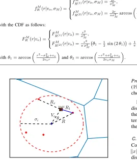
[image:9.576.40.309.65.380.2]. θ σi R1 R Vo Rx DMU
FIGURE 2: Spatial distribution of network elements. Brown square for the DMU. Red circles for DBSs. Red dashed circle is the recovery area. Blue diamond is the center of the Voronoi cell (i.e., Destroyed BS).
truncated from the whole area. Therefore, we can write the conditional distribution of this event as follows:
fM
Rx(rx|vo, σM, r1) =fRM(rx|vo, σM), R > r1
= f
M
R (rx|vo, σM)
R∞ r1 f
M
R (r|vo, σM)dr
= f
M
R(rx|vo, σM) 1−FM
R (r1|vo, σM)
. (26)
Hence, by substitutingfM
R (rx|vo, σM)andFRM(r1|vo, σM) into (25) we complete the proof.
Following from the above proposition, we can easily show that the distribution of distances from the DMU atVoto the out-of-cluster interferers can be evaluated for a MCP as in the next proposition.
Proposition 3. The PDF of the distance distribution from the typical user at distanceVofrom the cluster center to the interfering DBSs from out of the representative cluster can be written for MCP as
fRMo(ro|u, σM) =f M
R (ro|u, σM). (27)
Proof. The proof of this follows the same steps to evaluate (19) by doing the joint transformation for the uniformly chosen DBS - see also [27].
In the previous proposition, we assumed that the relative distances from the cluster DBSs to any typical DMU inside the cluster is independently identical amongst all the clus-ters. Hence, we will use shifted versions of (27) to complete the coverage probability analysis (see(40)) [26].
C. DISTANCE DISTRIBUTIONS FOR TCP
Conditioning on the typical user located at distance Vo =
kxk from the cluster center we can write the PDF of the distribution of distance from any arbitrary chosen drone to the typical user at vo for TCP as [27]:
fT
R(r|vo, σT) =
r σ2
T
exp−r
2+v2
o 2σ2
T Io rvo σ2 T ! ,(28)
and the CDF as:
FT
R(r|vo, σT) = 1−Q1
vo σT , r σT . (29) The distanceVofrom the DMU to the cluster center is also a random variable with the PDF,
fT Vo(vo) =
1
σ2
T
exp − v
2
o 2σ2
T
!
. (30)
The nearest neighbour DBS to the typical user located at distance Vo from the center of the cluster can be evaluated as follows in the next proposition.
Proposition 4. The PDF of the distanceR1from the typical
user at a distanceVo from the cluster center to the nearest DBSs for TCP can be evaluated as
fT
R1(r1|vo, σT) =
Ndr1
σ2
T
exp−r
2 1+vo2
2σ2
T
Io
r1vo
σ2
T
!
× Q1
vo
σT
, r1 σT
!Nd−1 (31)
where Q1
vo σT,
r σT
is the Marcum Q-function, and
Io rvo σ2 T
is the first kind Bessel function .
fM
R1(r1|vo, σM) =
fM R(1)1
(r1|vo, σM) =2Nσ2dr1 M
1− r21 σ2 M
Nd−1
, 0≤r1≤σM −vo,
fM R(2)1
(r1|vo, σM) =2πσNd2r1 M arccos
r2 1+v2o−σ2M
2vor1
× 1−
r21 π σ2
M
θ1
1−12 sin 2θ11
+π1θ1
2−12 sin 2θ21
!
Nd−1
, σM −vo< r1≤σM +vo (20) withθ11= arccos
r12−σM2+vo
2vor1
andθ21= arccos
−
r12+σM2+vo
2voσM
.
fM
Rx(rx|vo, σM, r1) =
2rx σ2
M−r21, 0≤rx≤σM −vo, 2rx
πσ2 M
arccos
r2 x+v2o−σ2M
2vo rx
1− r 2 1 π σ2 M
θ1
1−12 sin(2θ 1 1) −1 π θ1
2−12 sin(2θ 1 2)
, σM −vo< rx≤σM+vo.
(25)
Proof. This can be evaluated by assuming that the number of drones (Nd) per cluster is fixed and using the ordered statistics of the distance distribution of the cluster DBSs points to the typical user located at distance Vo from the center of the cluster.
In the next proposition we show the distribution of the distance from the in-cluster interferers and the typical DMU.
Proposition 5. The distribution of distance Rx from the in-cluster DBSs interferers to the typical user located at distance Vo from the cluster center (conditioned that the nearest neighbour DBS is at distanceR1 with the
distribu-tion in (31)) can be written as
fT
Rx(r|vo, σT, r1) =
rx σ2
T exp
−r2x+v 2 o
2σ2 T
Io
rxvo σ2 T Q1 vo σT,
r1 σT
.(32)
Proof. The proof follows the same steps as in (26)
Following the above proposition, we can easily show that the distribution of distances from the typical user at Vo to the out-of-cluster interferers can be evaluated for TCP as in the next proposition.
Proposition 6. The PDF of the distance distribution Ro from the typical user at distance vo from the cluster center to the interfering DBSs out of the representative cluster can be written for TCP as
fT
Ro(ro|u, σT) =
ro
σ2
T
exp−r
2
o+u2 2σ2
T
Io
rou
σ2
T
!
.(33)
Proof. Proof follows the same steps as in Proposition 3.
III. COVERAGE PROBABILITY
In order to characterize the link level performance of DSCNs, we employ coverage probability as a metric. The coverage probability of an arbitrary user is defined as the
probability at which the received signal-to-interference-ratio (SIRi) is larger than a pre-defined thresholdβ such that 7
Pi
c =Pr{SIRi≥β}, i∈ {M, T}. (34) Then, considering that both of the DBS and the MBS networks are sharing the same channel resources, the SIRi can be quantified as:
SIRi= PD|g|
2¯
ld(r1)
IΦi Cin+IΦ
i
Cout +IΦS
= PD|g|
2¯
ld(r1)
Ii tot
, i∈ {M, T}.
(35)
where
IΦi Cin =
X
y∈Φi Cin
PD|g|2
h2+kx 0+yk2
−1
¯
κ kx0+yk
| {z }
In-cluster interference
IΦi Cout =
X
x∈Φi D\x0
X
y∈Φi Cx
PD|g|2
h2+kx+yk2−1
¯
κ kx+yk
| {z }
Out-of-cluster intereference
IΦS =
X
x∈ΦS
PS|g|
2
lS(kxk)
| {z }
Interference from survival BSs
. (36)
Here r1 represents the distance from the DMU to the
nearest DBS;|g|2is the channel power gain coefficient and it is assumed to be the same for all the links;IΦi
Cin represents the received interference from the DBSs in the representative cluster; IΦi
Cout represents the received interference from the co-channel DBSs concurrently transmitting with the
7The network is assumed to be operating in an interference limited
considered representative link from out of the cluster; IΦS is the interference received from the retained MBSs; and
PS andPD are the transmit power for the MBS and DBS respectively.
Consequently, the coverage probability can be evaluated as
Pis
c = Pr{SIRi s
≥β},
= Pr{|g|2≥Itoti βκ¯(r1)
r21+h2
/PD},
(a)
= Er1,σi
h
EIi tot
h
exp−sIi tot
ii
,
(b)
= Er1,σi
LIΦi Cin
(s|r1, σi)LIΦi Cout
(s|r1, σi)LIΦS(s)
(37)
where s = β r2 1+h2
¯
κ(r1)/PD, (a) is obtained by
averaging over the channel coefficient and (b) is obtained by applying the definition of the Laplace transform then using the addition property of the Laplace transformation of independent random variables.
Next, we introduce the coverage probability for DMU under the two deployment topologies rendered via MCP and TCP.
A. COVERAGE PROBABILITY FOR MCP
To complete the analysis of the coverage probability, we need to quantify the Laplace transformations for the interfer-ence at the typical DMU. In the next lemma, we introduce the Laplace transform of the distribution of the in-cluster interference for the MCP.
Lemma 1. The Laplace transform of the interference at the DMU from the in-cluster DBSs for MCP can be evaluated as
LIΦM Cin
(s|r1, σM) = Nd
X
i=1
Z ∞
r1
fM
Rx(rx|vo, σM) 1 + sPD
¯
κ(rx)(h2+r2x) drx
i−1
×ξ(i, Nd), (38)
where
ξ(i, Nd) = ¯
Ni
dexp(−N¯d)
i!ΣNd k=1
¯
Nk
dexp(−N¯d) k!
. (39)
Proof. Please refer to Appendix A.
In order to complete the analysis of the coverage proba-bility, we also need to derive the Laplace transform of the interference from out-of-cluster DBSs (see Lemma 2).
Lemma 2. The Laplace transform of the interference distri-bution at the DMU from out-of-cluster DBSs for MCP can be evaluated as in(40).
Proof. Please refer to Appendix B.
B. COVERAGE PROBABILITY FOR TCP
For the sake of comparative analysis, the Laplace transform of the distribution of the in-cluster interference for TCP, can be obtained in the following Lemma.
Lemma 3. The Laplace transform of the interference at the DMU from the in-cluster DBSs for TCP can be evaluated as:
LIΦT Cin
(s|r1, σT) = Nd
X
i=1
Z ∞
r1
fRTx(rx|vo, σT) 1 + sPD
¯
κ(rx)(h2+r2x) drx
i−1
×ξ(i, Nd). (41)
Proof. Please refer to Appendix C.
Lemma 4. The Laplace transform of the interference dis-tribution at the DMU from out-of-cluster DBSs for TCP can be evaluated as in(42)
Proof. Please refer to Appendix D.
The Laplace transform of the interference from the re-tained MBSs is calculated in Lemma 5. In this Lemma, we will relax the dependency of the drone network parent points and the location of the retained base stations. In other words, we will relax the dependency of location between the retained MBSs and the typical DMU. This relaxation is compulsory; since the distribution of the distance between the retained MBSs and the desired DMU is not known for correlated BSs and DMUs locations. Moreover, this assumption is assumed to be close to the true value since we are averaging over the random user location atVowhich will average to a location at the location of the parent point (i.e., the destroyed BS), and this is valid for both the MCP and TCP topologies. An insight into the accuracy of this assumption is shown in Figure 3. The figure shows the CDF of a distance Dfrom the typical DMU atVo to the nearest neighbour retained MBS.
Lemma 5. The Laplace transform of the interference distri-bution at the drone typical user from the retained MBSs with density λS = (1−po)λcan be approximated as follows:
LIΦS
(s) = exp−πλS Nc
s−2 αP−
2 α S sinc α2
(43)
where s=β r2 1+h2
¯
κ(r1)/PD.
Proof. The proof of this is straight forward from the Laplace transform of the PPP and can be illustrated as follows:
LIΦ S
(s) = E(exp(−sIΦS)), = E(exp(−s X
x∈ΦS
PS|g|
2
lS(kxk))),
= EΦS
Y
x∈ΦS E|g|2
exp−s|g|2lS(kxk) ,
(a)
= exp−2πλS
Z ∞
0
sPSKS−1r−α+1 1 +sPSKS−1r−α
dr,
LIΦM Cout
(s|σM) = exp
−2πλD
Z ∞
0
1−exp−Nd
Nc
Z ∞
0
1− 1
1 +sPDκ¯(u)(h2+u2)
fM
Ro(u|v, σM)du
vdv. (40)
LIΦT Cout
(s|σT) = exp
−2πλD
Z ∞
0
1−exp−Nd
Nc
Z ∞
0
1− 1
1 +sPDκ¯(u)(h2+u2)
fT
Ro(u|v, σT)du
vdv. (42)
d
0 500 1000 1500 2000 2500 3000 3500
C
D
F
0 0.2 0.4 0.6 0.8 1
[image:12.576.38.278.582.701.2]po ={.3, .5, .7}
FIGURE 3: Nearest MBS distribution CDF for TCP. λ= 1×10⁻⁶. Dashed line for Monte-Carlo simulation. Solid
line for the relaxed distance distribution FD(d) = 1− exp(−πλSd2).
(b)
= exp−2πλS Nc
s−2 αP−
2 α S sinc α2
(44)
where (a) is obtained by applying the expectation over the fading channel coefficient assuming i.i.d. Rayleigh channels followed by the probability generating functional (PGFL) of the PPP of the Rayleigh distribution and then followed by Cartesian to polar transformation and then solving the integration to get (b) which completes the proof.
Theorem 1. The coverage probability of a typical DMU with fixed recovery cell radius σi can be respectively eval-uated for Matern’s and Thomas cluster processes as
PcM(σM) = ∞
Z
0 ∞
Z
0 LI
ΦMCout(s|r1, σM)LIΦM Cin
(s|r1, σM)LIΦS(s)
×fRM1(r1)f M
Vo(vo) dr1dvo, (45) and
PcT(σT) = ∞
Z
0 ∞
Z
0 LIΦT
Cout
(s|r1, σT)LIΦT Cin
(s|r1, σT)LIΦS(s)
×fRT1(r1)f T
Vo(vo) dr1dvo. (46)
Theorem 2. The coverage probability of a typical DMU with variable recovery area cell radius σi can be
respec-tively evaluated for Matern’s and Thomas cluster processes as.
PMs c =
∞ Z
0
PM
c (σM)fσM(σM) dσM, (47) and
PTs c =
∞ Z
0
PcT(σT)fσT(σT) dσT, (48)
where the superscript s denotes to the fact that the coverage probability will be averaged over the Stienen’s cell radius. Next, we will use the coverage probability results above to quantify area spectral and energy efficiencies.
IV. AREA SPECTRAL EFFICIENCY AND ENERGY EFFICIENCY
Until now, we have studied the coverage probability for the two assumed system models. To study the network level performance, we need to quantify the Area Spectral Efficiency (ASE) of the network given that a channel reuse is assumed. In this section we show analysis of ASE for both the MCP and the TCP.
Proposition 7. Given the coverage probabilities in(47)and (48), the ASE of the network for MCP can be evaluated as
ASEM =λDNdNcPcMslog2(1 +β), (49)
and for TCP as
ASET =λDNdNcPcTslog2(1 +β). (50)
In order for comprehensive study of the network, we also make use of the term energy efficiency (Eef f). The Eef f (in general) can be evaluated as [39]:
Eef f=
Area Spectral Efficiency
Average Network Power Consumption= ASE λDNdPD
. (51)
Given the ASE in (49) and (50), we can evaluate Eef f for MCP as
Eef fM =
NcPcMslog2(1 +β)
PD
, b/J/Hz (52) and for TCP as
ET ef f =
NcPcTslog2(1 +β)
PD
TABLE 1: Simulation parameters.
Parameter Value Description
ζLoS, ζN LoS 1,20 dB Excess path-loss
fM Hz 900 MHz Carrier frequency
α 3.5 Path loss exponent
K 132 dB Excess path-loss for macro cells
a1, b1 9.6,0.28 Environment dependent constants
λ 1×10⁻⁶ Base stations density
Nc 2,1 Available number of channels
PD 1dBW Drone cell transmission power
PS 10dBW MBS cell transmission power
V. RESULTS AND DISCUSSION
In this section, we show numerical results for the coverage probabilities (i.e.,PMs
c andPcTs) and energy efficiency (i.e.,
EM
[image:13.576.298.521.73.263.2]ef f and ETef f) of drone-based communication recovery network deployment. Furthermore, we assume that the DBSs are operating in an urban environment with the parameters shown in Table 1.
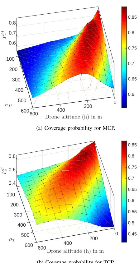
Figure 4 shows the coverage probability of a random uni-formly chosen user inside the recovery area for both MCP and TCP with fixed cluster size (see (45) and (46)). The coverage probability is plotted against both the cluster radius (σi) and the DBSs altitude (h). An interesting observation here is that the drone-based clustered recovery network can achieve a significant enhancement of the coverage probability when the cluster radius is around a certain value and the optimal point changes by changing the height of the drones and vice versa. That is, we will have a unique optimal drone height for every chosen cluster radiusσi. We can notice also that a significant coverage probability can be achieved inside of the clusters with coverage figures up to0.85by only utilizing Nd= 3 drones with one channel. It is worth also to keep in mind that the proposed system is considering a user centric distribution where the location of the drones is coupled with the location of the users where the capacity needs to be extended. This means that these coverage probabilities can be achieved only inside of the circular shaped coverage areas of the recovery cells. Moreover, choosing between MCP and TCP as a framework for the network performance analysis does actually depend on the distribution of the users in the targeted recovery areas (e.g., uniformly for rural areas and normally for high-dense urban areas). This due to the fact that the cellular infrastructure is actually being built towards the user and hence the distribution of the users will define which type of cluster process is more suitable for the recovery network.
Remark 2. For the case of λ = 1×10⁻⁶, the average
optimal cell size is close to 250m which is approximately the same as the Stenien’s cell average radius. That is, the variable cell radius is more realistic and gives an implicit optimal selection of the recovery cell radius.
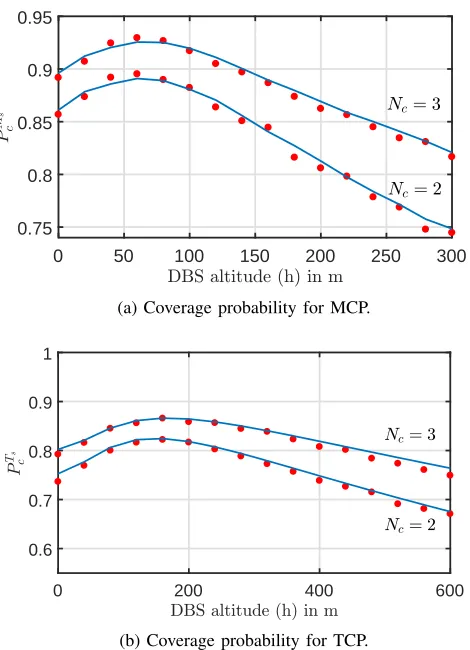
Figure 5 depicts the coverage probability against the altitude of the drones for both of the MCP and TCP where the Stenien’s cell size is deployed (see (47) and (48)). The
P
M c
100 0.6
200
300
σM
400 0.7
500 0
Drone altitude (h) in m
200 400
600 600 0.8
0.6 0.65 0.7 0.75 0.8 0.85
(a) Coverage probability for MCP.
P
T c
0.4
100
200
300
σT
400 0.6
0 500
Drone altitude (h) in m
200 400
600 600 0.8
0.45 0.5 0.55 0.6 0.65 0.7 0.75 0.8 0.85
(b) Coverage probability for TCP.
FIGURE 4: Coverage probability for arbitrary chosen typi-cal user for fixed value of recovery cell radiusσi.Nc= 1,
po= 0.2,λ= 1×10⁻⁶, N
d= 3, α= 3.5, PD/PS = 0.2 andβ =−5 dB.
[image:13.576.44.268.75.176.2]coverage probability shows that for a thinning probability of 0.1, with 5 drones deployed in every cluster, the optimal drone altitude will slightly change as increasing the number of channels and this will intuitively increase the coverage probability. For example, for TCP, there is an optimal altitude difference of 30m when increasing the number of channels from 2 to 3. This existence of an optimal drone altitude which maximizes the coverage probability is due to the adoption of LoS/NLoS model for the large scale path-loss model which is widely addressed in the literature of stochastic geometry [2], [33], [40].
Figure 6 shows the coverage probability plotted against the number of drones per cluster for multiple configuration
0 50 100 150 200 250 300 0.75
0.8 0.85 0.9 0.95
(a) Coverage probability for MCP.
0 200 400 600
0.6 0.7 0.8 0.9 1
[image:14.576.306.535.68.402.2](b) Coverage probability for TCP.
FIGURE 5: Coverage probability for an arbitrarily chosen DMU for Stenien’s recovery for MCP and TCP (see (47) and (48)). Original MBS and DMU densities isλ= 1×10⁻⁶.
The destruction probabilitypo= 0.1.α= 3.5.N
d = 5.and
PD/PS = 0.2. Blue solid lines for the exact solution and the red dots for the Monte-Carlo simulation.
of transmit power ratios for both of MCP and TCP where the Stenien’s cell size is deployed (see (47) and (48)). The coverage probability curves show that, for a fixed transmit power ratio, there is an optimal number of drones at which the higher densification of the clusters will not increase the coverage probability. For example, for the configuration where the ratio PD/PS = 1%, we need only 3 drones to achieve the optimal coverage. This is an interesting result which is contrary to the idea of densification of the heteroge-neous networks. The main reason for this phenomenon is the adoption of the LoS/NLoS 3D model for large scale fading. This can be further justified as illustrated in [41]. In this paper, the authors showed that the densification under the 3GPP path-loss models with variable base station elevation will change the behaviour of the network performance metrics with regard to the change of the density of the deployed base stations. That is, for any chosen network density of base stations, there is an optimal density of base stations that gives the optimal coverage probability as well
2 4 6 8 10
0.6 0.7 0.8 0.9
(a) Coverage probability for MCP.
2 4 6 8 10
0.6 0.65 0.7 0.75 0.8
[image:14.576.40.275.71.396.2](b) Coverage probability for TCP.
FIGURE 6: Original MBSs density is λ= 1×10⁻⁶. The
destruction probability po = 0.1. α = 3.5 and P
D/PS =
{1,2,3,4} ×10−2.
as the optimal ASE. In addition, the base stations density which maximizes the achievable coverage probability will differ from the one which maximizes the ASE.
Figure 7 showsEef f plotted against the number of drones per cluster for multiple configuration of transmit power ratios for both the MCP and TCP where the Stenien’s cell size is deployed (see (52) and (53)). No value of an optimal number of drones can be seen for the case of energy efficiency. That is, as we increase the number of the drones we increase the network throughput. Moreover, the trend of the energy efficiency is to increase as we increase the transmit power ratio.
VI. FUTURE WORK
1 2 3 4 5 6 7 8 9 10 0 1 2 3 4 5
FIGURE 7: Energy efficiency vs. the number of drones per cluster. Original MBSs density is λ = 1 ×10⁻⁶.
The destruction probability po = 0.1. α = 3.5. and
PD/PS ={1,2,3,4} ×10−2.
effective distribution of the drones, an estimation of the location of the users and the number of hot-spots required is necessary. This will lead to an estimation problem of the optimal number of drones to be used and the location of clusters (i.e., hot-spots) where the drones need to be distributed. A good solution for an efficient estimation of the number and location of clusters, is to utilize a real-time k-mean clustering relying on a drone enabled users’ localization scheme.
In this work, we assumed independent thinning of BSs. Actually, this assumption is sufficient for the sake of sim-plifying the analysis. However, this might be non-realistic for urban areas of the city. In some post disaster scenarios (e.g., earthquakes or human made destruction), the thinning process might be dependent on the geographical location of the BS. Hence, a comprehensive mathematical modelling of the thinning process can be more accurate and give a better performance insight.
Lastly, the developed framework can also be extended to incorporate Massive MIMO base station. From interference management perspective this will present completely new dynamics.
VII. CONCLUSION
In this paper, we introduced a statistical and analytical framework for evaluating the coverage probability and en-ergy efficiency performance metrics for cluster based drones enabled recovery networks. Results show that there are a number of parameters which influence optimal deployment of the recovery network: (i) number of drones in a cluster, (ii) drone altitudes, (iii) transmission power ratio between drone base stations and traditional base stations, and (iv) the recovery area radius. Furthermore, it is also shown that by optimizing these parameters the coverage probability and the energy efficiency of a ground user can be significantly enhanced in a post-disaster situation.
APPENDIX A PROOF OF LEMMA 1
The Laplace transform of the interference from in-cluster DBSs at a typical DMU can be evaluated for a MCP as
LIΦM Cin
(s|r1, σM) (a)
=
Ehexp−s X
y∈ΦM Cin
PD|g|2
h2+kx0+yk2
−1
¯
κ kx0+yk
i
(b)
=Eh Y y∈ΦM Cin
1 1 +sPD¯ 1
κ(kx0+yk)(h2+kx0+yk2)
i (c) = Nd X i=1 Z ∞ r1 1 1 + sPD
¯
κ(kx0+yk)(h2+kx0+yk2)
fM(y) dy
i−1
× N¯
i
dexp(−N¯d)
i!ΣNd
k=1 ¯ Nk
dexp(−N¯d)
k!
| {z }
ξ(i,Nd)
(d) = Nd X i=1 Z ∞ r1 1 1 + sPD
¯
κ(rx)(h2+r2 x)
fRMx(rx|vo, σM) drx
i−1
×ξ(i, Nd). (54)
where (a) is obtained by applying the definition of the Laplace transform,(b)is obtained by taking the expectation over the Rayleigh fading channel coefficient |g|2, (c) is obtained by applying the PGFL and conditioning that the number of co-channel operating drones K =k is Poisson distributed. We include the fact that the total number of co-working drones is less than Nd and, (d) is obtained by a simple change of variableskx0+yk → ro and then by transformation from Cartesian to polar coordinates.
APPENDIX B PROOF OF LEMMA 2
The Laplace transform of the interference from out-of-cluster DBSs at a typical DMU can be evaluated for a MCP as
LIΦM Cout
(s|r1, σM) (a)
=
Ehexp−s X
x∈ΦD\x0
X
y∈ΦM Cx
PD|g|2
h2+kx+yk2−1
¯
κ kx+yk
i
(b) =EΦD
h Y
x∈ΦD\x0
EΦM Cx
h Y
y∈ΦM Cx
1
1 +sPD(
h2+kx+yk2)−1
¯ κ(kx+yk)
ii
(c) =EΦD
h Y
x∈ΦD\x0
exp−Nd
Nc
×
Z ∞
0
1− 1
1 +sPD¯κ(ro)(h12+r2 o)
fRMo(ro|v, σM) dro
i
(d)
= exp−2πλD
Z ∞
0
1−exp−Nd
Nc
Z ∞
0
×1− 1
1 +sPD¯κ(ro)(h12+r2 o)
fRMo(ro|u, σM) dro
udu
(55)
where (a) is obtained by applying the definition of the Laplace transform,(b)is obtained by taking the expectation over the Rayleigh fading channel coefficient|g|2 assuming i.i.d. fading channels,(c)is obtained by applying the PGFL with change of variables kx+yk → ro and then by transformation from Cartesian to polar coordinates, and(d) is obtained by applying the PGFL of the PPP.
APPENDIX C PROOF OF LEMMA 3
The Laplace transform of the interference from in-cluster DBSs at a typical DMU can be evaluated for TCP as
LIΦT Cin
(s|r1, σT) (a)
=
Ehexp−s X
y∈ΦT Cin
PD|g|2
h2+kx 0+yk2
−1
¯
κ kx0+yk
i
(b)
= Eh Y y∈ΦT Cin
1 1 +sPD¯ 1
κ(kx0+yk)(h2+kx0+yk2)
i (c) = Nd X i=1 Z ∞ r1 1 1 + sPD
¯
κ(kx0+yk)(h2+kx0+yk2)
fT(y) dy
i−1
× N¯
i
dexp(−N¯d)
i!ΣNd
k=1 ¯ Nk
dexp(−N¯d)
k!
| {z }
ξ(i,Nd)
(d) = Nd X i=1 Z ∞ r1 1 1 + sPD
¯
κ(rx)(h2+rx2)
fRTx(rx|vo, σT) drx
i−1
×ξ(i, Nd) (56)
where (a) is obtained by applying the definition of the Laplace transform,(b)is obtained by taking the expectation over the Rayleigh fading channel coefficient |g|2 and, (c) is obtained by applying the PGFL and conditioning that the number of co-channel operating drones K =k is Poisson distributed and, (d) is obtained by a simple change of variableskx0+yk → ro and then by transformation from Cartesian to polar.
APPENDIX D PROOF OF LEMMA 4
The Laplace transform of the interference from out-of-cluster DBSs at a typical DMU can be evaluated for TCP as
LIΦT Cout
(s|r1, σT) (a)
=
Ehexp−s X
x∈ΦD\x0
X
y∈ΦT Cx
PD|g|2
h2+kx+yk2−1
¯
κ kx+yk
i
(b) =EΦD
h Y
x∈ΦD\x0
EΦT Cx
h Y
y∈ΦT Cx
1
1 +sPD(
h2+kx+yk2)−1
¯ κ(kx+yk)
ii
(c) =EΦD
h Y
x∈ΦD\x0
exp−Nd
Nc
×
Z ∞
0
1− 1
1 +sPD¯κ(ro)(h12+r2 o)
fRTo(ro|v, σT) dro
i
(d)
= exp−2πλD
Z ∞
0
1−exp−Nd
Nc
Z ∞
0
×1− 1
1 +sPD¯κ(ro)(h12+r2 o)
fRT(ro|u, σT) dro
udu(57)
where (a) is obtained by applying the definition of the Laplace transform,(b)is obtained by taking the expectation over the Rayleigh fading channel coefficient G assuming i.i.d. fading channels,(c)is obtained by applying the PGFL with change of variables kx+yk → ro and then by transformation from Cartesian to polar coordinates and,(d) is obtained by applying the PGFL of the PPP.
REFERENCES
[1] M. Mozaffari, W. Saad, M. Bennis, and M. Debbah, “Unmanned aerial vehicle with underlaid device-to-device communications: Performance and tradeoffs,” arXiv preprint arXiv:1509.01187, 2015.
[2] A. Al-Hourani, S. Kandeepan, and S. Lardner, “Optimal lap altitude for maximum coverage,” Wireless Communications Letters, IEEE, vol. 3, no. 6, pp. 569–572, 2014.
[3] M. Mozaffari, W. Saad, M. Bennis, and M. Debbah, “Drone small cells in the clouds: Design, deployment and performance analysis,” arXiv preprint arXiv:1509.01655, 2015.
[4] S. Rohde, M. Putzke, and C. Wietfeld, “Ad hoc self-healing of ofdma networks using uav-based relays,” Ad Hoc Networks, vol. 11, no. 7, pp. 1893–1906, 2013.
[5] S. Chandrasekharan, K. Gomez, A. Al-Hourani, S. Kandeepan, T. Rasheed, L. Goratti, L. Reynaud, D. Grace, I. Bucaille, T. Wirth, et al., “Designing and implementing future aerial communication networks,” arXiv preprint arXiv:1602.05318, 2016.
[6] X. Li, D. Guo, H. Yin, and G. Wei, “Drone-assisted public safety wireless broadband network,” in Wireless Communications and Networking Con-ference Workshops (WCNCW), 2015 IEEE, pp. 323–328, IEEE, 2015. [7] M. Alzenad, M. Z. Shakir, H. Yanikomeroglu, and M.-S. Alouini,
“Fso-based vertical backhaul/fronthaul framework for 5g+ wireless networks,” [8] A. Merwaday and I. Guvenc, “Uav assisted heterogeneous networks for
public safety communications,” in Wireless Communications and Net-working Conference Workshops (WCNCW), 2015 IEEE, pp. 329–334, IEEE, 2015.
[9] I. Bucaille, S. Hethuin, T. Rasheed, A. Munari, R. Hermenier, and S. Allsopp, “Rapidly deployable network for tactical applications: Aerial base station with opportunistic links for unattended and temporary events absolute example,” in Military Communications Conference, MILCOM IEEE, pp. 1116–1120, IEEE, 2013.
[10] W. Guo, C. Devine, and S. Wang, “Performance analysis of micro un-manned airborne communication relays for cellular networks,” in Com-munication Systems, Networks & Digital Signal Processing (CSNDSP), 2014 9th International Symposium on, pp. 658–663, IEEE, 2014. [11] M. Gharibi, R. Boutaba, and S. L. Waslander, “Internet of drones,” arXiv
preprint arXiv:1601.01289, 2016.
[12] S. Saha, A. Sheldekar, A. Mukherjee, S. Nandi, et al., “Post disaster management using delay tolerant network,” in Recent Trends in Wireless and Mobile Networks, pp. 170–184, Springer, 2011.
[13] R. Hernandez-Aquino, S. A. R. Zaidi, M. Ghogho, D. McLernon, and A. Swami, “Stochastic geometric modeling and analysis of non-uniform two-tier networks: A stienen’s model-based approach,” IEEE Transactions on Wireless Communications, vol. 16, no. 6, pp. 3476–3491, 2017. [14] S. Srinivasa and M. Haenggi, “Distance distributions in finite uniformly
random networks: Theory and applications,” IEEE Transactions on Vehic-ular Technology, vol. 59, no. 2, pp. 940–949, 2010.
[15] X. Lin, J. Andrews, A. Ghosh, and R. Ratasuk, “An overview of 3gpp device-to-device proximity services,” Communications Magazine, IEEE, vol. 52, no. 4, pp. 40–48, 2014.
[16] G. Baldini, S. Karanasios, D. Allen, and F. Vergari, “Survey of wireless communication technologies for public safety,” Communications Surveys & Tutorials, IEEE, vol. 16, no. 2, pp. 619–641, 2014.