This is a repository copy of
Probabilistic sensitivity analysis in cost-effectiveness models:
determining model convergence in cohort models
.
White Rose Research Online URL for this paper:
http://eprints.whiterose.ac.uk/134173/
Version: Accepted Version
Article:
Hatswell, A.J., Bullement, A., Briggs, A. et al. (2 more authors) (2018) Probabilistic
sensitivity analysis in cost-effectiveness models: determining model convergence in cohort
models. Pharmacoeconomics. ISSN 1170-7690
https://doi.org/10.1007/s40273-018-0697-3
The final publication is available at Springer via https://doi.org/10.1007/s40273-018-0697-3
[email protected] https://eprints.whiterose.ac.uk/
Reuse
Items deposited in White Rose Research Online are protected by copyright, with all rights reserved unless indicated otherwise. They may be downloaded and/or printed for private study, or other acts as permitted by national copyright laws. The publisher or other rights holders may allow further reproduction and re-use of the full text version. This is indicated by the licence information on the White Rose Research Online record for the item.
Takedown
If you consider content in White Rose Research Online to be in breach of UK law, please notify us by
Probabilistic sensitivity analysis in cost-effectiveness models;
Determining model convergence in cohort models
Anthony J. Hatswell1,2, Ash Bullement3, Andrew Briggs4, Mike Paulden5, Matt Stevenson6
1. University College London, London, UK 2. Delta Hat Limited, Nottingham, UK 3. BresMed Health Solutions, Sheffield, UK 4. University of Glasgow, Glasgow, UK 5. University of Alberta, Edmonton, Canada 6. University of Sheffield, Sheffield, UK
Key words: cost-utility; health technology assessment; economic modelling; pharmacoeconomics
Abstract
Probabilistic sensitivity analysis (PSA) demonstrates the parameter uncertainty in a decision problem. The technique involves sampling parameters from their respective distributions (rather than simply using mean/median parameter values). Guidance in the literature, and from HTA bodies, on the number of simulations that should be performed suggests a sufficient number , or until
Key points for decision makers
An arbitrary number of probabilistic simulations may lead to unacceptable variability in results by chance alone known as Monte Carlo error
There are a number of techniques by which model convergence can be assessed, our preferred being the running of the model until the 95% confidence interval for the incremental net monetary benefit does not include zero
1.
Probabilistic sensitivity analysis in health economics
Probabilistic sensitivity analysis (PSA) is a method for accounting for parameter uncertainty in cost-effectiveness models. A distribution is assigned to each parameter, reflecting uncertainty in the true value, accounting where possible for the correlation between parameters. Samples are then
repeatedly drawn from each distribution and used as model inputs. Each unique set of inputs (a ) results in a unique set of model outputs. Considering the results of many simulations allows for estimation of the expected (mean) model outputs and the uncertainty around these outputs [1,2].
PSA is mandated by many health technology assessment (HTA) agencies internationally, including
UK N I H C E NICE) and the Canadian Agency for Drugs and Technologies in Health (CADTH) [3,4]. It is also recommended in guidelines published by the International Society for Pharmacoeconomics and Outcomes Research (ISPOR), and the Society for Medical Decision Making (SMDM) [5]. The reason for this requirement is in non-linear models, results based only on a fixed selection of input values will be biased. Common reasons for this are the use of median values where the median value does not equate to the mean value in the underlying distribution (such as a lognormal distribution) and where the combinations of changing parameters alter the number of patients simulated to experience health states associated with large costs utility impacts . Only through probabilistic analysis can the true results of non-linear models be identified.
To illustrate the importance of using probabilistic analysis, a PSA was conducted using 250,000 simulations in a published model [6] this large number is assumed to give close approximations of
Incremental Cost Effectiveness Ratio (ICER). Whilst the deterministic ICER was £25,961, the probabilistic estimate was £20,684 showing the difference that can occur between the two in non-linear models. This was followed by a series of 20 additional PSAs where for each of this series the mean ICER was calculated separately over simulations 1 to n, for n = 1 to 10,000, allowing for consideration of change in the mean as the number of simulations increases. As the number of simulations increases, the range of the mean ICERs across the series of PSAs narrows (Figure 1).
A ICE‘ ICE‘
20 PSAs but only 12 of 20 had converged to within £250. Running more simulations 17 out of the 20 had converged to within £250 at 5,000, with all 20 having done so by 10,000 simulations.
Common presentations of PSA results include tabulation of mean model outputs and the probability that the intervention is cost-effective at plausible cost-effectiveness thresholds, scatterplots of simulations on the cost-effectiveness plane, cost-effectiveness acceptability curves (CEACs) and frontiers (CEAFs) [7,8]. These allow for consideration of the mean and distribution of model outputs [9] and may be used to inform value of information analysis [10].
Since PSA requires random sampling from distributions the parameter inputs will differ each time the PSA is repeated across equal numbers of simulations, such that the model outputs will also differ. In cohort models (the form of models we address in this tutorial), it follows that there are two uncertainties: the distribution of outputs across simulations within a PSA; and the difference
between mean outputs across PSAs which reflects random noise (i.e. Monte Carlo error). The first type of uncertainty is what PSA aims to estimate, but the second type of uncertainty is undesirable. Fortunately, the greater the number of simulations conducted, the smaller the Monte Carlo error and if this error is sufficiently small, then as the error is considered inconsequential.
the Monte Carlo error, this increases the computational resources required and adds little value if convergence has already been reached. It follows that current practice is problematic: if too few simulations are conducted then the PSA results may incorporate substantial Monte Carlo error; but if too many simulations are conducted then the PSA is computationally inefficient. Without
justification for the analysis performed, it is not possible to know where on this spectrum the analysis lies.
The objective of this tutorial is to consider how model convergence can be considered in practice in cohort models (individual patient models are the topic of a separate literature). The topic is
illustrated using the published example of chondrocyte implantation for cartilage damage of the knee [6].
2.
Potential outcomes of interest
In addition to the complexity of the economic model itself, the number of simulations required for convergence of any given model depends upon the outcomes of interest to the decision maker and the desired level of accuracy for each outcome.
The most commonly considered model output is the ICER, typically the cost per quality-adjusted life year (QALY) gained. If the decision maker requires only an estimate of the mean ICER, the number of simulations should be just sufficient for this statistic to converge. Additional simulations may be required beyond the number required for the ICER statistic to converge if outputs other than the mean ICER are of interest to the decision maker [11,12]. For example, the decision maker may be interested in a confidence interval for the ICER estimate, the -effectiveness falls below a certain threshold, or the expected value of perfect information (EVPI) of an intervention. Alternatively it may be important that the estimated distributions of the model outputs are accurate between PSAs, and not merely the mean ICER alone. This may require additional simulations to ensure convergence towards the edges of each distribution which are inherently less stable than the mean.
An alternative outcome is the incremental net benefit (INMB) statistic, a positive value of which signifies a technology is cost-effective [13,14]. Whilst ICERs may be more frequently used in decision making, the net-benefit statistic has a number of desirable properties compared to the ICER. Most importantly, the moments of its distribution are defined theoretically, such that it is possible to define a variance mathematically, and the assumption of a normal sampling distribution is
reasonable under conditions imposed by the central limit theorem. By contrast, the ICER, as a ratio of two random variables, does not have a mathematically tractable variance.
For these reasons, we focus on net-benefit quantities in this tutorial in order to assess the
convergence of important outcomes for the purposes of cost-effectiveness decision making, while recognising that the analyst may want to convert back to the use of the ICER when presenting the results of their cost-effectiveness analysis.
3.
Appropriate level of accuracy
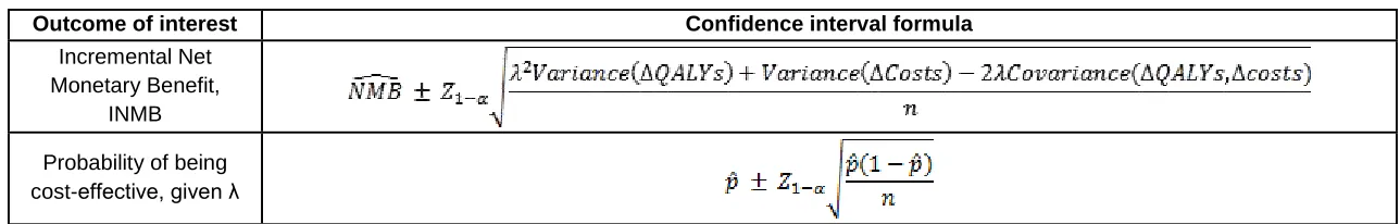
Ideally the decision maker would specify not only the outcomes of interest, but also the desired level of accuracy. This could be defined in terms of standard errors around the mean ICER, or absolute levels of accuracy e.g. ICERs to be reported within a tolerance of ±£500. A further request may also be for the probability an intervention is cost-effective, though in isolation these may be misleading, with funders typically preferring mean ICER [15]. For convenience the formulae for the confidence interval of the INMB and probability of being cost effective at a given threshold are given in Table 1.
4.
Defining convergence
For a linear model, the mean outputs in a
PSA will converge towards these values. It follows that the outputs of interest may be considered to have converged when they have stabilised (given the desired level of accuracy) to the respective deterministic outputs (i.e. the mean ICER has stabilised to within the specified accuracy of the deterministic ICER).
For a non-linear model, the deterministic outputs will values. The values can only be estimated empirically: as the number of simulations increases, the mean outputs in the PSA will converge towards these true values (although by definition, these
. It follows that the outputs of interest may be considered to have converged when they have stabilised sufficiently close to the outputs that would be observed if an infinite number of simulations were to be performed.
Regardless of the model type, each mean output in the PSA will fluctuate as the number of simulations increases, stabilising D period of fluctuation, it is possible for a mean output to remain stable temporarily, or value by chance, only to diverge away as the number of simulations increases. To ensure
convergence, it follows that it is not appropriate to halt a PSA immediately upon observing that a mean output appears stable; more robust methods are required.
In determining convergence, the use of visual aids has been used previously in HTA submissions and journal publications, and can be an effective form of communicating how the level of uncertainty varies [16 18]. However, interpretation of visual aids is subjective and may imply stability (or instability) dependent on the scales of the plot chosen.
Our suggested approach for determining when outputs have converged makes use of the INMB outcome by determining a confidence interval (CI) around the mean outcome. The CI around the point estimate of the INMB can then be translated to a CI around the point estimate of the ICER for presentation to a decision maker by instead of the INMB, calculating the ICER i.e. incremental cost divided by incremental QALY, as opposed to x incremental QALY incremental cost. The choice of significance level will depend on the decision problem, however for simplicity we suggest this should be 5% or less as is current standard convention in the medical field.
INMB is chosen specifically to avoid mathematical limitations of interpreting the uncertainty around the point estimate of a ratio, such as the ICER. The INMB is normally distributed (and therefore its variance is well defined) provided that the incremental costs and QALYs each follow a normal distribution (per the Central Limit Theorem, assuming a large [n>30] number of simulations). The variance around the point estimate of the ICER is undefined, and so convergence of the ICER is not determined directly.
For an adoption decision, if after a given number of simulations the CI of the INMB does not contain zero no further simulations are required i.e. increased precision of the point estimate of the INMB would be very unlikely to change the decision made. Conversely, if the CI still contains zero after a given number of simulations, further simulations would be required to produce a CI that excludes zero. In the case of cohort models which have short computational times this is not anticipated to create a burden apart from a very rare situation where the true ICER was equal to .
For decision makers, the ICER is most frequently used to present the results of cost-effectiveness analysis. As such, it is of interest to be able to present the uncertainty around the ICER itself particularly for decision makers e.g. the Scottish Medicines Consortium [SMC]) or lies within a range (e.g. NICE) [4,19]. The value of at which the INMB is zero represents the point estimate of the ICER. The uncertainty in the INMB can be translated into the uncertainty in the ICER, by identifying the values of at which the lower bound of the INMB is zero and the upper bound of the INMB is zero. These values may be found by trial and error or may be calculated using goal seek functionality within Microsoft Excel, or with similar mathematical programming functions
in other software S R).
5.
Worked example
For our proposed approach, we will consider the number of simulations required for the mean ICER to converge in our example model. The mean ICER should be calculated as the quotient of the mean incremental costs and QALYs over the number of simulations considered (i.e. not the mean of individually-calculated ICERs for each simulation).
F A and
a significance level of 5%, the resultant point estimate and CI of the mean INMB achieved after 500 simulations is -£120 (95% CI: -£687, £447). As this CI includes zero, the conclusion drawn is that a larger number of simulations are required. Increasing the number of simulations to 1,000 yields a result of -£426 (95% CI: -£825, -£27). As this CI no longer contains zero, 1,000 simulations may be considered sufficient in this example as the adoption decision would be unlikely to change should an increased number of simulations be performed.
H I
obtaining an ICER within a maximum tolerance of £500 in either direction. The associated point estimates and 95% CI around the ICER is £20,181 (£19,427, £20,943). Given the width of this CI is greater than £1,000, further iterations would be required. For 1,000 iterations, the results are £20,575 (£20,035, £21,140). This width is close to £1,000; but is not smaller and so an increased number of simulations are required. Using 1,500 simulations provides a result of £20,564 (£20,125, £21,027), and so with a width of less than £1,000 this number of simulations would be considered sufficient.
If an appropriate not available from decision makers, a reasonable value should be made in relation to the decision problem. For example, if after 1,000 simulations the resultant ICER is
£500 in either direction; whereas if after 1,000
simulations ICE‘
direction. Although crude, this approach allows for consideration of the Monte Carlo error and provides guidance as to the number of simulations required for convergence.
in the region of , as opposed to running an arbitrary number of simulations when we are not able to conclude to what degree of accuracy the model has converged.
6.
Acknowledgement of other methods
Several other methods have also been used to define convergence. The methods we believe to be most relevant are the jackknife and Taylor series estimates of the standard error around the point estimates of the ICER. The jackknife was proposed by Efron [20] to give an approximate mean and variance of a parameter of interest. The Taylor series is statistically more efficient than the jackknife [21], and is an expansion of a function in to an infinite sum of its terms by taking the first n terms of a series, it then uses a derivative of this function to determine the likely form from which minima and maxima can be estimated.
Both the jackknife and Taylor series methods make the assumption that the SE of the point estimate of the ICER may be calculated, assuming normality in the distribution of the mean ICER and
therefore disregarding the skewness of the distribution. For this reason, these methods are not recommended in case either component of the ICER approaches zero where this assumption of normality will not hold. If applied to the INMB, these approaches provide near-identical results to the assumption of normality (our proposed method) in a simulation study (data not shown).
There may be a situation that calls for very accurate estimates of model results (e.g. for a model with
ICE‘ . In these rare cases the use of a large number of simulations presents a valid (although crude and computationally burdensome) approach to defining convergence. Importantly, the timeliness of producing results in general is paramount in decision making, leading to us not recommending this approach as in many situations it would not be possible to undertake within a restricted timeframe.
7.
Recommendations
In this tutorial we have considered the appropriate number of simulations to conduct in PSA. Current practice is to use an arbitrary number of simulations, regardless of the model complexity this one size fits all approach is not ideal and may result in substantial Monte Carlo error or wasted computational resources (and no possibility of determining which is the case). Using the
recommended method highlighted in this tutorial, it is possible to consider the number of simulations required for the outcome of interest to converge to the desired degree of accuracy. Although our example focussed on the INMB and ICER, these methods generalise to other outcomes of interest.
Due to differences in the complexity of models, it is not possible to recommend a specific number of simulations to be used in all circumstances. Furthermore, the outcomes of interest and accuracy required may (legitimately) vary between decision makers. Some decision makers may desire precise estimates of multiple model outputs, whereas others may only be interested in whether the mean ICER is above or below the threshold . We therefore recommend that decision makers explicitly identify the outcome(s) of interest and the desired degree of accuracy where possible. In the absence of such guidance analysts should adopt a transparent and methodical approach to defining an appropriate level of convergence. This also applies to EVPI where guidance does exist on the most efficient techniques [22].
The method detailed in this tutorial provides a general guide to providing an informed
mathematical issues pertaining to the derivation of the variance of a ratio (which is undefined) or subjective interpretation of visual plots. Visual plots may serve as a useful complement to intuitively demonstrate convergence, as in Figure 1, but should not be relied upon alone. Depending on the decision problem, an increased level of precision (e.g. the use of a 99% CI) may be preferable. However, the derivation of a 99% CI around the mean ICER may be time- ICE‘
and therefore ascertaining a CI with greater precision should be undertaken with caution. The reason for this is towards the edges of a distribution the uncertainly can be profound, with values highly unstable and by definition rarely sampled obtain this range may be prohibitive.
8.
Conclusions
The de facto standard of 1,000 to 10,000 simulations may be sufficient in some circumstances, this is not guaranteed; this is particularly the case where the distribution of an outcome is of interest to the decision maker, rather than simply the mean. Although modellers should be encouraged to choose an appropriate method for demonstration of convergence, in the majority of cases we expect the proposed approach will suffice. An Excel workbook with a worked example of our method for calculating the mean value can be freely downloaded at http://www.deltahat.co.uk/experience/psa
Data Availability Statement
The methods used in this paper are publicly available and referenced. A worked example of our proposed method can be downloaded at www.deltahat.co.uk/experience/psa
Acknowledgements
The content of the manuscript was agreed by AJH, ABu, ABr, MP and MS. The first draft of the manuscript was prepared by AJH and ABu. The manuscript was revised by AJH, ABu, ABr, MP and MS. The method proposed was derived by MS, ABr, ABu, AJH and MP. The downloadable workbook was prepared by ABu.
Compliance with Ethical Standards
References
1. Briggs AH, Gray A. Handling uncertainty when performing economic evaluation of healthcare interventions. Health Technol Assess [Internet]. 1999 [cited 2014 Feb 10];3. Available from: http://repository.ubn.ru.nl/handle/2066/58616
2. Baio G, Dawid AP. Probabilistic sensitivity analysis in health economics. Stat Methods Med Res. 2015;24:615 34.
3. CADTH. Guidelines for the Economic Evaluation of Health Technologies: Canada. 4th Edition. 2017; Available from:
https://www.cadth.ca/sites/default/files/pdf/guidelines_for_the_economic_evaluation_of_health_t echnologies_canada_4th_ed.pdf
4. NICE. Guide to the methods of technology appraisal 2013 [Internet]. NICE; 2013. Available from: https://www.nice.org.uk/process/pmg9/chapter/foreword
5. Briggs AH, Weinstein MC, Fenwick EAL, Karnon J, Sculpher MJ, Paltiel AD. Model Parameter Estimation and Uncertainty: A Report of the ISPOR-SMDM Modeling Good Research Practices Task Force-6. Value Health. 2012;15:835 42.
6. Elvidge J, Bullement A, Hatswell AJ. Cost Effectiveness of Characterised Chondrocyte Implantation for Treatment of Cartilage Defects of the Knee in the UK. PharmacoEconomics. 2016;34:1145 59.
7. Van Hout BA, Al MJ, Gordon GS, Rutten FFH. Costs, effects and C/E-ratios alongside a clinical trial. Health Econ. 1994;3:309 19.
8. Barton GR, Briggs AH, Fenwick EAL. Optimal Effectiveness Decisions: The Role of the Cost-Effectiveness Acceptability Curve (CEAC), the Cost-Cost-Effectiveness Acceptability Frontier (CEAF), and the Expected Value of Perfection Information (EVPI). Value Health. 2008;11:886 97.
9. Claxton K, Sculpher M, McCabe C, Briggs A, Akehurst R, Buxton M, et al. Probabilistic sensitivity analysis for NICE technology assessment: not an optional extra. Health Econ. 2005;14:339 347.
10. Ministerie van Volksgezondheid W en S. Guideline for economic evaluations in healthcare - Guideline - National Health Care Institute [Internet]. 2016 [cited 2017 May 21]. Available from: https://english.zorginstituutnederland.nl/publications/reports/2016/06/16/guideline-for-economic-evaluations-in-healthcare
11. Briggs AH, Wonderling DE, Mooney CZ. Pulling cost-effectiveness analysis up by its bootstraps: a non-parametric approach to confidence interval estimation. Health Econ. 1997;6:327 40.
12 O B BJ B AH A -effectiveness studies: an
introduction to statistical issues and methods. Stat Methods Med Res. 2002;11:455 468.
13. Stinnett AA, Mullahy J. Net Health Benefits. Med Decis Making [Internet]. 1998 [cited 2014 Feb 10];Vol 18 No 2. Available from: http://umg.umdnj.edu/smdm/pdf/18-02-S68.pdf
14. Zethraeus N, Johannesson M, Jönsson B, Löthgren M, Tambour M. Advantages of using the net-benefit approach for analysing uncertainty in economic evaluation studies. PharmacoEconomics. 2003;21:39 48.
16. Ara R, Blake L, Gray L, Hernández M, Crowther M, Dunkley A, et al. What is the Clinical
Effectiveness and Cost-Effectiveness of Using Drugs in Treating Obese Patients in Primary Care? A Systematic Review. NIHR Journals Library; 2012.
17. NICE. Naltrexone-bupropion (prolonged release) for managing overweight and obesity [ID757] Company evidence submission [Internet]. 2017 [cited 2017 Sep 16]. Available from:
https://www.nice.org.uk/guidance/gid-tag486/documents/appraisal-consultation-document-2
18. NICE. Colorectal cancer (metastatic) - trifluridine with tipiracil hydrochloride, after standard therapy [ID876] Company evidence submission [Internet]. 2016 [cited 2017 Sep 16]. Available from: https://www.nice.org.uk/guidance/ta405/documents/committee-papers
19. Scottish Medicines Consortium. Working with SMC A Guide for Manufacturers. 2017;11.
20. Iglehart D. Simulating stable stochastic systems,V: Comparison of ratio estimators. Nav Res Logist Quart. 1975;22:553 65.
21. Efron B. Jackknife-After-Bootstrap Standard Errors and Influence Functions. J R Stat Soc Ser B Methodol. 1992;54:83 127.
Table 1: Confidence interval formulae for potential outcomes of interest
Outcome of interest Confidence interval formula
Incremental Net Monetary Benefit,
INMB
Probability of being cost-effective, given
QALY, Quality Adjusted Life Year; , Willingness to pay threshold, , confidence level divided by two
Figure 1: Graphical plot of convergence for repeated runs of 10,000 simulations
Key: ICER, incremental cost-effectiveness ratio; PSA, probabilistic sensitivity analysis.
Notes: T ICE‘ ICE‘ PSA of 250,000 simulations. Each of the numbered PSAs represents a separate PSA run of up to 10,000 simulations, with the plot