A study of the transition at the Rabi frequency in the driven two level atom

(1)

A STUDY OF THE TRANSITION

AT THE RABI FREQUENCY IN

THE DRIVEN TWO LEVEL

ATOM

By

Andrew S.M. Windsor

(2)

The research described in this thesis is my own work except where indicated.

The work was carried out while I was a full time postgraduate student at the

Australian National University.

This thesis has never been submitted to another university or similar

institution.

(3)

ACKNOWLEDGEMENTS

First and foremost, I would like to thank my principal supervisor, Dr. Neil Manson.

His commitment and professionalism is second to none. His contribution to this thesis

was enormous, and a student couldn't ask for a better supervisor. I would also like to

thank my other two supervisors, Dr. Nail Akhmediev and Dr. John Martin, who were

sources of great support and advice during the time of this thesis.

Also in the group, I very much enjoyed working with Dr. Changjiang Wei, Dr.

Andrew Greentree and, in the early stages of my project, Dr. Scott Holmstrom. These

physicists helped a great deal with my work, and I enjoyed many fruitful discussions

with them.

On a personal note, I would like to thank Dr. Max Bott, Dr. Hugo Giordano, Mr. Tim

Dyke and Ms. Kylie Waring for being great friends and colleagues during my time at

the Laser Physics Centre.

(4)

ABSTRACT

The strongly driven two level atom exhibits a transition at the Rabi frequency

when it has a permanent dipole moment. In this circumstance, a z polarised field can

interact with this transition, the Rabi transition. In chapter 1, the basic concepts are

introduced, and the geometrical model of the two level atom is used to motivate the

study of the Rabi transition.

In Chapter 2, a fully quantum mechanical calculation is performed to model

the situation when a strong z polarised pump field interacts with the Rabi transition. It

is found that the situation can be modelled by employing the doubly dressed states, a

natural extension to the singly dressed states. The new probe beam absorption

resonances that then arise (both at the driven Rabi transition, and at the original

transition) are seen to be due to transitions between the doubly dressed states.

The calculation is refined in chapter 3. The semiclassical calculation is

performed, which provides a more accurate solution than the one presented in chapter

2. Solutions for both z polarised and x polarised probe beams are produced, and the

spectral features are explained in terms of the doubly dressed states. Higher order

interactions then become evident, at the Rabi of the Rabi transition for instance. The

origin of these interactions is discussed, as well as further refinements to the

theoretical basis o f the theoretical framework, including introducing the possibility of

triply, quadruply and further dressed states.

(5)

C h a p te r 1

In trod u ction

This chapter introduces the ideas that are central to this thesis. Firstly, the commonly used two level atom model [1] is explained, with some remarks on the spectroscopic methods used to probe this simple theoretical model. The two level atom can also be represented using the so called vector model, and this model will be used to demonstrate the existence of a new resonance, the Rabi resonance. The relation of this resonance with systems that have a permanent dipole moment is developed. The dressed state analysis is presented which provides the theoretical backbone of this thesis as well as an elegant explanation for the emergence of the Rabi resonance.

1.1 T he T w o Level A tom

The two level atom (henceforth referred to as the TLA) is the most fundamental system in the study of how light interacts with m atter. Most of the important concepts in quantum optics can be understood in terms of this simple model. The “m atter” in this approximation becomes an atom with only two energy levels, the ground state |g) with energy 0 and the excited state

\e) with energy hojQ. The radiation that is coupled to this simple quantum system can be either a classical field (the semiclassical regime) or a fully quantum mechanical one. The coupling is assumed to be via the familiar dipole interaction.

(9)

Sanipte SAMPLE

Resonance Fluorescence

RESONANCE AUTLER-TO WNES

FLUORESCENCE SPECTRUM

Figure 1-1: Diagramatic representations of the Resonance Fluorescence (left) and Autler- Townes (or Mollow) absorption spectra (right).

spectrum [3]-[4], Resonance Fluorescence [6]-[8] and the Autler-Townes Spectra [2]. All of these spectroscopic techniques involve driving the TLA with a strong pump field, and then observing the spectral characteristics of the fluorescence (Resonance Fluorescence) or the effect on the absorption spectrum of a weak probe field coupled to either the driven transition itself (Mollow spectrum), or to a third, weakly coupled transition (Autler Townes Spectroscopy).

The spectra obtained from these methods give valuable insight into the dynamics of the driven atom, including the populations of the atomic levels, the energy level scheme of the combined ‘atom-f field’ system, and so on. A schematic representation of the two methods is shown in Fig 1-1. In the resonance fluorescence case , the photodetector conventionally observes fluorescence photons emitted at right angles to the incident pump field, and in the absorption case, the detector counts probe field photons. Note th a t these two methods do not in principle provide different information (in fact are very similar in the mathematical details) so the choice of which spectroscopic method is used is one of experimental convenience. In this thesis, it is the probe absorption spectrum that is the experimentally verifiable one, so much more emphasis is placed on it.

(10)

the TLA model provides excellent results, with the benefits of the system being mathematically

with is remarkable in its closeness to the ideal two level atom scenario, and provides excellent agreement with the theoretical predictions of the TLA.

1.2 T h e D r e s s e d S ta t e F o r m a lism

The results of all of the above spectroscopic techniques can be nicely explained using the elegant dressed state formalism. The dressed states are the Eigenstates of the fully quantum mechanical Hamiltonian th at describes the driven two level system [9]-[12] (for the semiclassical treatment, see [13]-[15]). In this circumstance, the light is modelled as a fully quantum mechanical superposition of Fock states |n), characterised by photon number n. The dressed states are a central theme of this thesis, and in particular a natural progression of them, the doubly dressed

states are used to explain the phenomena examined in this thesis.

1 .2 .1 T h e fu lly q u a n tu m m e c h a n ic a l a to m -lig h t in te r a c tio n

To start with, the atom is considered to be a simple TLA and the light will be modelled quantum mechanically. Under these circumstances, the Hamiltonian for the system becomes

where the components of the Hamiltonian include the bare atom and the “bare” field Hamil tonians

where lüq represents the TLA interaction frequency, uq is the frequency of the light and a

simple and intuitive in its properties. In fact the experimental system that this thesis deals

7do — Id-A T Td-F T Id-AF

(11)

and aJ are the annihilation and creation operators for the light field. The third term Haf is the dipole interaction for this system

(1.2)

with the definitions

9 _2he0V

a. +

|e>

( g \

Is) (el

<T

where ~e gives the polarisation vector of the applied field, and d eg is the dipole moment of the system. Implicit in this is the assumption that the size of the atom is such that the spatial variation of the field is negligible over the atomic area.

1.2.2 The Quantum mechanical Rotating Wave approximation

To proceed, a well known and fundamental approximation known as the rotating wave approx

imation (RWA) needs to be applied. The interaction term Haf can be broken up into a resonant (energy conserving, Hr) and an anti-resonant (non energy conserving, Har) term

Equation 1.3a refers to a process where the atom goes from the ground state to the excited state coupled with a loss of a photon from the field (and vice versa). These terms are physically significant for a near resonant driving field, and remain. However, 1.36 represents processes such as the absorption of a photon at the same time that the TLA goes from the excited to the ground state. These terms are discarded as they are not energy conserving, and won’t be

HAF — H-r T Har

(12)

significant. These terms do in fact have an impact (the well known Bloch-Siegert shift [16]) which will be examined within the context of this thesis in chapter 3.

Finally then, after the RWA has been taken, the form of the Hamiltonian becomes

Ho — hujQ |e) (e| + hcui -g + hg ^a<j+ + (1.4)

and it is this Hamiltonian that is diagonalised by the dressed states.

1 .2 .3 T h e D r e s se d S t a t e B a sis

The Hamiltonian 1.4 can be written in terms of the basis states

|e, n) = \e) <g) |n)

1

9 ,n) =

l#>®l™>

It is noted that, in this basis, equation 1.4 can be written as the infinite sum of separate energy level doublet manifolds

n —\

where

H n — h (^>\e,n - 1) (e,n - 1| + ^ (1.6)

+ h g y / n ( \ e , n - 1) (g,n\ + |g,n) ( e , n - 1|)

where <5 = a;o — is the detuning of the light field from the atomic resonance, and the identity operator In is given by

(13)

so the Hamiltonian manifolds now form a closed system which is easily diagonalised by the so called dressed states

|l,n ) = cos9n |e, n — 1) + sin#n |g, n)

12, n) = — sin6n |e ,n — 1) + cos6n |g,n)

The following definitions have been used

cos 26 n = - ~ , sin 2 6n = ^

aLj i al j i

where the positive quantum mechanical Rabi frequency is defined Xn — \ ~ a n d the

generalised Rabi frequency 12^ = <52 + Xn• Note that the angle 9 can take values from 0 to

The Rabi frequency thus characterises the strength of the interaction of the applied field with the TLA, and the generalised Rabi frequency characterises the energy level splitting of the new levels. The new eigenlevels of the system (and hence the energy levels) are

A final assumption that simplifies the above is that the radiation field is very strong n 1, implying that Qn äj S2n_i so the dependence on n of the generalised Rabi frequency above is

then ignored (i.e. Qn —> Q). The final energy levels then become

The energy levels of the “TLA + radiation” system is therefore given by an infinite ladder of doublets, indexed by n (the Fock number), where the inter-doublet separation is given by the radiation frequency oq, and the intra-doublet separation is given by the generalised Rabi frequency 12. In fig 1-2, the energy level diagram is shown, firstly of the bare system, then of the dressed system.

(14)

[image:14.531.158.432.59.283.2]

|2,n>

Pump Field 6 X

lg:

>

t y '

Q

• • •

-|1 ,n>

/ ■ ■|2,n-1>

--- ....

■|1 ,n-1>

Bare state levels D ressed state basis

Figure 1-2: The dressed state basis (right) generated by the driving field (detuning 6, Rabi frequency x) interacting with the bare state TLA (left). The dressed state basis is a infinite ladder of energy level doublets, with inter-doublet separation u>\ and intra-doublet separation fi, of which two manifolds are shown here.

features associated with the driven TLA as transitions between the dressed states, rather than between the bare state levels |e) and |g) . To understand this, refer to the well known work of Cohen-Tannoudji [9]-[12], where an analysis of the dressed state formalism gives for the steady state populations of the dressed states

sin4 9

cos4 6 + sin4 9

cos4 9

cos4 9 sin4 9

where P\ :2 denotes the population of dressed state |l , 2 , n ) . This shows that in the case of

resonance (6 = 0 ), the populations are equalized. In the case where the system is negatively detuned (i.e. 6 < 0), there is a higher population in the ‘excited’ dressed state |2,n) than the ‘ground’ dressed state |l,n ) and vice versa. With a bare state relaxation rate of T included in the model, the relaxation rates for the transitions between the excited states and the ground

P2 =

(15)

states are given by

Fcoh = T ^ + cos2 9 sin2 9

r pop = r (cos4 9 + sin4 9)

where refers to the coherence relaxation rate, and

rpop

the population relaxation rate. These results then give the basic dynamics of the driven system. A more thorough treatm ent of these results, with the extension to the doubly dressed states, is presented in chapter 2.

1.3 R e s u lt s from S p e c tr o s c o p y

1.3.1 Resonance Fluorescence

The well known Resonance Fluorescence spectrum [6]-[8] for the on-resonant case is shown in Fig 1-3. This spectrum demonstrates three transitions, the one at u \ is simply the emission from |l,n ) to |l , n — 1) and |2,n) to |2 , n — 1), between the energy level doublets. The side bands, at oq ± are due to interactions between energy level doublets as well. uq + Q. is due to emission from |2,n) to |l , n — 1), and the peak at uq — Q is induced by emission from |l,n ) to |2,n — 1). This is presented in figure 1-3. The integrated areas of the peak represent the product of the populations of the excited state and the transition rate, and the widths are related to the moment between the dressed states.

1.3.2 Autler-Townes Spectrum

In this case [2], the probe beam (frequency o;p) is coupled to the transition between the two level atom’s ground state |g) and a weakly interacting third level |c) (transition frequency loc).

(16)

Resonance Fluorescence Energy Level Diagram

Figure 1-3: Fluorescence spectrum (left) with on-resonant driving field of frequency uq and Rabi frequency Q. Energy level diagram (right) shows the transitions associated with the peaks on the left.

probe beam transition.

1.3.3 Mollow Spectrum

This configuration [3]-[4] sees a probe beam applied to the same transition over which the pump beam is applied. Since the resonance condition causes the populations of the upper and lower dressed states to equalize, there is no net absorption of the probe beam (in the first order calculation - at higher orders coherences give a small absorption signal [5]). It makes more sense, then, to look at the absorption of the probe beam in the special case where the pump field is off resonance. Say the beam is negatively detuned (6 < 0, oq > u;o), then there is more population in the |2,n) dressed state than the | l , n — 1) state, so the transition of the uq + Q

line is emissive in nature, and (for analogous reasons) the oq — 12 line is absorptive in nature. The line weights are given by the product of the population difference between the appropriate levels and the transition strength between them. Fig 1-5 shows the spectrum in this case, with the energy level diagram and relative populations shown.

(17)

Autler Townes Spectrum

[image:17.531.154.380.167.503.2]

Energy Level Diagram

(18)

Mollow Absorption Spectrum

le >

(0,

r

[image:18.531.99.490.126.492.2]

|g>

|2,N+1>

|1,N+1>

|2,N>

|1.N>

Energy Level Diagram

(19)

classical field, allows a somewhat more powerful analysis even if it is not as intuitive. The Mollow spectrum will be presented in more detail later in the chapter.

1.4 T h e S e m ic la s s ic a l T w o L e v e l A to m

In the semiclassical TLA model, the atom is treated as a two level quantum system, while the coupled radiation is modelled as a classical field. The radiation is coupled to the two level atom via the familiar dipole coupling. The formalism is well known, so only a brief introduction is presented here.

1 .4 .1 D e n s ity M a tr ix F o rm a lism

Firstly, the well known density matrix formalism is presented, which is used to study systems in quantum statistics. The wave function for the system |\P(t)), which is a solution of the time-dependent Schrödinger equation, is given by

where the total Hamiltonian is made up of a time dependent part V (t) and a time inde pendent part Ho■ Once the eigenstates of Ho (call them |n)) have been found, the total wave function can be written

In a complex system (for example a collection of atoms in thermal equilibrium), then each atom may be found in one of various atomic states, and the system is said to be in a mixed state. Under these conditions, it is useful then to model the system as a statistical ensemble of pure wave functions, where it can be said th at the atom has a certain probability of residing in one of the state. It is more convenient to use the so called density matrix operator to describe the statistical nature of of the system. This operator is defined as

i h ^ \ m )

= in0 + v(t))\9(t))

(1.7) n

(20)

where the sum is over all of the statistically accessible states |\I>) and Py gives the probability that the system is described by that particular statistically accessible state |^ ) . If there is no statistical mixing of the state, then the system is said to be in a pure state, and the system is known to be described by a single state |\£). Then, eq. 1.8 becomes

p = l* X * l

and using the expansion in eq. 1.7

P = J 2 p u m \ n )

H

n ,m

where the density operator matrix elements become pnm = C n C This allows a simple physical interpretation of the density matrix components. When n — m (the diagonal terms),

Pnn ~ \°n\2 giyes the probability th a t the system will be found to be in basis state |n) after a measurement. It is clear that pnn can be thought of as the population of state |n) . When

n ^ m then the density matrix component represents the way th at the two states |n) and |m)

are correlated, which corresponds to the coherence of the system.

The density matrix formalism is particularly useful for calculating the expectation values of Hermitian operators (e.g. Ä)

(A) = ( * |A |* >

- T r ( p A )

The time evolution of the density matrix operator is given (according to the time-dependent Schrödinger equation) by the Liouville equation

P = - ^ [ H, p ]

(21)

expanded to introduce phenomenological damping terms

2

p = — — YH,p\ + damping terms (1.9)

n

which is useful where the damping mechanisms of the total system are too complex to be reliably modelled, or the details of the damping are not known.

1 .4 .2 D e n s ity M a tr ix E q u a tio n s o f m o tio n for t h e d r iv e n T L A

In the semiclassical system, the atom is again modelled as a pair of energy states, the ground state I#) and excited state |e) with energy fuvo- The Hamiltonian of the uncoupled atom is then simply given by

Ha = tuvo \e) (e\

The radiation field is modelled as a simple classical electrical field of strength E, polarised along the x axis and with frequency u x . The subscript x here is used to indicate th at the field in question is x polarised.

E = E xx cos u xt

x here is defined to be at right angles to the axis of the two level atom, which is defined to he along the z axis. The interaction of the radiation with the TLA is given by the dipole interaction,

V W = - 7 ? • E

with the electric dipole moment operator defined

= H±(\g) (e| + |e) (p|)

(22)

H = hüj0 \e) { e \ - p E ( \ g ) (e\ + \e) (g\) cos cuxt

= hw0\e) (e\ + h \ x {\g) (e| + \e) (#|) cosu xt

where the Rabi frequency \ x is defined as

pEx

Xz =

7T

Note the use of the x subscript. This is not usually employed but as the thesis is developed, its usefulness will become clear. For the moment, suffice it to say that the x refers to the polarisation of the incident field. This thesis will deal with the interaction of differently polarised fields with the TLA, so the distinction of polarisation will become important later on. Substituting this Hamiltonian into the Liouville equation eq. 1.9 the semiclassical equations of motion for the driven TLA (with phenomenological relaxation terms included) become

Pgg = - i X X { p e g ~ P g e ) ™ S U ; x t - ' y ( p g g - p egqg )

P ee = i X x ( Peg ~ P g e ) COS U)x t - 7 (p ee - p H )

Pge = ( iu ; 0 “ T) p g e ~ I X x COS CJx t ( p ee - p g g ) (1.10)

Here the longitudinal and transverse relaxation rates, 7 and T respectively, have been in troduced. It is assumed that the coherence of the system in the undriven system will tend to relax to zero, and th at the populations will relax to some equilibrium, p eeqe and p egqg . Note that

Peg = Pge so th at eq. 1.10 also provides the equation of motion for peg.To simplify this a little,

define the population difference W = pee — pgg, leading to

P ge = ( iuJ0 ~ T) p ~ i X x C O S iJ x t W

(1.11)

W = - 2i \ x (pge - Peg) cosLVx t - 7(IT - W eq)

where the equilibrium population difference W eq — pH — P g qg has been defined. Note that

(23)

th at the population of the excited state to be less than th at of the ground state in equilibrium conditions.

1 .4 .3 S e m ic la ssic a l R o ta tin g W ave A p p r o x im a tio n

The Rotating Wave Approximation (RWA) is one of the most important approximations that can be made to simplify the above equations. It is exactly analogous to the RWA taken in the dressed state basis. To apply the approximation, a transformation to the rotating frame is firstly performed

Pge Pgee

VjJ 21

which transforms eq. 1.11 to

J t ~Pge= (tfx - r ) ? „ - ^ ( l + e - ^ ) W

W = - 2 i X t (pgee ^ 1 - p ege - i- t) c o Su xt - 1 ( W - W ‘i)

The detuning 8X = uo — ojx gives the difference between the natural frequency of the TLA u>o and the frequency of the applied field tux. The RWA involves discarding the rapidly varying terms in this equation. This reflects the fact th at the classical field is composed of a resonant rotating component and an anti-resonant counter-rotating term. The effect of this second term is expected to be negligible and so it is ignored (they affect of this approximation is examined in section 3.5.1). The resultant equations of motion therefore become

= )P9e - ^ w

W = - I X x {pge- Peg) ~ 1 { W - W " * )

(24)

system.

1 .4 .4 S p h e ric a l C o o r d in a te s

To see this graphical interpretation, which will be useful later for motivating the Rabi transition, a transformation to spherical coordinates is required [1]. These are defined

U = (P12 + P21)

V — i (P 21 ~ P 1 2 )

so it is immediately obvious th at these quantities are now real. Transforming the Bloch equations (eq.1.12) into this basis gives

Ü = - 6XV - T U

V = 6xU - r V - XxW (1.13)

W = X x V - l ( W - W eq)

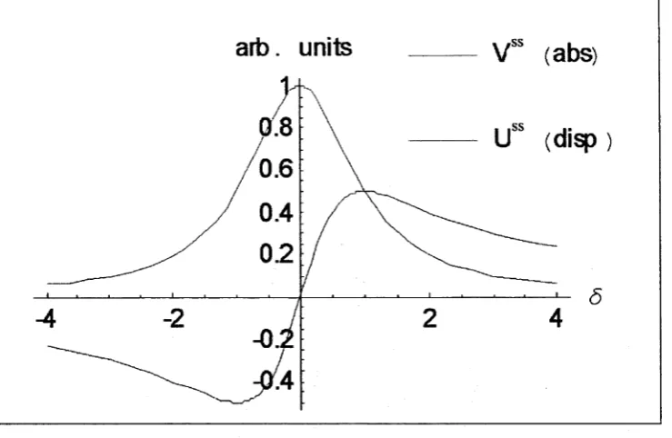
This new description of the Bloch equations allows for physical interpretation of these spher ical coordinates. W is the population difference, U is the dispersion and V is the absorption. The steady state solutions for eq. 1.13 is given by

Uss

y s s

w ss

We1XJ x*

D w e* 1Xxr

D

{gj

+ r 2)

D

where

(1.14)

D = 1 (T2 + 8 l ) + T Xl

(25)

arb. units

Figure 1-6: The steady state solutions for the driven TLA. The absorption is given in red, the dispersion in blue.

u \

( - r - s x

o

^

u \

f 0 1

V

=

fix

- r -Xx

V +

0

(1.15)

\ w /

\

0

Xx

~7 j

V w /

^ 7Wcq

J

Ignoring the relaxation terms for the point of demonstration and defining the Bloch vector

m = [U,V,W] then eq.1.15 is equivalent to

where

ft = [xx,o,<y

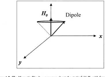
[image:25.531.85.455.64.305.2]

(26)

Figure 1-7: The Magnetic Dipole fi precesses about the static field Hq with frequency given by

the Larmor frequency coq

-H o;

= ~lmV X H0

The connection between the entirely classical case of the magnetic dipole and the semiclassical driven TLA is then clear. In the classical case, the magnetic dipole precesses about the

7 r as shown

static magnetic field with a frequency given by the Larmor frequency ujq

in fig 1-7.

[image:26.531.85.451.62.329.2]

(27)

Figure 1-8: The precession of the Bloch vector m about the vector $1, with the frequency of the precession equal to the generalised Rabi frequency.

the generalised Rabi frequency. Intuitively, it can be seen th a t the phenomenological damping terms will tend to damp the vector until it lies along the population axis, with a length given by the equilibrium population difference, W eq.

Shortly the Bloch vector model will be used to demonstrate very effectively the existence of a new transition, the Rabi transition, the study of which forms the basis for this work.

1 .4 .5 S e m ic la ssica l D r e sse d S t a te B a sis

In a manner completely analogous to the fully quantum mechanical dressed state basis, it is possible to define a semiclassical dressed state basis th a t will solve the Bloch equations (eq 1.12). It is employable in the circumstance where T = 7, i.e. the transverse and population

relaxation rates are the same. Note that for purely radiative dampening T = 2 7. The case of more general dampening is considered in section 3.5.3. To see this, define the semiclassical

[image:27.531.102.486.60.336.2]

(28)

|1) = cos6 \g) — sin# |e)

|2) = sin# |g)-|-cos# |e)

with the definitions

cos 26 — sin 26 = ~

\Lx ^“X

These states are the semiclassical analogs to the quantum mechanical dressed states em ployed earlier. Under this transformation, the Bloch equation becomes (with T = 7)

# 1 2 — i t t x p i 2 — T ( p12 — P12)

Wd = - T ( W d - W ? )

where

# 2 2 ~ P u

y

r

weq

1

^ — ---= —~ r W eqsin 26

A o L x Aj

c

~ ^ W eq = W eq cos 26

\ lx

Here, p12 refers to the coherence in the dressed state basis, and Wd refers to the population difference between the dressed state basis states. The transformed Bloch equations are easily solved, giving for the steady state solutions

Wd =

P12 =

W ? =

p& = P l l L ( - n )

(29)

Here, the Lorentzian function L (ck) is defined, and will be used extensively throughout this thesis.

L ( a ) = La (ck) ~ i L D (a)

with the absorptive {La) and dispersive (Lp) Lorentzians

La

(ck)

Ld

(a)

r

r2 + ck2

Ck

r2 + a2

These steady state limits then give the steady state solutions for the dressed states. In the original basis (bare state basis), the results become

psgse = cos2 0p\2 — sin2 0p2i -I- cos 6 sin 0W$S

W ss = (cos2 6 — sin2 6) W$s — 2 cos 0 sin 0{p\2 + P2 1)

1.4.6 Geometrical Interpretation of the Dressed States

As has been seen, the Optical Bloch equations leads to a simple geometrical interpretation, completely analogous to the fully classical magnetic dipole. Recall the basic dynamics of the TLA as being represented by the vector equations

— m = —m x il dt

This can be extended to include homogeneous damping terms

(30)

m eq = [0, 0, W e g ]

The dressed state basis is then simply a rotation th at aligns the transformed z' axis with

Q , simplifying the system. In this basis, the Bloch vector ttV precesses about the z ' axis, relaxing to the steady state ra ' = [— sin 29,0, cos 26] Weq.

1 .4 .7 T h e M o llo w S p e c tr u m

The semiclassical dressed state basis is used extensively throughout this thesis and so to intro duce its use, a calculation of the standard Mollow spectrum can be performed [3]. This sort of calculation will be used frequently, and so it is useful to see it used in a simple circumstance. In the Mollow spectrum, a strong pump field is applied to the TLA, and then a weak probe field (frequency cup and small Rabi frequency u) is scanned across the transition, and its absorption measured. The equations of motion that describe this are given by

where the probe field detuning 6p = ujp—cjx. The solutions can be written as a power series in the weak parameter a

The zeroth order equations are simply Eq. 1.12, and have been solved above, to give

2

ix(Peg - Pge)

+

2ia

(

h ge

-

« '<M) —

T (W —

W ‘1)

i^X-W — i —We i6pt

2 2

w =

i r (0) +

aW ^

+ q2IT(2) + ...

(31)

i®

= ( « « - r

)p$-i^ww

w m = 2i\(p™ - p£>) + 2 i(p g ^ M - pg> e-i4' ‘) - r iv « 1)

To proceed, transform these equations into the dressed state basis

p[lJ = (•iÜx- T) p™ + sin 20 (e ^ * + ^ (cos2 dei6^ - sin2 0e_ i w j 0)

wj1} = -n rd(1) + i

(cos2 0 e ^ ‘ - sin2 e- ^ * ) p ^ - i (cos2 0e“ i5pf - sin2 0 e ^ ) p j?

which is easily solved by substituting in the zeroth order solutions. After putting in the zeroth order solutions, the solutions to the first order in the probe beam power become

P n = P+eiM + P - e - “ "1

l i f 1 = W + ei4»‘ +

where

p+ = ^ sin2 26>nre9L ( - f i x) + cos2 0 cos 20tTe<^ L (<5P - ftx)

p_ = - i ~

Q

sin2 2 0 rW e<7L ( - f i x) - sin2 0 cos 20VTe<^ L (-<5P - fix) W+ = - i f a sin 2GTWeq (cos2 0L (ftx) + sin2 OL ( - f i x)) L (<$p)

W~ = U a s \ n 2 G Y W eq (cos2 GL {- Yt x) + sin2 0L (Qx)) L (~ 6 P)

(32)

Pge (Ö p) — COs2 9 p + ~ » ill2 + 7y s in 2Ö

= - i | cos2 9 Q sin2 26>rWe<?L ( - f t x) + cos2 6> cos 29Weq^j L (6P - Qx)

sin2 0 Q sin2 26TWe<7L ( Q x ) - sin2 9 cos 26>We<7j L (<5p + flx)

- i f a s i n 2 29TWeq (cos2 0L (Qx) + sin2 9L ( - Q x)) L (6P )

The familiar solution is then a series of three Lorentzians at 6P = 0,±f2x, each having a weight summarised in the following table

L o r e n tz ia n W e ig h t

L ( s p - n x) — cos2 9 (cos2 9W^q — sin 29pcq2L (—f ix))

L (bp + fix) i \ sin2 9 (sin2 9W^q + sin 29peq2L (12x))

L(6„) ^i sin 29peq2 (cos2 9L (Qx) + sin2 9L (—fix))

Notice that the sidebands (Sp = dzfix) have a weight th at is broken up into two parts. The first part is proportional to the equilibrium population difference in the dressed states, W^q,

and the second part is due to a contribution from the steady state coherence that is set up by the driving field p^q. As well there is a component at 6p = 0 that is proportional to the coherence.

In the limit of well separated peaks, i.e. Qx T, it is possible to make the following simplification

Lf f l x) ~ - i L D (Qx)

and since Ld (fix) 1/^x? if can be noted that when the pump field is off resonance

I

Ld

(^x)|<|W

de<7

(33)

L o ren tz ia n W eight

L ( 6 p - n x) —i \ cos4 6 W ^ q

L (6p+ l^x) i

|

sin4 9 W ^ q

L( »p) ^ sin 26 p \ q2cos 2 6 Ld{Ltx )

The actual absorption and dispersion spectra are given by

A{ 6 P) = -% pge (Sp)

= i cos4 8 W ? L A (Sp- fix) - ^ sin4 9 W ? L A + fix) + ^ sin ‘10py> cos 20L i, (Qx) Lit (<5P)

D( SP) = UPge(6p)

= cos4 0 W ‘'‘Ld (Sp - Slx) + t sin4 S W ^ Ld («, + flx)

— ^ sin ^0pW c°s 20 Lu (Llx) Lu (bv)

This is the familiar off-resonance Mollow spectrum (in the high power limit). Three peaks are evident. The two oppositely signed peaks La (ßv — Ltx) and La (ßv + Hx) are due to tran sitions between the dressed states, just as in the fully quantum mechanical case. The third peak, much smaller since it is proportional to Lq (Llx ), is a dispersive shaped peak centered at

6p = 0. This peak is due to the steady state coherence that arises in the driven system peq2.

The on-resonance (Sx = 0) case leads to the result (to the same approximation as above)

L o ren tz ia n W eig h t

L( s p - n z ) \t w * l d(nx)

L (Sp4* f2x) - ± r w ei<LD (nx)

- \ i V W ‘qL A (fix)

(34)

1.5 T he R abi Transition

The TLA uses only the transverse dipole moment as the light-matter interaction. In this case, the incident radiation is polarised at right angles to the axis of the TLA and the population cycles between the ground and excited states at a rate given by the generalised Rabi frequency. A natural extension of this is to then study the effects of applying more strong fields and to study the effects of this on the dressed state formalism. While this has been studied extensively theoretically [17]-[31], there is a paucity of experimental results [32]-[38],[45]-[46],[47]-[50]. Ficek

and Freedhoff [51] have also written an excellent review article that sums up much of the work

to date. Most of these studies centre on the idea of using another x polarised field as the second driving field. In this thesis, a different scenario will be examined, that of driving the driven TLA with a z polarised field.

It has been shown theoretically [56]-[58],[39]-[42]and experimentally [43]-[44] th a t if a field polarised in parallel with the population axes is applied, then a resonance at the generalised Rabi frequency can be seen. To see this, modify the “light+m atter” interaction to include a

permanent dipole moment. This allows the TLA to couple with z polarised fields. To see how

this will generate the Rabi transition, consider the geometrical model shown above.

Previously, a single x polarised field (call it Fieldx) is coupled to the transition via the stan dard (see Fig l-9a) transverse dipole moment interaction. Now add an additional z polarised field (F ields, coupled to the transition via the permanent dipole moment (the theoretical de tails will be expanded later). Go to the rotating frame, as before, and discard the anti-resonant term (the RWA). Note that since the rotation is around the z axis, Fieldz is unaffected. Fig l-9b shows the picture as it stands.

Recall then th at the dressed states basis transformation rotates the axis so th a t it is in line with fb Once this is done, note that there are now two components to Field2 in this frame. One is perpendicular to the new z' axis, and the other is parallel. The field perpendicular to the z' will then drive the transition which is characterised by the vector Q , in exactly the same way that the original Fieldx drove the transition characterised by the original transition frequency

(35)

t Field — —

o, —

Ira n s form to the Dressed State basis

B a sic TLA

Transform to Rotating Frame in the Dressed State Basis

0, —

Transform to the Rotating Frame and add z Field

Figure 1-9: The four stages towards understanding the Rabi transition. In (A), the standard TLA is presented, with an on-resonance x polarised field (Rabi frequency \ x ) interacting with

the bare transition of frequency u>q. (B) sees the system transformed to the rotating frame

[image:35.531.54.484.143.455.2]

(36)

the study of this transition that forms the bulk of the work of this thesis. Fig l-9c shows this transition geometrically in the case where Field* is resonant.

The second component of Fields in this basis, the one parallel to SI, is part of a higher order process which will be studied in more detail later. Actually, at this point, it is plain in what direction the theoretical analysis should proceed. There is now, in this new basis, a system which is completely analogous to the original system, where Field* was driving the original transition. Clearly, then, a similar set of transformations (rotating frame, RWA, dressed state basis) can be applied to shed insight into this system, which is in fact performed in Chapters 2,3.

The Rabi transition behaves in a similar fashion to the normal TLA, allowing for many of the same analysis techniques to be applied. In fact, the Rabi transition can be driven by a strong pump field, and then examined using a probe beam th at studies either the original transition itself, or the Rabi transition. The details of this will be covered in a later chapter. Again, this system is theoretically accessible to relatively simple analysis, which employs the

Doubly Dressed States, a natural extension of the dressed state analysis.

The doubly dressed states formalism is not a new concept, and has been used recently to study interactions of TLAs with polychromatic radiation [51]. The formalism has been used to successfully study the case of two Field*’s interacting with a TLA (much of it since 1998, when this work was performed), however the complexity of the interactions mean th at in general the solution is perturbative in nature though there are special circumstances where a more accurate solution is gained. However, what makes the calculation in this thesis different is the orthogonal nature of the interacting fields, Field* and Fieldz. As will be seen, this naturally lends itself to an elegant symmetry in the dynamics, where Field* and Fields interact in entirely distinct regimes. This enables the doubly dressed states to be used very naturally and accurately, and they remain a good form of analysis for a broad range of experimental parameters. It will also be shown that the extension of the work to include the concept of triply, quadruply and so on dressed states is equally intuitive and natural. To appreciate this, it will be worthwhile to carefully present the calculations in their entirety.

(37)

driven system. Chapter 3 also refines the theory somewhat, using numerical techniques to calculate higher order terms, the Bloch Siegert shift associated with the Rabi transition and so forth. The experimental results (the experimental system is introduced in Chapter 1) are then compared with the theoretical results in Chapter 4.

The Rabi transition is then studied by applying a z polarised field to the driven system. To examine this transition, first assume that the z field is weak. T hat is, the TLA is strongly driven with a Fieldx and then probe the system with a weak Field2. So the system is coupled to one classical x polarised field,

E x — x E x cos a)xt

and one z polarised probe field

E z = z E z cos u zt

The Fieldz is coupled to the TLA by the permanent dipole moment, with Hamiltonian

H - /x • ^ E x + E z^j

cos U)xt + h 0 0

0 2Xz

cos u zt

where the semiclassical Rabi frequencies are defined by

ß x . E x

h

ß z ^ z

h

(38)

(in the rotating frame) become

J t Pge = { * ( 6 r + 2 x * C O S W * t ) - r } p 9 e - i ~ W

W = iXz (Peg ~ ~Pge) ~ T ( W - W ‘<)

To examine the Rabi transition using a probe beam, assume th at \ z is small. The solutions are then written as a power series expansion in \z->

e-g-Pge Pge "T X z P g e T X z P g e T

The steady state zero order terms have already been calculated above, and expressed in the semiclassical dressed state basis they become

Pi? = p\ Il ( - qx )

ww = wedq

Writing out the first order equation, the first order term equations of motion are obtained

P (ge = ( i S x - n + 2% cos «>* - % y *>

= iXx ( p § ~ P{g f)

These are then converted to the semiclassical dressed state basis as above

Pl2

—

(*^x

- r)

p ^2 + 2i x " COS L ü z t p ^ ~ W z COS UJz t W ^

(39)

x'z = - s i n 2 0Xz = - ^ i X z

X" = cos 2 9Xz = ^ - X z

Then these can be easily solved for the first order solutions

= a ^ ' + a - V " * *

= c1e*“’’t + c r'e- “ ' 1 The coefficients then become

a1 = ^ fa z P i2 ~ ’X ' z ^ ) L (u z - Qx)

= ^cos26>sin26>x2W e9(l - T L ( - Q X)) L ( u z - Qx)

a ' 1 = ^cos26>sin26>x2V^e9( l - r L ( - Q x) ) L ( - a ; 2 - Q x)

c1 = - r s m 2 20x z WeqL D ( n x) L { t j z)

c - 1 = - T s in 2 20XzW eqL D (t yx)L{-u;z)

These results are transformed back into the bare state basis (for the population)

W — — sin 26 (pl2 + p2i) + cos 2OWd

= W° + W l eiu’zt + W ~ l e~iu,zt

(40)

W l = — sin 26a} — sin 20 (a u ) 4- cos 20c1

=

k L

((1

- VL ( - f i x)) L

(a>* - n x) + (1 - r

L{ Qx) ) L ( u z +

n x) ) ~

T Ld (Qx) L

(

w

2)J

where

k = cos 20 sin2 20xzPEe<7

Examining the high power limit (i.e. Qx T), it is possible to simplify

L{ ÜX) = L A (Qx) - i L D (Qx)

by noting th a t Lq (Ttx) L A (f2x); hence

L ( Q x) ~ - i L D (Qx)

and so

T Ld ( ß * ) < 1

leading finally to the equations

w 1 = <4

(lu z ( - q x

(w2 + n*))

This obviously shows a resonance at the Rabi frequency. Looking at that component in particular, the absorption and dispersion are calculated:

abs = S W 1 = ^ L A (u>z - Ü x)

(41)

The weight of the probe absorption spectrum at the Rabi frequency is then given by

^ ^ cos 20 sin2 20xzW eq

= \ sin2 W XzW f

The spectrum of the probe beam then shows a clear signal at the Rabi frequency, showing th at the Field* does indeed interact strongly with the permanent dipole moment. Notice that the line’s weight is proportional to the dressed state population difference. This means that there will be no signal (to the lowest order) with an on resonance Field* (6X = 0). This is in line with intuition, since the on-resonance case will equilibrate the dressed state populations, quenching any net absorption in the final results. Note th at the maximum signal size will be when Sx = Xx-> balancing the strength of the interaction of the probe beam with the dressed states, sin 29 \ z with the resultant population difference W^q. Also, because the size of the Rabi transition is proportional to W j9, in the case where 6X < 0 (i.e. when the driving field is on the high side of the transition), W%q > 0 and so the transition is emissive. On the other hand, when 6X > 0 , the Rabi transition is absorptive.

The motivation then of this thesis is to examine this new transition. Previously, the transition was recognized, but only used to measure the Rabi frequency in NMR experiments, using the transition as shown above [56]-[58]. This thesis intends to take this analysis further, and study the implications of treating this transition as a whole new TLA system in its own right. This new TLA has several advantages, including tunable characteristics (transition size, dipole moment etc.). Also, inhomogeneous broadening is considerably dampened in the transition. To see this, note that resonantly driving a inhomogeneously broadened line (linewidth A) will produce an ‘average’ Rabi transition of (assuming the high power case where X » A)

(42)

so the approximate inhomogeneous broadening of the new line is

~ 2

(x) A

The Rabi transition will then provide perhaps a “more perfect” TLA th at can be examined. Also, as will be seen, the dynamics of a doubly driven system can be examined in a theoretically tractable manner, leading to an intuitive generalisation of the dressed states, the so called doubly dressed states. This idea can even be expanded to the higher orders to include triply dressed, quadruply dressed and so on states. These higher order interactions provide a plethora of new interactions, both in the regime of the original transition, and in the regime of the Rabi transition. Chapters 2,3 will examine the theoretical basis of this transition, as well as the results for the driven Rabi transition. Chapter 4 will then present the experimental results and compare them to theory.

1 .6

T h e E x p e r im e n ta l S y s te m

To understand the experiment, it is necessary to understand two distinct areas - the N-V centre (Nitrogen Vacancy centre) in diamond (the system that will be examined) and the Raman Heterodyne technique (the detection method). The N-V centre in diamond provides a convenient system to study, where impurities in the diamond allow the examination of a system th at very closely approximates the TLA. This TLA can be excited with radio-frequency (RF) fields (both x polarised and z polarised) and probed with another, weak, RF field. The detection method used to examine the spectrum is the well known Raman Heterodyne method, where optical frequencies ‘beat’ with the applied RF fields to present the final spectrum for analysis.

1 .6 .1 N -V C e n tr e in D ia m o n d

(43)

has a single electron associated with it, while the broken bond with nitrogen has two floating electrons. Thus, five electrons are involved. It is well known, however [64]-[71] that the orbital ground state (the 3 A state) is a spin triplet so it would seem there is an even number of electrons

involved. This was generally explained by assuming that the centre will trap another electron. There has been some controversy over this theory [73]-[75], however, what is known is th at ESR (Electron Spin Resonance) studies of the ground state NV-Centre demonstrate a spin triplet system, two levels of which form the main TLA examined in this thesis.

Also, due to the symmetry of the system, there are in fact four equivalent orientations (axes of symmetry) for the N-V Centre. The centre has trigonal symmetry of point group C3,, where

the C3 principle axis lies along the N-V axis. When a static magnetic field is applied along one of the symmetry axes, the other three centres are magnetically equivalent and this aligned symmetry axis of the N-V centre is then considered to make up the nearly-ideal TLA which is examined in this thesis. This TLA then occurs at RF frequencies, and only the observation of the centre needs to be examined.

The N-V Centre also exhibits optical, as well as RF, resonances. The centre can be excited with optical frequencies, where the first excited state is centered at ~ 638 nm, and measurements [76]-[78] demonstrate that the ground and excited states are describable in the representation A and E respectively. The 3A to 3E transition is the key (optical) transition that is exploited

as the detection method for this thesis - the Ram an Heterodyne detection technique. The 3E

transition has a lifetime of 13 ns [79] and an inhomogeneous linewidth of ~ 800 GHz (the large broadening is due to large variations in crystal strain).

To summarise to date, the NV centre’s ground state is a spin one system, which is used to generate a TLA which is accessible at RF frequencies, and the transitions are observed using the optical transition with the excited state of the N-V centre. Examining the ground state sublevels in more detail, the 3A state is split by crystal field interactions into a singlet state (ms = 0) and a degenerate doublet (m s = ±1) separated by 2.88 GHz. If a static magnetic field is applied along the N-V centre axis, it lifts the degeneracy between the m s = ±1 sublevels.

As the power is increased, the m s = —1 approaches the m s = 0 state. As they approach each

(44)

m=+l >

m =-l>

Anticrossing region

where the wavefiinctions are highly mixed

m =0>

1028 G

Figure 1-10: The basic energy level scheme associated with the N-V Centre 3 A ground state. The state field Ho is applied along the symmetry axis which causes mixing between the levels at the anti-crossing region.

high level of mixing between the levels, which greatly enhances the level of interaction available to the system. The mixtures of the states lead to two quantum wavefunctions if>_1 and ipQ which are mixtures of the spin states |0 ) , | — 1)

\1 > o ) = a|0) + 6 | - l )

| ^ - i ) = — a | —1) + ft |0)

[image:44.531.167.425.56.347.2]

(45)

The situation is complicated somewhat by the nuclear spin hyperfine levels in the \ms = — 1) and Im s = 0) states, shown in fig 1-11. One of the areas that needs to be examined is the complication due to the extra levels that are associated with the TLA (in effect 3 sublevels). Transitions between the hyperfine levels between the wavefunctions above form the so called EPR (Electronic Paramagnetic Resonance) transitions, and between the nuclear spin substates within each wavefunction form the TLA called the NMR subsystem. Hence, the system ex amined actually consists of two regimes, the EPR (~70 MHz transition) and the NMR regime (~5 MHz). The bulk of the data taken in this thesis is taken in the EPR regime, in which higher Rabi frequencies are obtainable making it possible to observe the transition which is the object of this study. The EPR transition studied then has hyperfine structure associated with the following significant transitions (with their relative energies)

|0,0) « 1-1,0) E = 0.0 M H z

I0.-1)

<- 1 -1 ,-1 ) E = 2.4 M H z

10,1} - 1-1,1) E = -1 .8 M H z

(46)

0.0 —

\ f

---10,0>

in w ™s=0

- - 1 1 0 ' ' 0 . 0 ““

111'' 1

J

-7.0 —

1 1» 1 Ills---1 ---1-1,-1>

EPR transitions ~ 70 Mhz

NM R transitions ~ 5 MHz

Figure 1-11: The energy level scheme for the experimental system. EPR transitions are between the ms = 0 and the ms = — 1 electron spin states. Each of these states is a further nuclear spin triplet, and this hyperfine structure is shown here, with the energy levels separating them. This gives rise to two experimental regimes, the EPR and NMR regime (shown in colour code).

1 .6 .2 R a m a n H e te r o d y n e D e te c tio n

The Raman Heterodyne Detection technique is a very sensitive detection technique that allows the experimenter to directly access the absorption and dispersion spectra for a system (in this case the NV - Centre driven by RF fields). It relies on the coherence of the system that is produced by the RF fields, and then optical frequency detection methods are used to observe the coherence (in both the cw and transient regimes). It is a well known detection method [61], and nothing will be added to the literature by a lengthy exposition here, so only a brief introduction will be presented here.

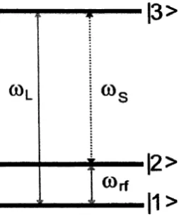
The technique was first reported by Mlynek et al. [80], and has since been used for detecting NMR (Nuclear Magnetic Resonance) and EPR (Electron Paramagnetic Resonance). Raman Heterodyne detection, as mentioned, does not give the populations of the levels, but instead allows direct observation of the coherences. Referring to Fig 1-12, the Raman Heterodyne technique is used in the case where the RF transition in question is coupled to a third level via the optical frequency laser (frequency u>l) while being driven coherently by a RF field (frequency u)rf).

[image:46.531.221.405.73.259.2]

(47)

|

3 >

|

2 >

H>

Figure 1-12: The energy level scheme for the Raman Heterodyne detection scheme. An RF field excites the |1) |2) transition (the experimentally interesting one) and a laser excites the jl) |3) transition.

in coherence between levels |2) |3) which produces a Stokes Raman signal E s at frequency

ljs = ^3 2- This stimulated Raman signal beats w ith the incident laser frequency to produce a beat frequency of cjrf, and it is this beat signal which is detected by a photodiode. For the particular case of the N -V Centre, the N M R and EPR centres are both magnetically allowed

(the |1) «-> |2) transition) and transitions between the hyperfine levels of the 3A and SE states provide the optical transitions th a t are allowed, to enable the Raman Heterodyne procedure to

be used [82].

It has been shown previously [81] that the resultant intensity of the beat signal I s for optically thin samples is given by

I s a (Re (p2i) cos cur f t + Im (p2i) sin a>rft)

where the angular brackets around the p2i denote an average over optical and RF inhomo

geneities. Note the coherences here are the slowly varying parts w ith respect to ujrf. Clearly, the intensity of the signal is made of an in-phase and an out-of-phase component. These can

[image:47.531.201.328.66.223.2]

(48)

1 .6 .3 E x p e r im e n ta l C o n fig u r a tio n

The experimental schematic is shown in Fig 1-13. The N-V Centre was provided by a sample diamond crystal measuring approximately 1 mm3. The sample was mounted in a pair of RF coils (made in house) th at were mounted at right angles to each other. The coils and sample were then mounted in an Oxford Instruments 3T helium exchange gas cryostat (including a superconducting magnet). The superconducting magnet provided the static magnetic field to lift the degeneracy of the spin ±1 states (see Fig 1-10). The sample was mounted in such a way th at it could be rotated with respect to the applied magnetic field, allowing the experimenter to achieve an optimum signal strength by aligning the crystal’s [111] direction.

The Raman Heterodyne detection technique employs an optical probe with a wavelength of around 638 nm (the colour transition in the N-V Centre). The probe is produced by a coherent CR599-21 cw single mode dye laser (power ~few mW), which was pumped by a Spectra Physics Stabilite 2016 cw Argon Ion laser (power ~4W ). The probe beam was focused on the N-V Centre sample, and the output Raman beat signal was detected on a New Focus 1801 DC-125 MHz photodiode.

The RF fields were then applied to either of the two coils. One coil would generate any x polarised fields, the other z polarised fields. These fields were generated by various RF power supplies with powers ranging from -70 dBm to T2dBm. So, in the instance most used in this experiment, there would be an x polarised pump field at the EPR transition, a z polarised pump field at the Rabi transition, and a weak x or z polarised probe field, resulting in three RF power supplies. The probe field power supply originated from the spectrum analyser, the Hewlett Packard 4396A Network/Spectrum Analyser. The signals were summed and then passed through the coils, before being dumped onto a 50 D load.

(49)

Light path

Coil z

Superconducting / Magnet

Diamond Sample

Coil X

r.f power amplifier Various r.f power

supplies

Various r.f power supplies

Photodiode Dye Laser

Argon Ion Laser

HP 4396A Spectrum Analyzer

(50)

solve for the dynamics of the Rabi transition.

1 .7

S u m m a r y

(51)

A study of the transition at the Rabi frequency in the driven two level atom