Circular local likelihood

https://doi.org/10.1007/s11749-017-0576-9

O R I G I NA L PA P E R

Circular local likelihood

Marco Di Marzio1 · Stefania Fensore1 · Agnese Panzera2 · Charles C. Taylor3

Received: 5 June 2017 / Accepted: 20 December 2017 / Published online: 21 January 2018 © The Author(s) 2018. This article is an open access publication

Abstract We introduce a class of local likelihood circular density estimators, which includes the kernel density estimator as a special case. The idea lies in optimizing a spatially weighted version of the log-likelihood function, where the logarithm of the density is locally approximated by a periodic polynomial. The use of von Mises density functions as weights reduces the computational burden. Also, we propose closed-form estimators which could closed-form the basis of counterparts in the multidimensional Euclidean setting. Simulation results and a real data case study are used to evaluate the performance and illustrate the results.

Keywords Bessel functions·Circular data·Density estimation·Log-likelihood· Numerical integration·Product kernels·von Mises density

Mathematics Subject Classification 62G07

B

1 Introduction

A circular observation can be represented by a point on the unit circle and measured by an angleθ∈ [−π, π), after both an origin and an orientation have been chosen. Its real-line representation is provided by the equivalence class{2mπ+θ,m∈Z}, and therefore standard linear methods are not suitable for circular data analysis.

Classic examples include flight direction of birds, wind and ocean current direction. Time of day, or time of year are also obvious candidates for directional modelling. When, along with a direction, we report also the time of the day when it has been recorded, we are collecting two-dimensional circular data. In zoology many multi-dimensional instances arise. For example, Fisher (1993) considers the orientations of the nests of noisy scrub birds along the bank of a creek bed, together with the corresponding directions of creek flow at the nearest point to the nest: here the joint behaviour of these random variables is of interest. Multidimensional circular data are also commonly found in the analysis of protein structure (Lovell et al.2003). In political science, Gill and Hangartner (2010) study directional party preferences in a two-dimensional ideological space for the German Bundestag elections.

Maximum likelihood estimation is a common approach in many statistical prob-lems, although it requires an assumption that the unknown target belongs to a restricted class of functions. To obtain more general models, Tibshirani and Hastie (1987) intro-duced the concept oflocal likelihood. They proposed to fit a regression function using only the observations falling within a certain window around the estimation point. In the context of density estimation, local likelihood requires spatially weighting the log-densities. Depending on the smoothing degree, the methodology can be viewed, in practice, as basically parametric or nonparametric.

The log-densities can be modelled in various ways corresponding to various techniques. Hjort and Jones (1996) have established a general framework, where a parametric family is locally modelled, by allowing its parameters change along the sup-port. Loader (1996a) focused on the use of log-polynomials. Eguchi and Copas (1998) proposed an alternative construction and focus on properties related to asymptotics when the smoothing degree is fixed. Delicado (2006) proposed a unified formulation of these local likelihood approaches based on the concept of sample truncation.

non-Euclidean data. However, small bias estimation in nonparametric circularregression

has been introduced by Di Marzio et al. (2009, 2013).

Recently Di Marzio et al. (2016) have presented a computational study where den-sity estimation based on local polynomial likelihood is investigated for two practical issues not treated in this paper: the impact of the density normalization step when the sample size is moderate; and the effectiveness in identifying the number of population modes.

In Sect. 2 we present the model together with some major features of the esti-mators, while Sect. 3 is devoted to asymptotic accuracy. In Sect. 4 we show how some numerical aspects can be greatly simplified if the d-fold product (d ≥ 1) of von Mises densities is used as the weight function. After some asymptotic approximations and interpretations, two new estimators are proposed, which could inspire similar counterparts in the multidimensional Euclidean set-ting. Section 5 is devoted to numerical experiments where the main theoretical properties are confirmed in small to moderate sample sizes. Finally, Sect. 6

contains a real data example related to the three-dimensional structure of pro-teins.

2 The model

Let f be a circular population density, i.e. a non-negative, 2π-periodic function with

[−π,π)d f =1,d ≥ 1. We want to estimate f atθ ∈ [−π, π)d, using a realization

θ1, . . . ,θnof a random sampleΘ1, . . . ,Θndrawn from f.

Once the domain of f has been partitioned into S equal cells, sayC1, . . . ,CS,

letns andPs denote the cell counts and probabilities, respectively. Due to the mean

value theorem we can write Ps = f(θs)(2π)d/S for someθs ∈ Cs. The likelihood

iscS_s=1Pns

s subject toSs=1Ps =1, wherecis a multinomial coefficient. Using

Lagrange multipliers, this leads to a penalized log-likelihood

L(f)=logc+

S

s=1

{nslogPs −n Ps}.

Assuming that the number of cells is sufficiently large so that not more that one observation falls in each one, the sum can be taken over then observations,ns =

1, and Ps can be replaced by Pi, the probability for the cell containing the ith

observation.

Forβ ∈ [−π, π)dwith jth entry denoted byβ(j), we define the kernelfunction

K_κ1,...,κd(β) = d

j=1Kκj

β(j)

, where K_κj is a circular kernel with zero mean direction and concentration parameterκj ≥ 0; see Definition 1 given by Di Marzio

et al. (2011). The weight function K_κj is usually chosen to be a continuous density function whose support is the circle with the property that asκj → ∞the density

tends to concentrate at the mode. If we spatially weight each summand ofL(f)by

Lθ(f)=

n

i₌1

K_κ1,...,κd(θi−θ)log f(θi)−n

[−π,π)d

K_κ1,...,κd(α−θ)f(α)dα.

The number of observations contributing to the estimate in the jth direction is related to the magnitude of the concentrationκj.

The main motivation for defining an estimator of f(θ)as the maximizer ofL_θ(f)

over f lies in the property Ef[L_θ(f)] ≥Ef[L_θ(g)]for all non-negative functionsg,

with equality holding when f(u)=g(u), for any u ∈ [−π, π)d. This is shown by noting thatx ≥ logx+1 ifx >0. The conditionx >0 extends our methodology also to non-negative regression function estimation.

As a model for log f consider a (2π-periodic)pth degree sin-polynomial (Di Marzio et al.2009)

Pp(λ)=a0+

p

s₌1

(S_λ)⊗sas

s! ,

withλ ∈Rd,a0 ∈ R,as ∈Rd

s

,s ∈(1, . . . ,p),S_λ = sin λ(1), . . . ,sin λ(d),

andS⊗_λsdenoting thesth order Kronecker power ofS_λ. We callPpasin-polynomial

because the functions sinsare reminiscent of the monomial bases for ordinary polyno-mials. Likewise, we associate the termslinearandquadratic, respectively, toP1and

P2. We use sin functions since the absolute value of the sine of a difference depends

only on the magnitude of the smallest arc between the two respective points. The use of a simple difference, as for standard local polynomial modelling, would not be suited to angles because it depends on whether the origin belongs to above the smallest arc or not. In both cases, the sign depends on the orientation choice, that is also arbitrary, but this is not relevant due to the symmetry of our weight functions.

Since f is determined bya=(a0,a1, . . . ,ap), we get

Lθ(a)= n

i=1

K_κ1,...,κd(θi −θ)Pp(θi −θ)

−n

[−π,π)d

K_κ1,...,κd(α−θ)exp(Pp(α−θ))dα.

DifferentiatingL_θ(a)with respect to the elements ofa, and setting these partial derivatives equal to0, leads to_sp₌₀dsequations:

1

n

n

i=1

A(θi−θ)Kκ1,...,κd(θi−θ)

=

[−π,π)d

A(α−θ)K_κ1,...,κd(α−θ)exp Pp(α−θ)

dα, (1)

whereA(λ)=vec

1,S_λ, . . . , S_λ⊗p/p!

θ

density estimate

0 1 2 3 4 5 6 0 1 2 3 4 5 6

0.05

0.10

0.15

0.20

0.25

0.30

0.35

0.0

0

.2

0.4

0

.6

0.8

θ

density estimate

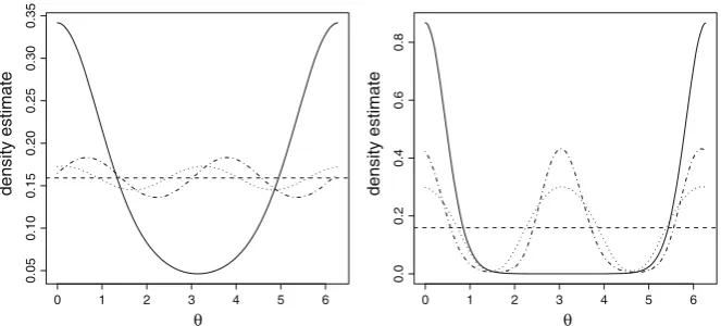
Fig. 1 (Normalized) density estimates for samples of size 100 from a von Mises distribution with concen-tration parameter 1 (left) and 5 (right), forP0(dashed),P1(dotted), andP2, (dash-dot) with smoothing parameterκ=0. True density is continuous line

If log f is smooth enough atθ, the sin-polynomialPprepresents a series expansion

of log f up to orderp, and solving the system of Eq. (1) foragives the estimatesaˆ=

(aˆ0,aˆ1, . . . ,aˆp)ofa˜ =(a˜0,a˜1, . . . ,a˜p), where, forθ ∈ [−π, π)d,a˜0=log f(θ)

anda˜s is the vector of the mixed partial derivatives of total ordersof log f atθ. For

example,a˜1is the gradient vector, anda˜2 =vec(H), whereHdenotes the Hessian

matrix. Arguments in Loader (1996a) assure the existence and uniqueness ofaˆsince cartesian products of circles are compact. Setting g = log f, andgˆ(θ) = ˆa0 the

density estimate atθ∈ [−π, π)dis then given by

ˆ

f(θ)= exp(gˆ(θ)) [−π,π)d exp(gˆ(θ))dθ

. (2)

When p =0, formula (2) simplifies to the standard kernel estimator (Di Marzio et al.2011), whereas forp>0 it generally becomes nonlinear and the denominator is required to make it abona fidedensity. It isrotationally invariant, that isaˆ = ˆa∗, where

ˆ

a∗is the estimate using translated dataθ1+ω,θ2+ω, . . . ,θn+ω,ω∈ [−π, π)d.

Thus, if we rotate the initial direction byωthe estimate is not affected. This, in circular statistics, is an important property as the choice of the origin is arbitrary.

3 Accuracy

As a starting point, we establish that asymptotic properties of estimator (2) can be conveniently expressed by referring to those of the estimators of log-densities. This can be seen by a very general argument that requires consistency of the estimator and smoothness of both the population and the estimate. To simplify notation, we initially consider the one-dimensional case.

Using againg =log f, in virtue of Corollary1, we have that, for largen, Rn =

ˆ

g−g≈0 and so exp(g+Rn)≈ f×(1+Rn). This shows that the rate of convergence

of the log-density estimator atθ ∈ [−π, π)does not change when we exponentiate it, whereas its magnitude varies due to the multiplicative factor f(θ). Clearly, this

transformation improves the estimation at the tails, and, more generally, over the regions where f(θ) <1. Such regions are generally a large part of the support when we note that our densities are continuous functions over [−π, π). Concerning the convergence rate of the normalized estimator, we see that

f ×(1+Rn)

1−

f ×Rn

= f ×(1+O(Rn)),

so the rate of convergence does not change even after normalization. Coming to the magnitude of the mean integrated squared error (MISE), it is interesting to note that above expression makes it possible to invoke Theorem 1 of Glad et al. (2003). They prove that, when the un-normalized area is bigger than one, then it does not worsen if we add to it a fixed quantity that makes its integral equal to one. This result can be considered very strong because it holds for any sample size. Obviously, if the area of our estimate is smaller than one, this theorem will not apply; however, we can still be confident that severe, often negative, bias at the peaks has been reduced. Comparisons of normalized and un-normalized estimators can be found in Di Marzio et al. (2016). In general system (1) has only numerical roots when p >0, and direct accuracy calculations are impossible, and so we expand (1) to obtain an expression for the estimation error. We consider un-normalized estimators throughout this section.

3.1 Asymptotics

The starting point for obtaining asymptotic properties is the expansion of system (1), foraˆarounda˜,

1

n

n

i=1

A(θi−θ)Kκ1,...,κd(θi−θ)

−

[−π,π)d

A(α−θ)K_κ1,...,κd(α−θ)exp

˜

Pp(α−θ)

dα

where P˜p(λ) = ˜a0 +_sp₌₁(S_λ)⊗sa˜s/s!, and J˜ =

[−π,π)dA(α − θ)A(α −

θ)_Kκ

1,...,κd(α−θ)exp

˜

Pp(α−θ)

dαis the Jacobian matrix of the local likelihood system ata= ˜a. It follows that

ˆ

a− ˜a≈ ˜J−1

1

n

n

i=1

A(θi −θ)K_κ1,...,κd(θi−θ)

−

[−π,π)d

A(α−θ)K_κ1,...,κd(α−θ)exp

˜

Pp(α−θ)

dα

⎞ ⎟

⎠. (3)

Starting from Eq. (3), asymptotic bias and variance, for the case of order p≥1 of the approximating sin-polynomial, are provided by

Theorem 1 Define as eithe(i,i)th entry of

[−π,π)d Kκ2₁,...,κ_d(α)A(α)A(α)dα, and

assume that

(a) limn→∞κj = ∞for j∈(1, . . . ,d);

(b) limn→∞n−1ei =0for i ∈(1, . . . ,

p

s=0ds).

Moreover, assume that, for odd p, all the mixed derivatives of total order p+1of the log-likelihood function exist and are continuous in[−π, π)d, and, for even p, this also holds for all the mixed derivatives of total order p+2, then, we have

(i) for odd p

E[ˆa] − ˜a≈ ˜J−1

[−π,π)d

A(α)K_κ1,...,κd(α)(Sα)⊗

p+1 a˜p+1

(p+1)!dα f(θ)

(ii) for even p>0

E[ˆa] − ˜a ≈ ˜J−1

[−π,π)d

A(α)K_κ1,...,κd(α)

f(θ)(S_α)⊗p+2 a˜p+2

(p+2)!

+S_αDf(θ)(S_α)⊗p+1 ˜ ap+1

(p+1)!

dα,

whereDf(θ)denotes the gradient of f atθ, and1is a vector of ones of length dp+1

for odd p, and dp+2for even p>0. Moreover, for both (i) and (ii)

Var[ˆa] ≈ 1

n f(θ)J˜ −1

[−π,π)d

A(α)A(α)_K2

κ1,...,κd(α)dαJ˜

−1

Using results in Theorem 1, component-wise consistency of (aˆ0,aˆ1, . . . ,aˆp)

comes from a direct application of Chebychev’s inequality, as stated in

Corollary 1 If assumptions(a)and(b)of Theorem1hold, thenaˆ0

p

→ ˜a0andaˆs p

→ ˜as

for any s∈(1, . . . ,p).

Remark 1 If we focus onaˆ0, the results in Theorem1can be simplified as follows.

For a multiindex j =(j1, . . . ,jd), and a kernelKκ1,...,κd, set

ηj(Kκ1,...,κd)=

[−π,π)d

K_κ1,...,κd(α)

d

i=1

sinji

α(i)

dα,

and notice that, due to the symmetry ofK_κ1,...,κd,ηj(Kκ1,...,κd)=0 if jiis odd for at least onei ∈(1, . . . ,d). Now, denote asv(j)(θ)the mixed partial derivative of total order|j| = id=1ji of a functionv atθ, and seti = (i1, . . . ,id)andg = log f.

Then, using the results in Theorem1, along with the approximation

˜

J≈ f(θ)

[−π,π)d

A(α)A(α)_Kκ

1,...κd(α)dα,

the leading term of the bias ofaˆ0is

⎧ ⎪ ⎪ ⎪ ⎪ ⎪ ⎪ ⎪ ⎪ ⎪ ⎪ ⎨ ⎪ ⎪ ⎪ ⎪ ⎪ ⎪ ⎪ ⎪ ⎪ ⎪ ⎩

|j|=(p+1)/2

η2j(Kκ1,...,κd)

g(2j)(θ)

(2j)! for oddp,

|j|=(p+2)/2

η2j(Kκ1,...,κd) 1

f(θ)

g(2j)_(θ)f(θ)

(2j)!

+

|i|=1:i≤j

g(2j−i)(θ)f(i)(θ)

(2j−i)!

for evenp>0,

where j! =di₌1 ji!, andi≤ jmeans thatis ≤ js for eachs∈(1, . . . ,d), while, in

either case, the leading term of the variance is

1

n f(θ)

[−π,π)d

K_κ2_1,...,κd(α)dα.

Remark 2 The above results can be further simplified ifK_κ1,...,κd is thed-fold product of von Mises kernels withκi =κ > 0 for eachi ∈ (1, . . . ,d), i.e. Kκ1,...,κd(θ)=

[2πI0(κ)]−dexp

κd

j=1cos

θ(j₎

, whereIs(·)is the modified Bessel function of

the first kind and orders. Then, for j ≥0, it holds that

η2j(Kκ1,...,κd)=

d

i=1

OF(2ji)Iji(κ)

[−π,π)d

K_κ2_1,...,κd(α)dα=

I0(2κ)

2πI₀2(κ)

d

,

whereOF(z)stands for the odd factorial ofz∈Z+, withOF(0)=1.

For large enoughκ,I₀d(2κ)/I₀2d(κ)≈(πκ)d/2andIj(κ)/I0(κ),j ∈(1, . . . ,d),

can be approximated by 1 with an error of magnitudeO(1/κ). These approximations,

along with the assumptions in Theorem1, give an asymptotic bias ofO κ−(p+1)/2

for oddpandO κ−(p+2)/2for evenp, while, in both cases, the asymptotic variance is O n−1κd/2. As a consequence, the value ofκ which minimizes the asymptotic mean squared error of aˆ0 is O n2/(2(p+1)+d)

for odd p, and O n2/(2(p+2)+d)

for even p, which lead to rates of convergence of orders n−2(p+1)/(2(p+1)+d) and

n−2(p+2)/(2(p+2)+d), respectively.

As previously noted, when p = 0 system (1) has a closed form solution. This allows direct calculations, without using Theorem 1. For d = 1, the lead-ing terms of bias and variance are, respectively, 1/2f(θ)/f(θ)sin2K_κ, and 1/(n f(θ)) K_κ2. Because the local linear fit has the bias leading term equal to 1/2 f(θ)/f(θ)− f(θ)2/f(θ)2 sin2K_κ and the same variance, the respective convergence rates are the same. Therefore, apart from the stationary points, theP0fit

is asymptotically superior to the (un-normalized)P1one where the population density

is concave, as is usually the case around the modes.

The previous results can be formulated for fˆinstead ofaˆ0. Whend =1, the leading

terms of the biases of the un-normalized estimates, up to order two, are ⎧

⎪ ⎪ ⎪ ⎪ ⎪ ⎨ ⎪ ⎪ ⎪ ⎪ ⎪ ⎩

f(θ)

2

_π

−πsin

2₍

u)K_κ(u)du if p=0

1 2

f(θ)− f_f(θ)_(θ)2

π

−πsin

2₍

u)K_κ(u)du if p=1

2f(θ)4−3(f(θ)f(θ))2+f(θ)3f(4)(θ)

4_!f_(θ)3

_π

−πsin

4_(u)K

κ(u)du if p=2,

whereas the asymptotic variances are all equal to f(θ)/n K2

κ.

3.2 Smoothing degree selection

In order to select the smoothing degree, we prefer likelihood cross-validation since it does not require explicit estimation of higher order derivatives, as happens for any

plug-inapproach, and explicitly takes account of the risk function we use for our sin-polynomial modelling. We start with a caveat as follows. The local likelihood estimator is nonlinear in nature when p >0. Consequently, when the smoothing parameter(s) is (are) fixed, if fˆi are the normalized estimates fromN samples of sizeni, then the

(normalized) estimate using all the data from the combined samples isnotthe same as_iN₌₁ni fˆi/ni, as would be the case for p=0. This anomaly, which leads to an

We could use a normalized estimate, or just penalize the un-normalized one. Under the first perspective, the likelihood cross-validation criterion for density estimation suggests maximizing the leave-one-out log-likelihood

n

i=1

logfˆ₋i(θi)−log

ˆ f₋i(α)dα

over{κ1, . . . , κd}, where fˆ−i indicates an estimate obtained after removing theith

observation. The second approach leads to a penalized likelihood given by the target functionn_i=1log fˆ₋i(θi)−λ

_ˆ

f(α)dα−1

, whereλis some penalty; here, the difficulty lies in choosing an appropriateλ.

The first approach appears more direct, but turns out to be very computationally intensive; this is a consequence of the caveat explained above. However, passing to the logarithm we can approximate the second term bynlog fˆ(α)dα. Noting that

_ˆ

f ≈1, a Taylor series approximation of the logarithm leads to

n

i=1

log fˆ₋i(θi)−n

⎛ ⎜ ⎝

[−π,π)d

ˆ

f(α)dα−1 ⎞ ⎟

⎠. (4)

This can be seen as the same as a penalized likelihood whenλ = n. Formula (4) has been presented by Loader (1996b, p. 90) as a direct application of standard cross-validation to his log-likelihood modellog f(Xi)−n f(u)du−1

, that is slightly different from ourL(f).

4 Computational aspects and interpretation

System (1) is nonlinear and contains a number of integrals; hence, closed-form solu-tions are in general unavailable. Nevertheless, when products of von Mises densities are used as kernels, it is possible to alleviate this issue.

In Sect.4.1we indicate a way to avoid numerical integration based on the properties of Bessel functions whenP1 is used. This strategy does not apply for higher order

sin-polynomials (p > 1) because cross-terms do not allow us to obtain separable integrals. Even avoiding cross-terms would not work since the resulting integrals do not have any explicit expression. In Sect.4.2, based on asymptotic arguments, we present, for P1 andP2 fits, a simple way to obtain closed-form solutions without

resorting to numerical integration.

4.1 Local linear fit

A local linear fit for f atθ∈ [−π, π)dcan be obtained starting from the solution for

1

n

n

i₌1

A(θi−θ)Kκ1,...,κd(θi−θ)=

[−π,π)d

A(α−θ)K_κ1,...,κd(α−θ)

×exp ⎛ ⎝a0+

d

j₌1

a(₁j)sin

α(j)_−θ(j)

⎞ ⎠dα.

(5)

We will denote the quantities on the LHS by the statistics

M0=

1

n

n

i₌1

K_κ1,...,κd(θi−θ) (6)

and, for j ∈(1, . . . ,d),

M(pj)=

1

n

n

i=1

sinp

θ(j)

i −θ(

j₎

K_κ1,...,κd(θi−θ). (7)

Using a von Mises kernel, and denoting{(2π)dd_j=1I0(κj)}−1byB, the quantities

in the RHS of system (5), respectively, become

exp(a0)B

d

j₌1

_π

−πexp

κjcos

α(j)_−θ(j)_expa(j)

1 sin

α(j)_−θ(j)_dα(j)_,

and

exp(a0)B

_π

−πexp

κicos

α(i)_−θ(i)

exp

a(₁i)sin

α(i)_−θ(i)

×sin

α(i)_−θ(i)_dα(i) d

j₌i

_π

−πexp

κjcos

α(j)_−θ(j)

×exp

a(₁j)sin

α(j_)−θ(j₎

dα(j),

for i ∈ (1, . . . ,d). Hence, expressing the integrals as Bessel functions, the above

quantities can be, respectively, rewritten as

exp(a0)B(2π)d

d

j=1 I0

κj a(₁j)

and

exp(a0)B(2π)dI1

κi a(₁i)

sin

atan2

a(₁i), κi

d

j=i

I0

κj a(₁j)

,

where atan2(y,x)gives the angle (in radians) between thex-axis and the vector from the origin to(x,y). Then, taking the ratio gives

M(₁j)

M0 = I1

κj a(₁j)

sin

atan2

a(₁j), κj

I0

κj a(1j)

.

As for the existence conditions, due to the circular kernel definition,M0 > 0. This

quantity has to be solved in order to obtainaˆ(₁j). Such an approach gives the numerical solutions for all the partial derivatives (j ∈(1, . . . ,d)). Finally, substituting these into the first equation of system (5), we obtain

exp(aˆ0)= 1

n

n

i=1

d

j=1exp

κjcos

θ(j₎

i −θ(

j)

(2π)dd

j=1I0

κj aˆ(₁j)

. (8)

This expression suggests thatP1modelling can be seen as a correction of the kernel

density estimator which basically reduces the estimate where the density gradient has nonzero norm, and leaves it unchanged at the maxima and minima. Thus, ifκjare the

same both forp =1 andp =0, the un-normalized area of the case p=1 is strictly smaller than one. Hence, normalization would result in bias reduction (increase) near the mode (along the valleys) and in variance inflation, drastically contrasting with the un-normalized fit that has same bias as case p=0 at stationary points.

4.2 Asymptotic approach

Closed-form solutions for system (1) do not exist for usual circular kernels if p>0. This is in contrast with the Euclidean setting, where the use of the Gaussian kernel makes them available if we implementP1andd ∈(1,2), orp=2 andd =1. Hjort

and Jones (1996) report them; see their formulas (5.1), (5.2) and (7.3). In this section we obtain closed-form approximate solutions when the von Mises kernel is used by appealing to some asymptotic arguments.

Like any Euclidean kernel, asnincreases circular kernels also concentrate, giving significant weight only to those observations which are close to the estimation point. For large sample sizes, this allows these approximations

⎧ ⎨ ⎩

cos(u)≈1−1₂atan2(sin(u),cos(u))2

I0(κ)≈(2πκ)−1/2exp(κ)

sin(u)≈atan2(sin(u),cos(u)).

The resulting functions lead to closed forms for both integrals and estimators when

P1orP2are modelled. We use periodic functions since the difference between two

angles can fall outside the interval[−π, π). Numerically, it could be convenient to rescale the kernel in order to avoid the weight values diverging too much which would affect stability. For this reason, we have nevertheless included a scale factor, although

K_κj =1.

Result 1 Consider the log-likelihood system (1)with p = 1,d ≥ 1, and a d-fold product of von Mises densities as the weight function. The use of approximations(9)

within the integrands in the RHSs of the system leads to the following closed form solutions:

ˆ

a0=logM0−

1 2

d

j=1

κj

M(₁j)

M0 2

, (10)

ˆ

a(₁j)=κj M(₁j)

M0 ,

for j∈(1, . . . ,d), (11)

with M0and M(1j)defined in Eqs.(6)and(7).

Since theaˆ0andaˆ(

j₎

1 formulations do not have an intuitive nature, it is of interest to

further examine their structure. They are consistent fora˜0anda˜(₁j), respectively, after

observing the limitsM0

p

→ f(θ)andM₁(j) →p ∂f(θ)/∂θ(j)sin2 α(j)K_κj α(

j)

dα(j)_{. This latter integral, for large κ}

j, is approximately equal to 1/κj, which is

consistent with the rate of convergence in the linear case.

Result 2 Consider the log-likelihood system (1)with p = 2,d ≥ 1, and a d-fold product of von Mises densities as the weight function. Using the approximations(9)

leads to these expressions for the RHS of this system:

[−π,π)d

K_κ1,...,κd(α−θ)exp Pp(α−θ)

dα≈D,

[−π,π)d

S_α−θ⊗1K_κ1,...,κd(α−θ)exp Pp(α−θ)

dα≈DC−1a1,

[−π,π)d

S_α−θ⊗2Kκ1,...,κd(α−θ)exp Pp(α−θ)

dα

≈Dvec

C−1+C−1a1a1C− 1_,

where D indicates the following quantity

exp

a0−a1θ−

1 2

θCθ+(a1+Cθ)C−1(a1+Cθ)

det(C)−1/2

d

j=1

κ1_/2

andC=diag(κ1, . . . , κd)−A, with

A=

⎛ ⎜ ⎝

a(₂1) · · · a(₂d)

... ... ...

a₂(d(d−1)+1)· · · a(₂d×d)

⎞ ⎟ ⎠.

If d =1then the above RHSs give these closed-form solutions:

ˆ a0=

1 2

!

M₁2 M₁2−M0M2

+log

M₀4

κ(M0M2−M12)

"

, (12)

ˆ a1=

M0M1 M0M2−M12

, (13)

ˆ

a2=κ+

M₀2 M₁2−M0M2

,

with Mp=1/n

n

i=1sinp(θi−θ)Kκ(θi −θ)for p∈(0,1,2).

The existence conditionM₁2−M0M2<0 is asymptotically satisfied sinceM₁2= O(1/κ2_)andM

0M2=O(1/κ). A check of their consistency requires to additionally

know thatM2

p

→ f(θ)sin2K_κ. A brief examination also reveals that estimator (13) has first-order approximation exactly equal to d log f(θ)/dθ, differently from that

seen for (11), where this is only asymptotically true. Substituting Eq. (11) into (10) we can write

ˆ

a0=logM0−

1 2

ˆ a2₁

κ ,

and then modelP1can be described as the kernel estimator plus a correction based

on slope. Similarly, modelP2can be written as

ˆ

a0=logM0−

1 2

#

a₁2

κ +log

$ 1−aˆ2

κ , (14)

wherea#2₁, which is a different quantity fromaˆ₁2, denotes a consistent estimator (via Slutsky’s theorem) ofa˜2₁given by the product of the derivative estimators (11) and (13). This formulation suggests that the quadratic estimator can be seen as a correction of a “linear” estimator where the bias introduced both at the minima and peaks is reduced by a logarithmic term involving second derivative estimation. Specifically, slope and curvature corrections have the same magnitude for bigκ, and their relative impact on the estimate is described by the ratioa#₁2/aˆ2.Also,P2fits tend to have bigger area than

linear ones when f is convex nearby the maxima, as often happens.

The above considerations lead to a couple of new estimators ofa˜0which do not

the fact that estimator (13) is more efficient than its counterpart (11), could be:

L0=logM0−

1 2

d

j=1

M(₁j)2

M0M(₂j)−M(₁j) 2.

A multidimensional, quadratic estimator can be conceived as a direct generalization of the one-dimensional case:

Q0=L0+

1 2log

d

j=1

M₀2

κj

M0M(2j)−M(

j)

1 2.

5 Simulations

Firstly, we examine the efficiency of our (normalized) estimators on 200 samples ofn

observations drawn from a von Mises population with null mean direction and concen-tration parameter equal to five (vM(0,5)). Figure2shows the estimated log(MISE) forn =100 andn=500. It can be seen that the approximation of exp(aˆ0)using Eq.

(10) is very good for both values ofn. As expected, a largerκ(corresponding to less smoothing) is required for larger sample sizes. Despite their asymptotic equivalence, the use ofP1improves on the standard kernel density estimate, whereas theP2

per-formance is even better. This is despite the fact that the normalization step has a bigger (beneficial) impact for p =1 than forp =2 in terms of bias reduction. Overall, the estimatorL0has the best performance.

In the second simulation experiment, we consider some mixture distributions. In the first case, we use an equal mixture between wrapped Cauchy with mean direction 0 and concentration 0.225 (WC(0,0.225)) and uniform (UC(−π, π)) distributions. This

κ

log(MISE)

0

11a 2 L0

0 10 20 30 40 50 60 0 10 20 30 40 50 60

−5.0

−4.5

−4.0

−3.5

−3.0

−2.5

−2.0

−1.5

−6

−5

−4

−3

−2

κ

log(MISE)

0

11a 2

L0

κ

log(MISE)

0 1

2

L0

20 40 60 80 100

−5.0

−4.5

−4.0

−3.5

10 20 30 40 50

−5.5

−5.0

−4.5

κ

log(MISE)

0 1

2 L0

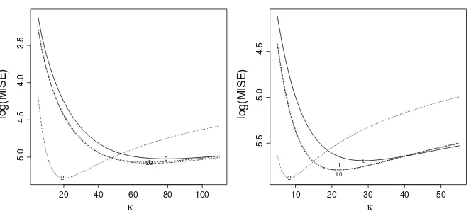
Fig. 3 log(MISE) for a range of values ofκforp=0 (solid),p=1 using Eq. (8) (dashed),L0(dotdash) andp=2 using Eq. (12) (dotted) for 200 samples of sizen=500 from equal mixture of a WC(0,0.225) and a uniform distribution (left) and an equal mixture ofvM(±π/3,5)(right)

population model is not as well behaved as a von Mises one as it has very thick tails, and the integral of the squared second derivative is larger. In such a context, we may expect that the case p =2 would be superior to other models. Simulations confirm that this is indeed the case; see Fig.3. The second example uses a equal mixture of von Mises densities to form a bimodal distribution. In this case, also, p = 2 is the best, with p=0 the worst.

The final experiments are designed to gain knowledge about practical performance in the case that the smoothing degree is data-driven. We consider sixteen models, eight of which are bivariate. They are unimodal or multimodal and are more or less (rotationally) symmetric around the origin. We use, for each sample, two bandwidth selectors: the maximizer of likelihood cross-validation (LCV) given by Eq. (4) (which uses an un-normalized estimator); and classical least-squares cross-validation (LSCV). Computations were made using MATLAB, and some example code is available fromhttp://www1.maths.leeds.ac.uk/~charles/TESTpaper/matlab.zip. The results are presented in terms of average integrated squared errors evaluated using normalized estimates; see Tables1(univariate populations) and2(bivariate populations). After noting that the relative merits of the estimators do not depend on which selector has been used, the main message is that the standard kernel is the worst density estimator, even with n = 100, when asymptotic performance is not relevant. First-order fits, i.e.P1, always have satisfactory performance because the bias reduction at the peaks,

which is mainly due to normalization, is often decisive. From additional results not reported in Table1, it appears that estimatorL0seems better suited thanP1when the

population shape is simpler but their performances are very similar.

Quadratic modelling behaves unexpectedly well, being the best one in the majority of cases. In general, it is more efficient when the roughness is more pronounced. Indeed, in the case of the uniform population, which can be considered as a proper counterex-ample in that all derivatives are zero,P0andP1fits have very similar behaviour (for

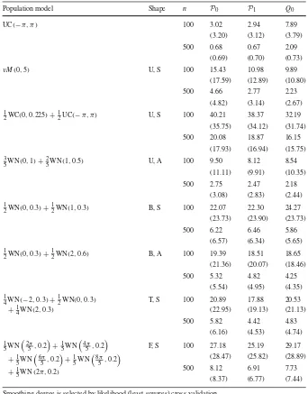
Table 1 Average integrated squared errors (1000×) over 200 samples of sizes 100 or 500 drawn from various univariate population models (WNwrapped normal)

Population model Shape n P0 P1 Q0

UC(−π, π) 100 3.02 2.94 7.89

(3.20) (3.12) (3.79)

500 0.68 0.67 2.09

(0.69) (0.70) (0.73)

vM(0,5) U, S 100 15.43 10.98 9.89

(17.59) (12.89) (10.80)

500 4.66 2.77 2.23

(4.82) (3.14) (2.67) 1

2WC(0,0.225)+12UC(−π, π) U, S 100 40.21 38.37 32.19 (35.75) (34.12) (31.74) 500 20.08 18.87 16.15

(17.93) (16.94) (15.75) 3

5WN(0,1)+25WN(1,0.5) U, A 100 9.50 8.12 8.54 (11.11) (9.91) (10.35)

500 2.75 2.47 2.18

(3.08) (2.83) (2.44) 1

2WN(0,0.3)+ 1

2WN(1,0.3) B, S 100 22.07 22.30 24.27 (23.73) (23.90) (23.73)

500 6.22 6.46 5.86

(6.57) (6.34) (5.65) 1

2WN(0,0.3)+12WN(2,0.6) B, A 100 19.39 18.51 18.65 (21.36) (20.07) (18.46)

500 5.32 4.82 4.25

(5.54) (4.95) (4.35) 1

4WN(−2,0.3)+12WN(0,0.3) +1

4WN(2,0.3)

T, S 100 20.89 17.88 20.53

(22.95) (19.13) (21.13)

500 5.82 4.42 4.83

(6.16) (4.53) (4.74) 1

5WN

2π 5,0.2

+1 5WN

4π 5 ,0.2

+1 5WN

6π 5,0.2

+1 5WN

8π 5 ,0.2

+1

5WN(2π,0.2)

F, S 100 27.18 25.19 29.17

(28.47) (25.82) (28.89)

500 8.12 6.91 7.73

(8.37) (6.77) (7.44) Smoothing degree is selected by likelihood (least-squares) cross-validation

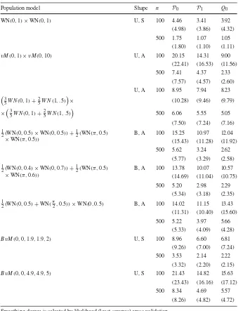
Table 2 Average integrated squared errors (1000×) over 200 samples of sizes 100 or 500 drawn from various bivariate population models (BvMstands for bivariate von Mises by Singh et al. (2002))

Population model Shape n P0 P1 Q0

WN(0,1)×WN(0,1) U, S 100 4.46 3.41 3.92

(4.98) (3.86) (4.32) 500 1.75 1.07 1.05

(1.80) (1.10) (1.11)

vM(0,1)×vM(0,10) U, A 100 20.15 14.31 9.00 (22.41) (16.53) (11.56) 500 7.41 4.37 2.33

(7.57) (4.57) (2.60) U, A 100 8.95 7.94 8.23

3

5W N(0,1)+25W N(1, .5)

× (10.28) (9.46) (9.79)

×3

5W N(0,1)+25W N(1, .5)

500 6.06 5.55 5.05 (7.50) (7.24) (7.16) 1

2(WN(0,0.5)×WN(0,0.5))+ 1

2(WN(π,0.5) ×WN(π,0.5))

B, A 100 15.25 10.97 12.04 (15.43) (11.28) (11.92) 500 5.62 3.24 2.62

(5.77) (3.29) (2.58) 1

2(WN(0,0.4)×WN(0,0.7))+12(WN(π,0.5) ×WN(π,0.6))

B, A 100 13.78 10.07 10.57 (14.69) (11.04) (10.75) 500 5.20 2.98 2.29

(5.34) (3.18) (2.35) 1

2(WN(0,0.5)+WN(π2,0.5))×WN(0,0.5) B, A 100 14.02 11.15 13.43 (11.31) (10.40) (15.60) 500 5.22 3.97 5.66

(5.33) (4.09) (4.28)

BvM(0,0,1.9,1.9,2) U, S 100 8.96 6.60 6.81

(9.26) (7.00) (7.24) 500 3.53 2.14 2.22

(3.32) (2.20) (2.15)

BvM(0,0,4.9,4.9,5) U, S 100 21.43 14.82 15.63 (23.43) (16.16) (17.12) 500 8.34 4.69 5.57

(8.26) (4.82) (4.72) Smoothing degree is selected by likelihood (least-squares) cross-validation

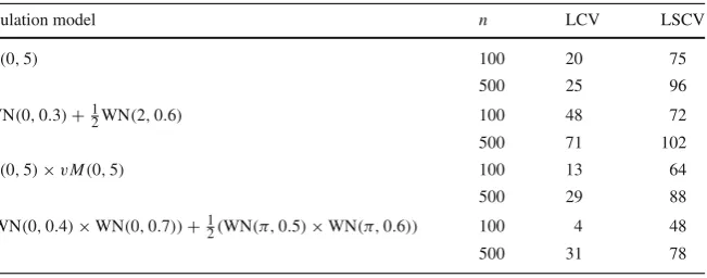
Table 3 Number of matches of estimator, over 200 samples, between optimal ISE estimator and optimal LCV (or LSCV) function

Population model n LCV LSCV

vM(0,5) 100 20 75

500 25 96

1

2WN(0,0.3)+ 1

2WN(2,0.6) 100 48 72

500 71 102

vM(0,5)×vM(0,5) 100 13 64

500 29 88

1

2(WN(0,0.4)×WN(0,0.7))+12(WN(π,0.5)×WN(π,0.6)) 100 4 48

500 31 78

Top, univariate samples; bottom, bivariate samples

The saddle-shaped population (bottom three in Table2) has large regions where the asymptotic bias is mainly due only to first-order properties of the model since sec-ond derivatives have different signs at opposite sides. In such case, variance inflation of the quadratic estimator dominates its bias reduction and the overall performance degrades. The last two models in Table2deserve particular attention because they concern correlated variables. Specifically, we use the bivariate von Mises model pro-posed by Singh et al. (2002). Similar to a bivariate Gaussian family, we have five parameters: two locations, two concentrations, and a “correlation”. Our two cases— both bimodal—are, respectively, featured by small concordance (concentrations equal to 1.9 and correlation equal to 2), and moderate concordance (concentrations equal to 4.9 and correlation equal to 5). We see that in these cases our proposals are by far superior to the standard kernel method reaching an improvement of nearly 40% in the case of moderate concordance.

A comparison between the two smoothing selectors shows that LCV performs a little better in the majority of cases, although forn =500 they appear almost equivalent. The fact that we measure discrepancy by squared errors suggests that we still could try to select at leastpby LSCV. In order to investigate the effectiveness of this approach, we have considered, for each sample of the previous simulation, the four integrated squared error curves as functions ofκ(one for each estimator), and then selected the

passociated to the smallest minimum. Then we have checked if such p is the same as the one optimizing LSCV or LCV curves overκ. In Table3we report the number of such matches for a few populations. Since the results suggest that LSCV is the best in this regard, we might thus envisage choosing the estimator based on the optimal LSCV, and then choosing the smoothing parameter for that estimator based on LCV. This idea is taken up further in the next section.

6 A real data case study

carbon–carbon) to which other atoms are linked. In particular, to one of the carbon atoms a “side chain” is formed, and the structure of this side chain defines the type of amino acid. The sequence of dihedral angles (φ, ψ, ω) along the backbone is deter-mined by the relative positions of the atoms, and this determines the overall shape of the protein after folding. Sinceωis highly predictable, with little variation, a study

of−π < φ, ψ < πis useful for many purposes, particularly in validation of newly

determined protein structures.

A plot of pairs(φi, ψi),i=1, . . .—known as a Ramachandran plot—for any

pro-tein reveals several subgroups, and mixture models of von Mises distributions have been used to summarize these from a parametric perspective. Work by Mardia et al. (2007) used an EM algorithm to fit a mixture, with the number of components being determined by AIC. Lennox et al. (2010) proposed a Dirichlet process to determine the number of components. A related Bayesian approach was developed by Boomsma et al. (2008) which allowed for many more components in a hidden Markov model, in which mixtures were trained on a set of angles from each amino acid. Kernel density estimation has also been used on the protein data (Taylor et al.2012) where interest lay in considering a bivariate density estimate conditional on the amino acid type. This has been considered as an alternative approach to validation (Lovell et al.

2003), in which procheck—based on histograms—is currently used. Finally, we note that Fernández-Durán and Gregorio-Domínguez (2016) have anaylzed similar datasets using trigonometric sums, with visual results that exhibit a periodic struc-ture.

In this case study, we use data from 500 high-quality, “representative” proteins available from the Richardson Laboratory.1Each protein is represented by a sequence of bivariate angles, each of which is associated with an amino acid. These are pooled together, and we thus obtain 20 datasets corresponding to the 20 amino acids. It should be noted that, within a protein, we expect observations not to be independent. However, in each of the 20 datasets we are pooling data from 500 unrelated proteins, and so strong dependence between observations in the same dataset will only occur when an amino acid occurs consecutively along the backbone; this is relatively uncommon. For each dataset, we can obtain a bivariate density estimate using the methods described in this paper, in which the smoothing parameter is selected by cross-validation. Our objective is to examine the differences in the estimates, and to see how these results may relate to previous work.

Obviously, we are unable to compare density estimates with the true densities for these data, as will be the case in any real-life application. One of the uses of den-sity estimation is to obtain information about subgroups, or clusters, within the data. This could be subsequently used in the fitting of (parametric) models, for example. A natural way to investigate this is to identify the location (and height) of local modes. The ability of our estimators to identify bumps has been discussed, by presenting extensive simulation evidence, in Di Marzio et al. (2016). This motivates our focus on such data, where amino acid distributions are partially characterized by modes. As it is customary in peak recognition, we applied two filters, a global and a local

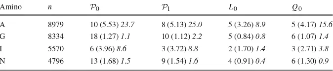
Table 4 Amino acid recognition of subgroups through bivariate density estimation

Amino n P0 P1 L0 Q0

A 8979 10 (5.53)23.7 8 (5.13)25.0 5 (3.26)8.9 5 (4.17)15.6

G 8334 18 (1.27)1.1 10 (1.12)2.2 5 (0.84)0.8 6 (1.07)1.4

I 5570 6 (3.96)8.6 3 (3.72)8.8 2 (1.70)1.4 3 (2.71)3.8

N 4796 13 (1.68)1.5 9 (1.54)1.6 4 (0.91)0.4 6 (1.30)0.9

Sample sizes, number of modes (maximum), androughnessin the estimates using various methods. The smoothing parameters are selected by likelihood cross-validation

one, in order to reduce false positives. So, for a global threshold for the modes of estimatorE ∈ {P0,P1,L0,Q0}we usedc0mEwherec0=0.005, andmEindicates

the maximum among the estimates made over an equispaced grid (of 50×50) loca-tions using E. Secondly, to avoid locations which were more akin to saddle points, we required that, at a mode, say(φm, ψm), fˆ(φm, ψm)−maxδm fˆ >c1mE, where δmrepresents the set of neighbouring points around a mode, andc1=0.0001. Table 4 gives the maximum of fˆ, the number of modes, and the roughness for some of the amino acids. It can be seen thatP0has the largest maxima and the largest

num-ber of modes, but that P1 has the largest roughness. Correspondingly, L0 has the

lowest maximum, the fewest number of modes and the smallest roughness, withQ0

generally being closer to L0. We found that the number of elements in the union of

mode locations, over all 20 amino acid datasets, for each of the methods in Table

4 is: 111, 74, 43 and 38, respectively. We note that the hidden Markov model of Boomsma et al. (2008) used 50 components in a mixture of bivariate von Mises dis-tributions which seems to be consistent with these values, except for the standard kernel.

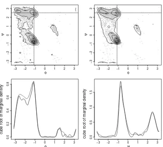
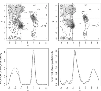
The most striking difference, however, is in the visual appearance of the density estimates, in which the difference in roughness is very evident. We first note that the height of the highest mode is much greater than the rest of the density, so in order to visualize the whole density estimate we have taken cube roots throughout. To illustrate the differences, we focus on two amino acid datasets: Alanine (A), and Asparagine (N). Figures4and5show (transformed) contour plots of estimatesP0andQ0, as well

as slices through the density estimates at the indicated values ofφandψ. The slices were chosen to pass through (or close to) a mode. Comparison of the contour plots confirms that the estimates forQ0are much smoother than those forP0. The profile

densities, which have been chosen to pass near to a local mode, show an “adaptive” smoothing character of theQ0estimate, in which the tails of the density are noticeably

smoother, while the height of the modes are not much less than those forP0. We note,

also, the possibility of spurious modes far in the tails of Q0 which may arise for

φ

ψ

−3

−2

−1

0

1

2

3

−3

−2

−1

0

1

2

3

φ

ψ

0.0

0

.2

0.4

0.6

0.8

φ

cube root of marginal density

−3 −2 −1 0 1 2 3 −3 −2 −1 0 1 2 3

−3 −2 −1 0 1 2 3 −3 −2 −1 0 1 2 3

0.0

0

.5

1.0

1.5

ψ

cube root of marginal density

Fig. 4 Top: transformed (cube-root) contour plots of the bivariate density estimates for amino acid A (alanine) usingP0(left) andQ0(right). Bottom: profile densities forP0(continuous) andQ0(dashed) corresponding toψ=2.5 (left) andφ= −1.1 (right)

7 Discussion

φ

ψ

φ

ψ

φ

cube root of marginal density

−3 −2 −1 0 1 2 3

−3

−2

−1

0

1

2

3

−3 −2 −1 0 1 2 3

−3

−2

−1

0

1

2

3

−3 −2 −1 0 1 2 3

0.0

0.2

0.4

0.6

0.8

−3 −2 −1 0 1 2 3

0.0

0.2

0.4

0.6

0.8

1.0

1.2

ψ

cube root of marginal density

Fig. 5 Top: transformed (cube-root) contour plots of the bivariate density estimates for amino acid N (asparagine) usingP0(left) andQ0(right). Bottom: profile densities forP0(continuous) andQ0(dashed) corresponding toψ=0.7 (left) andφ= −1.1 (right)

A promising development could lie in replacing our sin-polynomial expansion by a proper, flexible circular parametric family, namely the distributions based on non-negative trigonometric sums introduced by Fernández-Durán (2004) and Fernández-Durán and Gregorio-Domínguez (2016). This would give a fully para-metric method for a null concentration of the kernel, becoming more nonparapara-metric with increasing concentration. The main difficulty would be to find the global maxi-mum of the likelihood functions, which havemanylocal maxima. Kernel weighting would still be used to make the method nonparametric. The formal asymptotic theory would need to be studied, and this task appears less straightforward.

Acknowledgements The authors would like to thank the Associate Editor and two referees for their helpful comments which led to an improved version of this paper.

Appendix

Proof of Theorem1 Lettingg=log f, from Eq. (3) we have

E[ˆa] − ˜a= ˜J−1

E

1

n

n

i=1

A(θi −θ)Kκ1,...,κd(θi−θ)

−

[−π,π)d

A(α−θ)K_κ1,...,κd(α−θ)exp

˜

Pp(α−θ)

dα

⎞ ⎟ ⎠

= ˜J−1

[−π,π)d

A(α−θ)K_κ1,...,κd(α−θ)

×exp(g(α))−exp

˜

Pp(α−θ)

dα.

Observe that

exp(g(α))−exp

˜

Pp(α−θ)

=exp(g(α))

1−exp

˜

Pp(α−θ)−g(α)

≈ f(α)

g(α)− ˜Pp(α−θ)

. (15)

Hence, when pis odd, using

g(α)− ˜Pp(α−θ)=(S_α−θ)⊗(p+1) ˜ ap+1

(p+1)! +o

sinp+1

α(1)_−θ(1)_,

(16)

and f(α)= f(θ)+O

sin

α(1)_−θ(1)

in (15), due to assumption(a), we get

E[ˆa] − ˜a≈ ˜J−1

[−π,π)d

A(α−θ)K_κ1,...,κd(α−θ)f(θ)

(S_α−θ)⊗p+1a˜p₊1

(p+1)! dα

Then the bias result follows by approximating (15) along with f(α) = f(θ)+ S_α−θDf(θ)+o

sin

α(1)_−θ(1)

.

For the variance, again from Eq. (3) we see that Var[ˆa] ≈ ˜J−1VJ˜−1, whereV

stands for the covariance matrix of the LHS of system (1). We have

V= 1 n

[−π,π)d

A(α−θ)A(α−θ)K_κ2_1,...,κd(α)f(α)dα

−1 n

[−π,π)d

×

[−π,π)d

A(α−θ)_Kκ

1,...,κd(α)f(α)dα.

The second term on the RHS isO

n−111% K_κ1,...,κd(α)sin

p+1 _α(1)_dα&2_{, and}

so it is negligible under hypothesis (a). After a change of variable, the first-order

expansion for f(α)aroundθleads to the variance under assumption(b).

References

Boomsma W, Mardia KV, Taylor CC, Ferkinghoff-Borg J, Krogh A, Hamelryck T (2008) A generative, probabilistic model of local protein structure. PNAS 105:8932–8937

Delicado P (2006) Local likelihood density estimation based on smooth truncation. Biometrika 93:472–480 Di Marzio M, Panzera A, Taylor CC (2009) Local polynomial regression for circular predictors. Stat Probab

Lett 79:2066–2075

Di Marzio M, Panzera A, Taylor CC (2011) Kernel density estimation on the torus. J Stat Plan Inference 141:2156–2173

Di Marzio M, Panzera A, Taylor CC (2013) Non-parametric regression for circular responses. Scand J Stat 40:238–255

Di Marzio M, Fensore S, Panzera A, Taylor CC (2016) Practical performance of local likelihood for circular density estimation. J Stat Comput Simul 86:2560–2572

Eguchi S, Copas JB (1998) A class of local likelihood methods and near-parametric asymptotics. J R Stat Soc B 60:709–724

Fernández-Durán JJ (2004) Circular distributions based on nonnegative trigonometric sums. Biometrics 60:499–503

Fernández-Durán JJ, Gregorio-Domínguez MM (2016) CircNNTSR: an R package for the statistical analysis of circular, multivariate circular, and spherical data using nonnegative trigonometric sums. J Stat Softw 70:1–19

Fisher NI (1993) Statistical analysis of circular data. Cambridge University Press, Cambridge

Gill J, Hangartner D (2010) Circular data in political science and how to handle it. Polit Anal 18:316–336 Glad I, Hjort NL, Ushakov NG (2003) Correction of density estimators that are not densities. Scand J Stat

30:415–427

Hall P, Watson GS, Cabrera J (1987) Kernel density estimation with spherical data. Biometrika 74:751–762 Hjort NL, Jones MC (1996) Locally parametric nonparametric density estimation. Ann Stat 24:1619–1647 Lennox KP, Dahl DB, Vannucci M, Day R, Tsai JW (2010) A Dirichlet process mixture of hidden Markov

models for protein structure prediction. Ann Appl Stat 4:916–942 Loader CR (1996a) Local likelihood density estimation. Ann Stat 24:1602–1618 Loader CR (1996b) Local regression and likelihood. Springer, London

Lovell SC, Davis IW, Arendall WB, de Bakker PIW, Word JM, Prisant MG, Richardson JS, Richardson DC (2003) Structure validation by Cαgeometry:φ, ψand Cβdeviation. Proteins Struct Funct Bioinf 50:437–450

Mardia KV, Taylor CC, Subramaniam GK (2007) Protein bioinformatics and mixtures of bivariate von Mises distributions for angular data. Biometrics 63:505–512

Singh H, Hnizdo V, Demchuk E (2002) Probabilistic model for two dependent circular variables. Biometrika 89:719–723

Taylor CC, Mardia KV, Di Marzio M, Panzera A (2012) Validating protein structure using kernel density estimates. J Appl Stat 39:2379–2388