This is a repository copy of
Towards a UTP semantics for modelica
.
White Rose Research Online URL for this paper:
http://eprints.whiterose.ac.uk/105107/
Version: Accepted Version
Proceedings Paper:
Foster, Simon orcid.org/0000-0002-9889-9514, Thiele, Bernhard, Cavalcanti, Ana
orcid.org/0000-0002-0831-1976 et al. (1 more author) (2017) Towards a UTP semantics for
modelica. In: Bowen, Jonathan P. and Zhu, Huibiao, (eds.) Unifying Theories of
Programming - 6th International Symposium, UTP 2016, Revised Selected Papers. 6th
International Symposium on Unifying Theories of Programming, UTP 2016, 04-05 Jun
2016 Lecture Notes in Computer Science (including subseries Lecture Notes in Artificial
Intelligence and Lecture Notes in Bioinformatics) . Springer Verlag , pp. 44-64.
https://doi.org/10.1007/978-3-319-52228-9
[email protected] https://eprints.whiterose.ac.uk/
Reuse
Items deposited in White Rose Research Online are protected by copyright, with all rights reserved unless indicated otherwise. They may be downloaded and/or printed for private study, or other acts as permitted by national copyright laws. The publisher or other rights holders may allow further reproduction and re-use of the full text version. This is indicated by the licence information on the White Rose Research Online record for the item.
Takedown
If you consider content in White Rose Research Online to be in breach of UK law, please notify us by
Towards a UTP semantics for Modelica
Simon Foster1, Bernhard Thiele2, Ana Cavalcanti1, and Jim Woodcock1
1 Department of Computer Science, University of York, United Kingdom
{simon.foster,ana.cavalcanti,jim.woodcock}@york.ac.uk 2
PELAB, Linköping University, Sweden [email protected]
Abstract. We describe our work on a UTP semantics for the dynamic
systems modelling language Modelica. This is a language for modelling a system’s continuous behaviour using a combination of differential-algebraic equations and an event-handling system. We develop a novel UTP theory of hybrid relations, inspired by Hybrid CSP and Duration Calculus, that is purely relational and provides uniform handling of con-tinuous and discrete variables. This theory is mechanised in our Isabelle implementation of the UTP, Isabelle/UTP, with which we verify some algebraic properties. Finally, we show how a subset of Modelica mod-els can be given semantics using our theory. When combined with the wealth of existing UTP theories for discrete system modelling, our work enables a sound approach to heterogeneous semantics for Cyber-Physical systems by leveraging the theory linking facilities of the UTP.
1
Introduction
Cyber-Physical Systems (CPS) are a class of computerised system that integrate discrete computation with continuous physical processes. CPS are typically de-veloped using a combination of discrete and continuous models, often in differing heterogeneous languages. This makes verification of trustworthiness challenging. There is a need for unifying semantic models to allow the integration of heteroge-neous system components, whilst ensuring that a given set of safety properties is supported. Hoare and He’s Unifying Theories of Programming (UTP) has been designed as a framework in which the integration of languages, through the common semantic domain of the alphabetised relation calculus, can be achieved. Semantic models for discrete modelling languages in UTP are already numer-ous [26,13,36,30], and, therefore, in this paper we focus on semantics of contin-uous models in the Modelica language.
including Dymola3, Wolfram SystemModeler4, MapleSim5 and the open-source implementation, OpenModelica6. However, the Modelica language has an incom-plete formal semantics; though the semantics of DAEs is well known, the event iteration system currently does not have a formal semantics. Here we give a de-notational semantics to a fragment of Modelica using a UTP theory of hybrid relations. Additionally to clarifying the semantics of Modelica, this allows us to consider the combination of continuous and discrete models through common theoretical factors and theory linking.
Our approach to giving a semantics to Modelica is three-fold. Firstly, we create a UTP theory of hybrid relations, building on the work of He [14,15], Zhou [33,32], Zhan [21], and others. This theory extends the alphabet of UTP predicates with continuous variablesc∈conαand is defined by novel healthiness conditions that characterise these variables as piecewise continuous functions.
Secondly, we define the operators of our hybrid relational calculus, which is similar to the imperative subset of HCSP [34], but extended with an interval operator [33] that provides a continuous specification statement. In particular we provide support for semi-explicit DAEs and continous variable preemption. As with Hybrid CSP, we base the denotational semantics around the Duration Calculus [33], though the semantics is purely relational. Moreover, we provide a uniform account of both discrete and continuous variables by linking the latter to discrete “copy” variables that give the valuation at the beginning and end of a continuous evolution. Thus, both discrete and continuous variables can be manipulated with the same operators; in the latter case this provides initial value constraints. Our model of hybrid relations has also mechanised in our UTP proof assistant, Isabelle/UTP[10], that provides theorem proving facilities.
Thirdly, we define a preliminary denotational semantics for Modelica through a mapping into the hybrid relational calculus. This mapping primarily consid-ers the event-handling mechanism of Modelica, whereby specific conditions on continuous variables can lead to both discontinuous jumps in variables, and also changes to the equations active in the DAE system.
The remainder of our paper is structured as follows. In section2, we provide background on hybrid systems by briefly surveying the literature, with particular emphasis on works related to the UTP. In section3we briefly describe the UTP, and in section 4 we introduce the Modelica language. In section5, we describe our UTP theory of hybrid relations. In section 6, we use our UTP theory to build a hybrid relational calculus, including operators for specifying continuous invariants, differential equations, and preemption. In section 7, we outline our mechanisation of the hybrid relational calculus in Isabelle [23,10]. In section8, we use our hybrid relational calculus to give a high-level denotational seman-tics to the Modelica language, focusing principally on the interaction between
3
http://www.3ds.com/products-services/catia/products/dymola 4
http://www.wolfram.com/system-modeler/ 5
http://www.maplesoft.com/products/maplesim/ 6
evolution of DAEs and the event handling system. Finally in section9, we draw conclusions.
2
Related work: Hybrid Systems
The majority of the work on hybrid systems takes inspiration from Hybrid Au-tomata [16], an extension of finite state automata that allows the specification of continuous behaviour. A hybrid automaton consists of a finite set of states la-belled by ODEs, a state invariant, and initial conditions. The states (or “modes”) are connected by transitions that are labelled with jump conditions and (option-ally) events. Whilst in a state the continuous variables evolve according to the system of ODEs and the given invariant; this is known as aflow as the variable values continuously flow from one value to another. When one of the jump con-ditions of an outgoing edge is satisfied, the event, if present, can instantaneously execute, potentially resulting in a discontinuity, and the targeted hybrid state is activated. Thus a hybrid automata is characterised by behaviour that includes both continuous flows also discrete jumps. Hybrid automata are given a deno-tational semantics in terms of piecewise continuous functions [16]R→Rn, also
called trajectories, that are continuous except for in a finite number of places. Verification of hybrid systems was made possible through the seminal work of Platzer [27]. This work develops a logic called Differential Dynamic Logic (dL) that allows us to specify invariants over both discrete and continuous variables. Hybrid systems are modelled using a language of hybrid programs, that combines the usual operators of an imperative language with continuous behaviour spec-ified by differential equations. Hybrid programs are equipped with a relational semantics, and a proof calculus fordLallows reasoning about hybrid programs. An implementation of dL called KeYmaera [27] allows the automated verifica-tion of systems modelled as hybrid programs. Our noverifica-tion of hybrid relaverifica-tion is inspired by Platzer’s hybrid programs, though we focus on a UTP denotational semantics as opposed to an operational semantics. Our own setting of the Dura-tion Calculus [33] provides us with the necessary machinery to similarly justify a dynamic logic. Moreover, we observe that, with a UTP model, we are in a strong position to extend the work to deal with concurrent hybrid programs, a notion that dL does not consider.
Concurrency is considered in Hybrid CSP [14,34] (HCSP), an extension of Hoare’s process calculus CSP [17] that adds support for continuous variables as described by differential equations and modelled by standard trajectories, in a similar manner to hybrid automata. HCSP [14] extends CSP with continu-ous variables whose behaviour is described by differential equations of the form
F(˙s,s) = 0. Interaction between discrete and continuous behaviour takes the form of preemption conditions on continuous variables, timeouts, and interrup-tion of a continuous evoluinterrup-tion through CSP events. HCSP has a denotational semantics that is presented in a predicative style similar to the UTP [18].
denotational semantics in terms of the Extended Duration Calculus [35], which treats variables as piecewise continuous functions. This allows a more precise semantics for operators like preemption that are defined in terms of suitable variable limits. A Hoare logic for this calculus is presented in [21], through the adoption of Platzer’s differential invariants, along with an operational semantics. Our work is heavily influenced by HCSP, though we focus on formalising the sequential aspects of hybrid systems, and so formalise a subset of the operators with refined definitions. Our operators formalise continuous after variables by explicitly considering left-limits which is important for Modelica event iteration. A theorem prover for HCSP called, HHL Prover [37], has also been devel-oped and applied to verification of Simulink diagrams through a mapping into
HCSP [31]. More recently the fundamentals of hybrid system modelling have been studied in a purely UTP relational setting [15]. This work has produced a language called the Hybrid Relational Modelling Language [15] (HRML), which draws on HCSP, but uses signals rather than CSP’s events as the main com-munication abstraction. Our notation is agnostic in this respect, and could be extended either to support the event or signal paradigm.
Duration Calculus [33] (DC) provides specification of invariants over the con-tinuous time domain, in order to facilitate verification real-time systems. For example, we can write
x2>7
, which specifies all possible intervals of over which x2 > 7 is invariant. The chop operator P◦Q specifies that an interval may be broken into two subsequent intervals, over which P and then Q hold, respectively. DC has been extended to provide a semantics for hybrid real-time systems modelling [35], which is then used to give semantics to HCSP [34].DC
can also be used to give an account to typical operators of modal and temporal logics. Thus, grounding our semantics inDCenables us to form continuous spec-ifications about hybrid systems. Different to DC we provide a purely relational UTP semantics, and also explictly distinguish continuous and discrete variables, instead of modelling the latter as step functions. This distinction allows us to retain standard relational definitions of the majority of discrete UTP operators.
3
Unifying Theories of Programming
Concretely, an alphabetised relation is a pair(αP,P)whereαP is the alpha-bet and P is a predicate all of whose free variables belong toαP. The alpha-bet can in turn be subdivided α(P) =inα(P)∪outα(P), with input variables x,y ∈inα(P) and output variablesx′,y′ ∈outα(P). The calculus provides the
operators typical of first order logic. UTP predicates are ordered by a refinement partial orderP ⊑Qthat also defines a complete lattice. Imperative programs can be described using relational operators, such as sequential composition P ; Q, if-then-else conditional P
2
b3
Q, assignment x :=A v (for expression v and alphabetA), and skipIIA, all of which are given predicative interpretations.More sophisticated language constructs can be expressed by enriching the theory of alphabetised relations to create UTP theories. A UTP theory consists of (i) a set of observational variables, (ii) a signature, and (iii) a set of healthiness conditions. The observational variables record behavioural semantic information about a particular program. For example, we may have an observational vari-able for recording the current time called clock : R. The signature uses these
operational variables to encode the main operators of the target language. The domain of a UTP theory can be constrained through healthiness con-ditions, which act as invariants over the observational variables. For example, it is intuitively the case that time only moves forward, and so a relational ob-servation like C , clock = 3∧clock′ = 1 ought not to be possible. We can
eliminate this kind of behaviour description with an invariant clock ≤ clock′.
In the UTP such conditions are expressed as idempotent functions, for example
HT(P) = P ∧clock ≤ clock′, so that healthiness of a predicate P can be
ex-pressed as a fixed point equation:P =HT(P). If we applyHT toC, the result
is miraculous predicatefalse and thusC is excluded from the theory signature.
UTP theories can be used to describe a domain useful for modelling partic-ular problems – for instance, we can add further conditions to HT to provide
a theory of real-time programs. UTP theories can also be composed to produce modelling domains that combine different language aspects. Put more simply, UTP theories provide the building blocks for a heterogeneous language’s denota-tional semantics [9]. Such a denotational semantics provides the “gold standard” for the meaning of language constructs and can then be used to derive other presentations, such as operational and, very often, algebraic.
4
Modelica
Modelica Model
Flat Modelica (Hybrid DAE)
Simulation Result
Modelica Specification
Mathematical denotation for hybrid DAE system
Fig. 1. From model to simulation result.
m o d e l B o u n c i n g B a l l Real h ; Real v ;
i n i t i a l e q u a t i o n
h = 1.0;
e q u a t i o n
v = der( h ) ;
der( v ) = -9.81;
w h e n h <0 t h e n
reinit ( v, -0.8*pre( v ) ) ;
end w h e n;
end B o u n c i n g B a l l ;
Fig. 2.Bouncing ball in Modelica.
Fig.1illustrates the basic idea. The squiggle arrow denotes a degree of fuzzi-ness — a simulation result is an approximation to the, in general, inaccessible exact solution of the equation system and the specification does not prescribe a particular solution approach. A classical model for a hybrid systems is the bouncing ball. A possible Modelica implementation for a ball with mass 1kg and an impact coefficient of 0.8 that falls from an initial height of h = 1m is given in Fig. 2. When the ball hits the ground, it changes its velocityv discon-tinuously and bounces back. der(h)and der(v)denote the time derivativesh˙ and v˙ of variablesh and v, respectively. The acceleration to the ground is de-termined by earth’s gravitational accelerationg= 9.81m/s2. The discontinuous change of variablev is modelled using a conditionally activated reinitialization equation. The ball hits the ground when condition h < 0 becomes true. The reinit()operator is used for reinitializingvwith the negative value ofv(times the impact coefficient) just before conditionh<0becomes true (pre(v)returns the left limit of variablev at the event instant).
Several formal specification approaches have been used to give semantics to subsets of the Modelica language. Most of the approaches describe the instantia-tion and flattening of Modelica models (i.e.,thestatic semantics, corresponding to the first stage in Fig.1) [20,1,28] while others are restricted to discrete-time language subsets [29].
Flat Modelica can be conceptually mapped to a set of differential, algebraic and discrete equations of the following form [22, Appendix C]:
1. Continuous-time behaviour. The system behaviour between events is de-scribed by a system of differential and algebraic equations (DAEs):
f x(t),x(t),˙ y(t),t,m(te),mpre(te),p,c(te)
= 0 (1a)
g x(t),y(t),t,m(te),mpre(te),p,c(te)
= 0, (1b)
derivatives;y(t) is a vector of algebraic variables of type Real; m(te) is a vector of discrete-time variables of typediscrete Real,Boolean,Integer, or Stringwhich changes only at event instants te; mpre(te)are the values
ofm immediately before the current event at event instantte; andc(te)is a vector containing all Boolean condition expressions,e.g., if-expressions. 2. Discrete-time behaviour.The behaviour at an event at time te is described
by following discrete equations:
m(te) :=fm x(te),x(te),˙ y(te),mpre(te),p,c(te)
(2)
c(te) :=fe mB(te),mBpre(te),pB,rel(v(te))
. (3)
An event fires if any of the conditions c(te) change from false to true.
The vector-valued functionfm specifies new values for the discrete variables m(te). The vectorc(te)is defined by the vector-valued functionfe, which con-tains allBooleancondition expressions evaluated at the most recent eventte; rel(v(te)) =rel([x(t); ˙x(t); y(t); t; m(te); mpre(te); p])is a Boolean-typed
vector-valued function containing variablesvi,e.g., v1>v2,v3≥0;mB(te) is a vector of discrete-time variables of typeBoolean,mB(te)⊆m(te), and mB
pre(te)are the values ofmBimmediately before the current event at event
instantte;pBare parameters and constants of typeBoolean,pB⊆p.
Simulation means that an initial value problem (IVP) is solved. The equations define a DAE which may have discontinuities and a variable structure and may be controlled by a discrete-event system.
5
Theory of Hybrid Relations
We now proceed to describe our theory of hybrid relations to enable the def-inition of a relational calculus for modelling sequential hybrid processes. Our model unifies the treatment of discrete and continuous variables so that the same operators may be used for manipulating both. In Modelica, DAEs are used to describe continuously evolving dynamic behaviour of a system. Thus, in the UTP, we first introduce a theory of continuous time processes that embeds tra-jectories into alphabetised predicates and shows how continuous variables evolve over a given interval. These intervals are used to divide up the evolution of a system into piecewise continuous segments.
Our theory is based on vanilla UTP alphabetised relations, and so is insen-sitive to termination and stability of continuous processes. Following the UTP philosophy, we consider hybrid behaviour in isolation, and then later augment it with additional structure to allow the finer expression of such properties. Our theory can, for instance, be embedded into timed reactive designs [13,30].
Alphabet. Our model of continuous time introduces observational variables ti, ti′:R
As already said, the alphabetised relational calculus divides the alphabet into input inα(P)and output variables outα(P). Inspired by [15], we add a further subdivisionx,y,z∈conα(P), the set of continuous variables, that is orthogonal to the discrete program variables, that is conα(P)∩(inα(P)∪outα(P)) = ∅. The elements of conα(P)are the variables to be used in differential equations and other continuous constructs.
We assume that all variables consist of a name, type, and optional deco-ration. For example, the name in the variables x, x′, and x is the same – x
– but the decorations differ. We introduce the distinguished continuous vari-able t that denotes the current instant in an algebraic or differential equa-tion. An alphabetised predicate P whose alphabet can be so partitioned, i.e. α(P) =inα(P)∪outα(P)∪conα(P), is called ahybrid relation.
Continuous variables come in two varieties that allows us to talk about a particular instant or about the whole time continuum:
– instant variables – these are continuous variables of typeRthat refer to the
value at a particular instant;
– trajectory variables – these are time-dependent variables of typeR≥0 →R
and give the values over a whole trajectory.
Trajectory variables are total rather than partial functions. This has the ad-vantage that composition operators need not consider explicit combination of trajectories through overriding. Instead, composition further constrains the tra-jectory functions, potentially over disjoint time domains (as is the case for ;). Valuations of the trajectory exist outside[ti, ti′), but they have no relevance.
We require that each trajectory variable x : R≥0 → R is accompanied by
discrete before and after “copy” variables with the same name –x,x′:R– that
record the values at the start and limit of the current interval. This, crucially, allows us to use the standard operators of relational calculus for manipulating continuous variables via discrete copies. This allows us to consider the set of purely discrete variables that are not discrete copies of a continuous variable:
disα(P) ={x∈inα(P) | x∈/conα(P)} ∪ {x′ ∈outα(P) | x ∈/ conα(P)}
We introduce the following @ operator borrowed from [6] that lifts a predicate in instant variables to one in trajectory variables.
Definition 1. Continuous variable lifting
P@τ,{x7→x(τ) | x ∈conα(P)\ {t}} †P
The dagger (†) operator is a nominal substitution operator. It applies the given partial function, which maps variables to expressions, as a substitution to the given predicate, so thatP[v/x] ={x7→v} †P. We construct a substitution that maps every flat continuous variable (other than the distinguished time variable t ∈[ti..ti′)) to a corresponding variable lifted over the time domain. The effect
of this is to state that the predicate holds for values of continuous variables at a particular instantτ, a variable that is potentially free inP. Each flat continuous variablex:T is thus transformed to have a time-dependent functionx:R→T
P,Q::= P;Q | P
2
b3
Q | x:=e | P∗ | Pω | ⌈⌈P⌉⌉ | hFn|bi | P[b]QTable 1.Signature of hybrid relational calculus
Healthiness conditions. We introduce two healthiness conditions:
HCT1(P),P∧ti≤ti′
HCT2(P),P∧
ti < ti′⇒ ^
v∈conα(P)
∃I :Roseq •ran(I)⊆ {ti . . . ti′} ∧ {ti, ti′} ⊆ran(I)∧
∧(∀n<#I−1•
v cont-on[In,In+1))
where
Roseq , {x :seqR | ∀n<#x−1•xn<xn+1}
f cont-on[m,n) , ∀t ∈[m,n)•lim
x→tf(x) =f(t)
HCT1states that time may only ever go forward, as should be the case, and thus
the time interval is well-defined.HCT2 states that every continuous variablev
should be piecewise continuous, that is, that for non-empty intervals there exists a finite number of points (range of I) between tiand ti′ where discontinuities
occur. We define the set of totally ordered sequencesRoseq that captures this set
of discontinuities, and the continuity off is defined in the usual way by requiring that at each point in[ti, ti′), the limit correctly predicts where the function goes.
HCT1 andHCT2 are idempotent, monotone, and commutative as they are
both conjunctive. We then have thatHCT =HCT2 ◦ HCT1 also satisfies all
these properties. Furthermore it defines a complete lattice.
Theorem 1. HCT predicates form a complete lattice under d and F
, with
⊤H =HCT(true) and⊥H =false.
Proof. By conjunctivity of HCT. Properties of conjunctive healthiness
condi-tions are proved in [12]. ⊓⊔
6
Hybrid relational calculus
The signature of our theory is given in Table1. It consists of the standard oper-ators of the alphabetised relational calculus together with operoper-ators to specify intervals⌈⌈P⌉⌉, differential algebraic equationshFn|bi, and preemptionP[b]Q. Using this calculus, we can describe the bouncing ball example from Fig.2:
Example 1. Bouncing ball in hybrid relational calculus
h,v:= 1,0;Dh˙ =v; ˙v=−9.81E[h<0 ]v:=−v·0.8)ω
Example 2. Cartesian pendulum in hybrid relational calculus
D
˙
x=u; ˙u=λ·x; ˙y =v; ˙v=λ·y−9.81 x
2+y2=l2E
This system consists of four differential and one algebraic equation in terms of the position(x,y), horizontal and vertical velocities u andv, and the length l of the pendulum cable. The differential equations describe the horizontal and vertical components of the pendulum’s movement vector, governed by the laws of conservation of energy and gravity using a constant λ previously defined. The algebraic equation tiesxandytogether through the Pythagorean theorem, ensuring that the length of the cable must be respected by the movement. ⊓⊔
We note that many of the standard operators of the alphabetised relational calculus retain their standard denotational semantics [18] in this setting, but over the expanded alphabet. Indeed, an alphabetised relation is simply a hybrid relation with the degenerate alphabet conα(P) = ∅. For continuous variables, sequential composition behaves like conjunction. In particular, if we haveP;Q, withPandQrepresenting evolutions over disjoint intervals, then their sequential composition combines the corresponding trajectories when they agree on variable valuations. Put another way, the final condition of P also defines the initial condition forQ as in the Z schema composition operator.
Similarly, other operators like the Kleene star and Omega iteration operators P∗ andPω, being defined solely in terms of sequential composition, disjunction
(internal choice),II, and fixed point operators, also remain valid in this context. Thus we already have the core operators of an imperative programming language at our disposal. We prove that these core operators satisfy our two healthiness conditions in Isabelle (cf. section7), but for now we state the following theorem.
Theorem 2. The following operators of relational calculus P ; Q, P
2
b3
Q,P∗,II, x:=v, and falseare HCTclosed.
The maximally nondeterministic relationtrueis of course notHCT healthy, and
so we supplement our theory withtrueH ,HCT(true). We define the interval
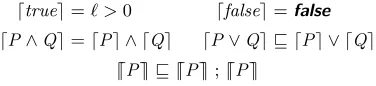
operator fromDC[33] and our own variant.
Definition 2. Interval operators
⌈P⌉ , HCT2(ℓ >0 ∧ (∀t∈[ti, ti′)• P@t))
⌈⌈P⌉⌉ , ⌈P⌉ ∧ ^
v∈conα(P)
(v=v(ti)∧v′ = lim
t→ti′(v(t)))∧IIdisα(P)
⌈P⌉ is a continuous specification statement thatP holds at every instant over all non-empty right-open intervals fromtitoti′; it corresponds to the standard
DC operator. We apply HCT2 to ensure that all variables are also piecewise
⌈true⌉=ℓ >0 ⌈false⌉=false
⌈P∧Q⌉=⌈P⌉ ∧ ⌈Q⌉ ⌈P∨Q⌉ ⊑ ⌈P⌉ ∨ ⌈Q⌉
[image:12.612.214.402.101.144.2]⌈⌈P⌉⌉ ⊑ ⌈⌈P⌉⌉;⌈⌈P⌉⌉
Table 2.Algebraic laws of durations
condition of each continuous variable x in the interval is constrained by the valuation of the corresponding discrete copy x. Likewise, the condition at the limit of the interval is recorded in the corresponding discrete after variablex′.
Crucially, this provides a uniform view of discrete and continuous variables when handled over an interval, and allows the use of standard relational opera-tors for their manipulation. Moreover, by taking the limit rather than the final value of a continuous variable we do not constrain the trajectory valuation atti′
meaning it can be defined by a suitable discontinuous discrete assignment at this instant. Following [14] we ground our definition of differential equation systems in this interval operator. This will, for example, allow us to formally refine a DAE, under given initial conditions, to a suitable solution expressed using the interval operator. Intervals satisfy a number of standard laws ofDC illustrated in Table2, which we prove in section7.
We next introduce an operator, adapted fromHCSP [34,21], to describe the evolution of a system of differential-algebraic equations.
Definition 3. DAE system in semi-explicit form
hv˙1=f1; · · · ; ˙vn =fn|0 =b1; · · ·; 0 =bmi
,⌈⌈(∀i∈1..n,∀j∈1..m• v˙i(t) =fi(t,v1(t),· · · ,vn(t),w1(t),· · · ,wm(t)))
∧ 0 =bj(t,v1(t),· · ·,vn(t),w1(t),· · ·,wm(t))⌉⌉
A DAE hFn|Bmi consists of a set of n functions fi : R×Rn×Rm →Reach of which defines the derivative of variable vi in terms of the independent time variablet andn+m dependent variables. It also contains algebraic constraints bj : R×Rn ×Rm → R that must be invariant for any solution and do not
refer to derivatives. For m = 0 the DAE corresponds to an ODE, which we write as hFni. The DAE operator is defined using the interval operator to be all non-empty intervals over which a solution satisfying both the ODEs and algebraic constraint exists. Non-emptiness is important as it means that a DAE must make progress: it cannot simply take zero time sinceℓ >0, and so a DAE cannot directly cause “chattering Zeno” effects when placed in the context of a loop, though normal Zeno effects remain a possibility.
As previously explained, at the initial time (ti) each continuous variableviof the system is equated to the value of the corresponding discrete input variablevi. To obtain a well defined problem description, we require the following conditions to hold [2]: (i) the system of equations is consistent and neither underdetermined nor overdetermined; (ii) the discrete input variablesvi provide consistent initial conditions (ICs7); (iii) the equations are specific enough to define a unique solu-tion during the intervalℓ. The system is then allowed to evolve from this point in
7
Notice that in the general case ICs for DAE systems may actually involve derivatives
˙
the interval betweentiandti′ according to the DAEs. At the end of the interval,
the corresponding output discrete variables are assigned. During the evolution all discrete variables and unconstrained continuous variables are held constant.
Finally, we define the preemption operator, adapted fromHCSP.
Definition 4. Preemption operator
P[B]Q,(Q
2
B@ti3
(P∧ ⌈¬B⌉))∨((⌈¬B⌉ ∧B@ti′∧P);Q)Intuitively,P is a continuous process that evolves until the predicate B is sat-isfied, at which pointQ is activated. This operator is used to capture events in Modelica. The semantics is defined as a disjunction of two predicates. The first predicate states that, if B holds in the initial state of ti, then Q is activated immediately. Otherwise, P is activated and can evolve while B remains false (potentially indefinitely). The second predicate states that ¬Bholds on the in-terval[ti, ti′)until instantti′, whenB switches to a true valuation; during that
invervalP is executing. Following this,P is terminated andQ is activated.
7
Mechanisation in Isabelle/UTP
Our Isabelle [23] mechanisation serves two purposes: firstly it validates the model by enabling us to prove algebraic laws, and secondly it enables theorem proving for hybrid programs. It is based in a shallow embedding of the UTP8, which provides direct proof automation through a combination of Isabelle/Circus [5] and our own deep model [10]. UTP relations are represented by predicates over bindings, and bindings over a given alphabet are represented using record types, where each field corresponds to a variable. The model is based on a UTP ex-pression type(′a, ′α)uexpr ranging over alphabet type ′αand with return type ′a. Alphabetised predicates ′αupredare expressions with a boolean return type,
and relations are predicates over a product type(′α× ′β)upred.
We mimic the syntax of UTP predicates as given in most standard publica-tions (e.g. [18,4]). Where this is not possible, we supplement the same syntax with an added subscriptu. For example, equality in Isabelle “=” denotes HOL equality, so we use =u for UTP equality. Input variable and output variable expressions are written $x and$x´ respectively. We also make use of Isabelle’s implementation of Cauchy real numbers and analysis [7,11]. Our proofs make heavy use of Isabelle’s automated proof facilities likeautoandsledgehammer[3]. This has allowed us to use Isabelle to validate the healthiness conditions and definitions given in the previous sections. We prove that they respect appro-priate laws, which increases confidence in the correctness of our UTP theory.
finding consistent ICs from “guess” values exist [2,24]. However, numerical/symbolic methods for solving IVPs is not within the scope of our current work. Hence, we only consider less general ICs and presume that consistent ICs are provided. 8
This section has been compiled using Isabelle’s document preparation system: all definitions and theorems have been mechanically verified9.
record(′d, ′c)hyst = stateu :: ′d × ′c timeu ::real traju ::real ⇒ ′c
type-synonym(′d, ′c)hyrel = (′d, ′c)hyst hrelation
A hybrid state (′d, ′c) hyst represents the alphabet, or equivalently the state
of the hybrid relation, at a particular instant. We represent this using a record with three fields: stateu denoting the state variables,timeu denoting the time, and traju denoting the trajectory of continuous variables. The record type is parametrised by the discrete portion of the alphabet, denoted by type ′dand the
continuous portion denoted by type ′c. The state field’s type is a product of the
discrete and continuous state, whilst the trajectory refers only to the continuous state. Intuitively, this encodes the distinction between discrete and continuous variables. A hybrid relation is then a homogeneous relation (hrelation) over the hybrid state. We next give the healthiness conditions of our theory.
definitionHCT1(P) = (P ∧$time ≥u 0 ∧ $time≤u $time´)
HCT1 is broadly the same as in section6, though we additionally require that the initial time be no less than zero; this is due to our use of the standard type real that also encompasses negative numbers.
definitionHCT2(P) = (P ∧($time´>u $time ⇒
(∃ I ·{$time,$time´}u⊆u ranu(I)∧ranu(I) ⊆u {$time ..$time´}u ∧(∀ n· n<u #u(I) −1 ⇒$traj cont−onu {I(|n|)u ..<I(|n+1|)u}u)
∧sortedu(I)∧distinctu(I))))
HCT2 also explicitly requires that the trajectory sequenceI is both sorted and distinct, which equates to it being linearly sorted as required.
definitionHTRAJ(P) = (P ∧$traj =u $traj´)
We also have to add an auxiliary healthiness condition HTRAJ. This allows us to use standard HOL binary relations, where there is only inputs and outputs, to represent hybrid relations. Specifically, we have two copies of the trajectory, a before version and an after version and so this healthiness condition ensures the trajectory remains constant throughout. Monotonicity and idempotence of the healthiness conditions is proved by our automated relational calculus tactic.
With our healthiness conditions defined, we can proceed to define the opera-tors. The basic operators, such asIIand @ are elided here, and we instead focus on the continuous operators. We first define the two interval operators.
definition
9
hInt P =HCT($time´>u $time ∧(∀ t ∈ {$time ..<$time´}u ·P •u t))
Definition hInt corresponds to the interval operator ⌈P⌉, and has an almost identical definition. In our mechanisation, an interval can be written as ⌈P⌉H whereP is a predicate with the time variableτ free.
definition
hDisInt P = (hInt P ∧ π1($state´) =u π1($state)∧π2($state) =u $traj(|$time|)u ∧π2($state´) =u limu(x →$time´−)($traj(|x|)u))
Our modified interval operator ⌈⌈P⌉⌉, represented here by hDisInt conjoins the standard interval operator with predicates that ensure that discrete variables remain const and and that continuous variable copies match the initial value in the trajectory, and the left limit of the trajectory at the end. Here πn is a function that returns the nth element of a product, fLxMu represents function application, and limu(x →t−) denotes the left-limit. This interval operator is
written⌈|P |⌉H, again withτ free.
Next we define the operators for ODEs and DAEs. The first step is to for-mally mechanise the notion of time derivatives ( ˙x). Thus we define a predicate hasDerivAtthat relates ODEs to solution functions using the lifting package [19].
type-synonym ′c ODE =real × ′c ⇒ ′c
lift-definitionhasDerivAt ::
(real ⇒ ′c ::real-normed-vector)⇒ ′c ODE ⇒real ⇒(′a, ′b)relation
(- has−deriv - at -[90,0,91]90)
isλF F′τ A.(F has-vector-derivative (F′(τ ,F τ))) (at τ within {0..}) .
An explicit system of ODEs (′c ODE) is encoded as a functionreal × ′c ⇒ ′c,
where the real is the time parameter, and ′c is a vector of real variables. We
require that ′cbe within the type classreal-normed-vector of real vector spaces.
Isabelle’s Multivariate Analysis library contains a functionhas-vector-derivative that relates a solution functionF:R→Rn with its deriativesF˙ :Rn at instant
τ within a particular range. It represents the Fréchet derivative of differential equations in a vector space. We use this to define a construct F has−deriv F′
at τ whereF is a solution function,F′is the system of ODEs. This predicate is
accompanied by a large number of rules that can be used to certify derivatives of polynomial functions. We now use these to encode operators for ODEs, DAEs, and ODEs under an initial condition.
definition hF′iH = (∃ F · ⌈| F has−derivF′atτ ∧&conα=u F(|τ|)u|⌉H)
definition hF′|Bi
H = (hF′iH ∧ ⌈|B|⌉H)
definition I |=hF′iH = (hF′iH ∧$traj(|$time|)u =uI)
We choose to implement ODEs and DAEs as separate constructs, as the defini-tions are simpler, though equivalent to those in the previous section. An ODE
hF′i
H specifies that a solution functionF to the given ODE must exist and that at each point of the interval the values of all continuous variables (conα) track this solution function. A DAEhF′|Bi
of ODEs as explicit initial value problems by I |= hF′i
H where I gives initial values to all continuous variables.
Finally, we prove some key laws about our hybrid relational calculus. Firstly we show that sequential composition isHCT closed, which partly validates our healthiness conditions with respect to the standard relational calculus. This is proved by an apply-style Isabelle proof which is omitted.
theorem seq-r-HCT-closed:
assumesP is HCT andQ is HCT
shows(P ; ; Q)is HCT
by(metis HCT-seq-r Healthy-def′assms(1) assms(2))
In order to demonstrate the use of ODEs in this framework, we take the ODE from the bouncing ball example, and show how its solution can be expressed as a refinement statement.
theorem gravity-ode-refine:
((v0,h0)u |=hλ(t,v,h).(−g,v)iH ∧ $time =u 0)⊑
(⌈|&conα=u (v0 −g·τ ,v0·τ −g·(τ·τ)/2 +h0)u |⌉H ∧$time =u 0)
by(rel-tac ; rule exI ; auto; vderiv-tac)
As in Example 1, we specify the ODE with two variables, v and h that will give the velocity and height about the ground of the ball. We refine this in the window time = 0 as it makes the solution simpler via an appropriate conjunction. Given initial conditions of v0 and h0 for the respective variables, solutions to the ODE equations arev0−g·τand(v0·τ−g·τ2)/2+h0, respectively. The solutions are proved correct in Isabelle automatically by application of our relational calculus tactic rel-tac, followed by existential introduction (exI) to introduce the ODE solution, application of the auto tactic, and then finally application of our own tactic vderiv-tac. This tactic recursively applies the set of introduction for differentiation in an effort to show that a given ODE is the derivative of a given solution. This example serves to demonstrate how a theorem prover can reason about differential equations in terms of their solution intervals making use of refinement and the Duration Calculus.
8
Modelica Semantics
In this section we give a semantics for flat Modelica whose models are given by a set of conditional differential, algebraic, and discrete equations. More specifi-cally, we assume that a Modelica model consists of a set of dynamic variablesx, algebraic variablesy, and discrete variablesq, and
– a set ofk∈N>0conditional DAEs, consisting of: • differential equationsx˙ =Fi(x,y,q)fori∈1..k;
• algebraic equationsy=Bi(x,y,q)fori∈1..k;
initialisation or the previous event. We assume that at least one set of equations is active at any time;
– a set ofl ∈N boolean event conditions Ci(x,y,q) for i ∈ 1..l, that trigger
an event when changing value. These must be specified in terms of the core Modelica relational operators, namely≤,<,=, and6=;
– a set ofm ∈Nconditional discrete equation blocks, consisting of:
• n boolean discrete-event guardsHi,j(x,y,q,qpre)fori∈1..m,j∈1..n; • n discrete equations / algorithmsPi,j(x,y,q,qpre)fori∈1..m,j∈1..n.
We assume the discrete equations are sorted into a suitable sequence.
Each conditional DAE describes a possible continuous behaviour using a col-lection of differential and algebraic equations. The particular behaviour to be executed is chosen based on the evaluation of the guards, which take as input the valuations of the discrete and continuous variables at the (re)start of the continuous evolution. The possible events that can occur are described by a collection of boolean event conditions, which act as guards that can stop the continuous evolution. Once one or more of these guards changes value an event is fired, and possible discrete behaviour is executed. Usually such guards are implemented in terms of a zero crossing function, though our semantics specifies them abstractly. The appropriate discrete behaviours are then chosen through a collection of discrete event guards, and the resulting behaviour by an appropriate discrete equation that may be specified by a suitable algorithm.
M = Init;(DAE[Events]Discr)ω
Init = x,y,q:=u,v,w
DAE =
x=F1( ˙x,y,q)
B1(x,y,q)
2
G13
· · ·2
Gn−13
˙
x=Fn(x,y,q)
Bn(x,y,q)
Events = _
i∈{1..k}
Ci(x,y,q)6=Ci(x,y,q)
Discr = varqpre •
untilqpre=qdo
qpre:=q;
P1,1(x,y,q,qpre)
2
H1,1(x,y,q,qpre)3
P1,2(x,y,q,qpre)2
· · ·;· · ·; [image:17.612.142.485.395.589.2]Pm,1(x,y,q,qpre)
2
Hm,1(x,y,q,qpre)3
Pm,2(x,y,q,qpre)2
· · ·; odFig. 3.Overall semantics of a Modelica modelM
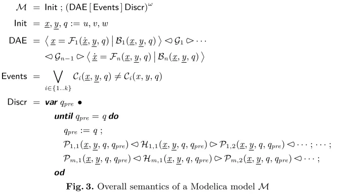
We give the semantics for such a Modelica model M, which is shown in Fig.3, in terms of four main definitions.
DAE denotes the conditional system of differential and algebraic equations active during the continuous evolution of the model. It is represented by a con-ditional predicate that selects an appropriate set of differential and algebraic equations based on initial values of discrete and continuous variables.
Events denotes the event preemption condition, and is a disjunction of all possible event conditions (“relations” in Modelica terminology) in the Modelica model. In this way, the DAE remains active until one of the event conditions changes from its initial value, at which point it is preempted.
Finally, Discr describes possible discrete behaviour to be executed during event iteration; a finite event loop adapted from the pseudo code given on page 263 of [22]. The initial value of all discrete variables is first copied by creation of a local variable qpre that holds the initial value of q. Each conditional discrete equation is then evaluated, which may lead to updates to q, and then the pro-cedure iterates. The event iteration terminates when no more updates to q are made: a fixed point is reached. In Modelica the existence of a fixed point is not guaranteed and event iteration can potentially lead to an infinite loop.
To illustrate, we use the bouncing ball Modelica example from Fig.2. It has continuous variables representing the height of the ball above the groundhand the velocity of the ball v. For giving a semantics to this we convert the when
expression to anifexpression, so we need only consider semantics of the latter, using the conceptual mapping in section 8.3.5.1 of [22], which will yield:
c = h <0;
if ( c and not(pre( c ) ) ) t h e n
reinit ( v, -0.8*pre( v ) ) ;
end if;
An additional variablecof type Boolean is added, and assigned the condition of thewhen statement. The when equation itself is replaced by an if equation whose condition is that cis true now, and was not true previously – i.e. it has become true at the current instant. We can now give the semantics of this model.
Example 3. Bouncing ball semantics in hybrid relational calculus
h,v,c:= 1,0,false; (Dv˙ =−9.81; ˙h=vE
[(h<0)6= (h<0)]
varcpre•
until(cpre=c)do
cpre:=c;c:=h<0;
v:=−0.8·v
2
c∧ ¬cpre3
IIod)ω
We assign initial values for the three variables, and assume that the conditioncis false initially. The DAE is then activated and evolves until the valuation of theif
denotes its value at the beginning of the present DAE evolution, so the inequality corresponds to the value of this boolean guard changing. At this point, the event iteration begins. We create a variable to denote the previous value of c, and then enter into the event loop. We then assignc to cpre, and evaluate the discrete equations. First of all, we evaluate the new value of c, which is the event condition. Secondly, if c is true and different from its previous value, we also update v, otherwise we skip. The loop terminates once the value ofc has stablised (which it has in the second iteration). Following this, we iterate the whole loop and restart the DAE with the new initial values.
This example serves to illustrate the behaviour of a Modelica model in the hybrid relational calculus. Our preliminary semantics considers a fragment of the event handling mechanism, excluding practical problems of initialization and numerical integration of DAEs. Present limitations include the separation of continuous and discrete equations during the event handling mechanism. More complete Modelica semantics require to solve amixedsystem of the discrete and continuous equations during events. We will consider these in future iterations of this semantics, define a more complete translation, and apply it to more substantive examples.
9
Conclusions
We have presented a denotational semantics for the dynamical systems mod-elling language Modelica, in terms of a hybrid relational calculus that has been mechanised in Isabelle. The semantics elaborates the event iteration system, showing how continuous evolution transitions to discrete behaviour and vice-versa. Nevertheless, our translation is currently relatively informal and thus in future work we will define a comprehensive mapping from Modelica to hybrid relations, including its expression language and collection of imperative language constructs. We will also combine our theory of hybrid relations with timed reac-tive designs [13] to provide a rich semantic model providing termination, stability, and concurrency in the form of CSP.
This work supports the goals of a large EU project called INTO-CPS10, which aims at building an integrated tool-chain for model based development of Cyber-Physical Systems. This tool-chain will support the integration of hetero-geneous discrete and continuous system models through the Functional Mockup Interface [8] (FMI), a language that allows the composition of continuous time and discrete event models, and their concurrent simulation to support empiri-cal evaluation. We will use our UTP theory of hybrid relations combined with timed reactive designs to develop a common semantic domain into which all these language can be mapped and verified.
We also plan to further experiment with theorem proving in Isabelle, for example through a mechanisation of Hybrid Hoare Logic [37]. As stated in
sec-10
tion 8, Modelica does not guarantee that even iteration terminates and so we could use such a prover, in the context of reactive designs, to verify termination.
References
1. J. Åkesson, T. Ekman, and G. Hedin. Implementation of a Modelica compiler using JastAdd attribute grammars. Science of Computer Programming, 75(1–2):21–38, 2010. Special Issue on ETAPS 2006 and 2007 Workshops on Language Descriptions, Tools, and Applications (LDTA ’06 and ’07).
2. B. Bachmann, P. Aronsson, and P. Fritzson. Robust initialization of differential algebraic equation. In5th
Intl. Modelica Conference, Austria, September 2006. 3. J. C. Blanchette, L. Bulwahn, and T. Nipkow. Automatic proof and disproof in
Isabelle/HOL. InFroCoS, volume 6989 ofLNCS, pages 12–27. Springer, 2011. 4. A. Cavalcanti and J. Woodcock. A tutorial introduction to CSP in unifying theories
of programming. InRefinement Techniques in Software Engineering, volume 3167 ofLNCS, pages 220–268. Springer, 2006.
5. A. Feliachi, M.-C. Gaudel, and B. Wolff. Isabelle/Circus: a process specification and verification environment. InVSTTE 2012, volume 7152 ofLNCS, pages 243– 260. Springer, 2012.
6. C. J. Fidge. Modelling discrete behaviour in a continuous-time formalism. In K. Araki, A. Galloway, and Taguchi K., editors,Proc. 1st Intl. Conf. on Integrated Formal Methods (IFM). Springer, 1999.
7. J. D. Fleuriot. On the mechanization of real analysis in Isabelle/HOL. In13th. Intl. Conf. on Theorem Proving Higher Order Logics (TPHOLs), volume 1869 of
LNCS, pages 145–161. Springer, 2000.
8. FMI development group. Functional mock-up interface for model exchange and co-simulation, 2.0. https://www.fmi-standard.org, 2014.
9. S. Foster, A. Miyazawa, J. Woodcock, A. Cavalcanti, J. Fitzgerald, and P. Larsen. An approach for managing semantic heterogeneity in systems of systems engineer-ing. InProc. 9th Intl. Conf. on Systems of Systems Engineering. IEEE, 2014. 10. S. Foster, F. Zeyda, and J. Woodcock. Isabelle/UTP: A mechanised theory
engi-neering framework. InUnifying Theories of Programming, volume 8963 ofLNCS, pages 21–41. Springer, 2014.
11. J. Harrison. A HOL theory of Euclidean space. In J. Hurd and T. Melham, editors,
Proc. 18th Intl. Conf. on Theorem Proving in Higher Order Logics (TPHOLs), volume 3603 ofLNCS, pages 114–129. Springer, 2005.
12. W. Harwood, A. Cavalcanti, and J. Woodcock. A theory of pointers for the UTP. InProc. 5th. Intl. Colloq. on Theoretical Aspects of Computing (ICTAC), volume 5160 ofLNCS, pages 141–155. Springer, 2008.
13. I. J. Hayes, S. E. Dunne, and L. Meinicke. Unifying theories of programming that distinguish nontermination and abort. In Mathematics of Program Construction (MPC), volume 6120 ofLNCS, pages 178–194. Springer, 2010.
14. J. He. From CSP to hybrid systems. In A. W. Roscoe, editor,A classical mind: essays in honour of C. A. R. Hoare, pages 171–189. Prentice Hall, 1994.
15. J. He. HRML: a hybrid relational modelling language. In IEEE International Conference on Software Quality, Reliability and Security (QRS 2015), August 2015. 16. T. A. Henzinger. The theory of hybrid automata, pages 278–292. IEEE, 1996. 17. T. Hoare. Communicating Sequential Processes. Prentice-Hall International,
18. T. Hoare and J. He. Unifying Theories of Programming. Prentice-Hall, 1998. 19. B. Huffman and O. Kunčar. Lifting and transfer: A modular design for quotients
in Isabelle/HOL. In3rd Intl. Conf. on Certified Programs and Proofs, volume 8307 ofLNCS, pages 131–146. Springer, 2013.
20. D. Kågedal and P. Fritzson. Generating a Modelica compiler from natural se-mantics specifications. In Proc. 1998 Summer Computer Simulation Conference (SCSC’98), 1998.
21. J. Liu, J. Lv, Z. Quan, N. Zhan, H. Zhao, C. Zhou, and L. Zou. A calculus for Hybrid CSP. In 8th Asian Symp. on Programming Languages and Systems (APLAS), volume 6461 ofLNCS, pages 1–15. Springer, 2010.
22. Modelica Association. Modelica - A Unified Object-Oriented Language for Systems Modeling - Version 3.3 Revision 1. Standard Specification, July 2014.
23. T. Nipkow, M. Wenzel, and L. C. Paulson. Isabelle/HOL: A Proof Assistant for Higher-Order Logic, volume 2283 ofLNCS. Springer, 2002.
24. L. A. Ochel and B. Bachmann. Initialization of Equation-Based Hybrid Models within OpenModelica. In 5th
Intl. Workshop on Equation-Based Object-Oriented Modeling Languages and Tools, pages 97–103, Nottingham, UK, April 2013. 25. C. Pantelides. The consistent initialization of differential-algebraic systems.SIAM
Journal on Scientific and Statistical Computing, 9(2):213–231, 1988.
26. J. Perna and J. Woodcock. UTP Semantics for Handel-C. InUnifying Theories of Programming, volume 5713 ofLNCS, pages 142–160. Springer, 2010.
27. A. Platzer. Logical Analysis of Hybrid Systems. Springer, 2010.
28. L. Satabin, J. Colaço, O. Andrieu, and B. Pagano. Towards a Formalized Modelica Subset. In11th
Int. Modelica Conference, September 2015.
29. B. Thiele, A. Knoll, and P. Fritzson. Towards Qualifiable Code Generation from a Clocked Synchronous Subset of Modelica. Modeling, Identification and Control, 36(1):23–52, 2015.
30. K. Wei, J. Woodcock, and A. Cavalcanti. Circus Time with Reactive Designs. In
Unifying Theories of Programming, volume 7681 ofLNCS, pages 68–87. Springer, 2013.
31. H. Zhao, M. Yang, N. Zhan, B. Gu, L. Zou, and Y. Chen. Formal verification of a descent guidance control program of a lunar lander. InProc. 19th Intl. Symp. on Formal Methods (FM), volume 8442 ofLNCS, pages 733–748. Springer, 2014. 32. C. Zhou and M. R. Hansen. Chopping a point. InProc. 7th BCS-FACS Refinement
Workshop. Springer, 1996.
33. C. Zhou, C. A. R. Hoare, and A. P. Ravn. A calculus of durations. Information Processing Letters, 40(5):269–276, 1991.
34. C. Zhou, W. Ji, and A. P. Ravn. A formal description of hybrid systems. In R. Alur, T. A. Henzinger, and E. D. Sontag, editors,Hybrid Systems III, volume 1066 ofLNCS, pages 511–530. Springer, 1996.
35. C. Zhou, A. P. Ravn, and M. R. Hansen. An extended Duration Calculus for hybrid real-time systems. In R. L. Grossman, A. Nerode, A. P. Ravn, and H. Rischel, editors,Hybrid Systems, volume 736 ofLNCS, pages 36–59. Springer, 1993. 36. H. Zhu, F. Yang, and J. He. Generating denotational semantics from algebraic
se-mantics for event-driven system-level language. In S. Qin, editor,Unifying Theories of Programming, volume 6445 ofLNCS, pages 286–308. Springer, 2010.